1. Introduction
The National Aeronautics and Space Administration (NASA) released over 300,000 data files from laser-induced breakdown spectroscopy (LIBS) studies conducted by the Mars Science Laboratory (MSL) Curiosity rover, which was launched in November of 2011. The ChemCam system on the Curiosity rover highlights many of the important applications of LIBS, and how LIBS is such a useful technique for analytical chemistry and planetary exploration. LIBS has been suggested as a useful technique for planetary exploration since 1990. The LIBS system aboard the MSL rover can provide elemental composition data on spots between 0.35 and 0.55 mm at distances over 7 m. Combined with the remote microimager (RMI), an image of the sample, and laser spot can aid in applying context to the data, while also operating at the same range. The remote-sensing capabilities are not the only reason the LIBS ChemCam system was an excellent choice for the Martian mission. The many applications of LIBS in detecting trace elements from carbon, oxygen, nitrogen, to heavy metals such as lead are invaluable for achieving the scientific objectives of the MSL. The scientific objectives of the curiosity rover were to explore the history of organic and volatile chemicals. The elements of interest, C, H, P, Mn, N, O, etc., can be detected remotely with LIBS. Additionally, the small spot size of the LIBS system allows it to target specific layers in the sedimentary rocks. This precise study of the sediment can be used to better understand the geological history of Mars and the history of carbon concentrations on Mars. The LIBS system could also be used to study hydration states and help understand the current water cycle on Mars. Finally, the LIBS system could be used to detect various toxic elements, such as lead, arsenic, etc., and determine their concentrations in the dust on Mars to better understand the hazards of the Martian environment for human exploration. This illustrates some of the many applications of LIBS to the Martian mission and planetary exploration but also shows some of the many important applications of LIBS as an analytical technique [
1,
2,
3].
These many advantages of LIBS (i.e., the ability to work on any sample, remote-sensing capability, rapid analysis, and virtually no sample preparation) make it invaluable for the Martian mission. The key component of using LIBS as an analytical technique is the spectrum emitted by the plasma. The plasma formed from LIBS, which is used for any quantitative or qualitative analysis of a sample, has been studied since the 1960s. Important plasma characteristics such as the plasma temperature and electron density on different surfaces and under different conditions have been analyzed by multiple studies. However, the Martian mission offers a new and exciting opportunity, to study and compare LIBS plasmas formed on an entirely new celestial body to those formed on Earth. The environment of Mars, especially its atmospheric pressure and composition and other parameters could potentially affect the characteristics of the LIBS plasma. Therefore, analyzing the data gathered by the NASA rover could provide valuable insight on how environmental factors influence the plasma generated by LIBS, thus leading to a better understanding of LIBS plasma characteristics and using it for quantitative and qualitative analysis [
4,
5,
6,
7].
The formation of the plasma is an extremely complicated process, one that could be better understood. The formation of the plasma occurs via inverse bremsstrahlung (free electron interactions) and involves collisions between photons (particles of light), electrons and atoms/molecules. The expansion, transferring of energy throughout the surface, and the time at which the plasma decays are all dependent on factors such as the physical state of the sample, and whether it is in a vacuum. Meanwhile, the energy levels and excitation of atoms within the sample which form the plasma are dependent on the thermodynamic equilibrium and interactions which fall under the broad category of matrix effects [
4].
Thermodynamic equilibrium is one that is not well understood. In many cases, it is approximated to be local thermodynamic equilibrium. The concept of thermodynamic equilibrium would allow the temperature of the plasma to describe the many different properties of plasma such as electron densities. The plasma characteristics are dependent on factors such as atmospheric composition and pressure, laser intensity and spot size. Additionally, electron densities measured at significantly different atmospheric pressures will produce results that are orders of magnitude different. Thus, it is expected that the electron densities on Mars and likely the plasma temperatures will be significantly different due to the significantly different atmospheric conditions on Mars [
4,
6].
However, it is also important to understand that the formation of the plasma itself, and the many ways to characterize it, are greatly affected by other factors. As previously mentioned, the surrounding atmospheric gases and pressure can affect the characteristics of the plasma such as the temperature and electron densities that are being studied. However, other factors such as the incident laser intensity, spot size and even the distance from the target surface can affect the plasma characteristics as well [
1,
3,
8,
9].
The Boltzmann plot method is a very common method for determining plasma temperatures. The Boltzmann plot method has proven to provide a precise average temperature of the plasma. It has proven more precise than alternatives such as the two-line Boltzmann method. Both methods compare the intensities of lines, but the two-line one compares the intensity ratios of only two lines to determine the plasma temperature, whereas the full Boltzmann plot does so graphically with multiple atomic emission lines [
4,
7].
Electron density is the number of free electrons, which are electrons separated from their atoms, per unit volume. Many studies use the well-established technique of Stark broadening to calculate electron densities, which has been shown to have good agreement between the experimental results and theoretical values. The line broadening in a LIBS plasma is mainly caused by Doppler width and the Stark effect. The Doppler width is dependent on the temperature and atomic mass of the emitting atoms. If only hydrogen lines are used for the electron density determination, the Doppler width can be disregarded, since it is only about 0.4–0.7 nm [
8,
9,
10].
The Stark effect is a type of pressure broadening. In a plasma, this is attributed to interactions caused by the collisions of primarily ions but also electrons. The broadening of the hydrogen line is caused mostly by the Stark effect. As mentioned previously, some of the broadening can be attributed to the Doppler width, however, it is so minor that it is disregarded. Therefore, the electron density can be determined using the broadening of the Balmer-alpha hydrogen line due to the Stark effect [
8,
11].
The purpose of this study was to analyze a subset of the Martian data for electron density and plasma temperature determination and then compare it to the data taken on Earth using similar laser energy parameters. The ChemCam data is publicly available [
12].
2. Results
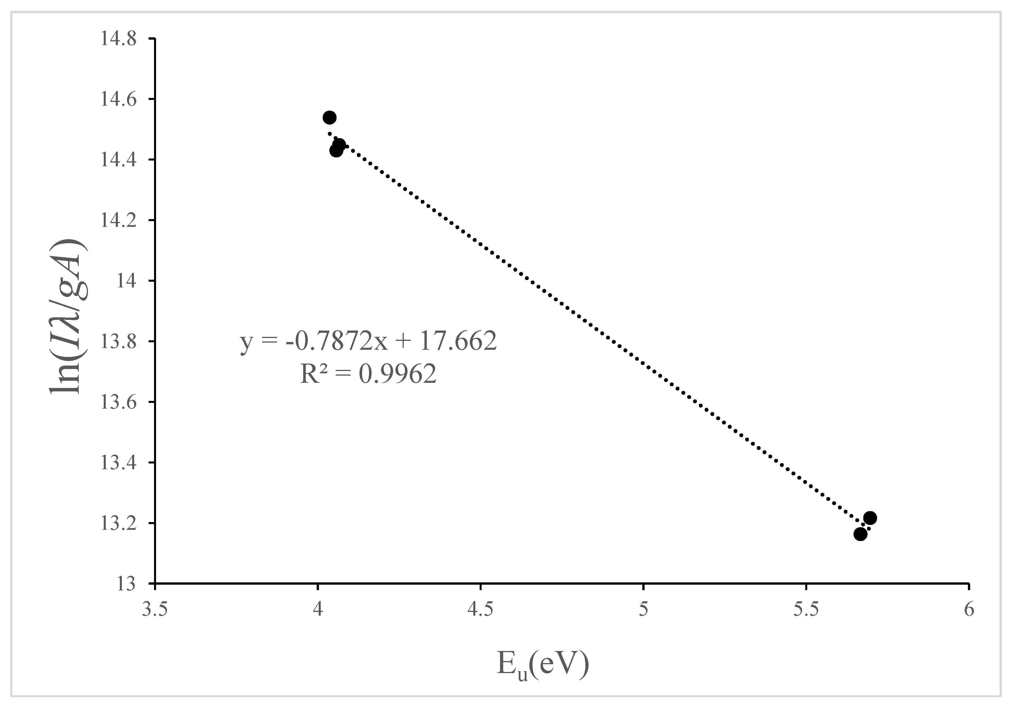
The Boltzmann plots for the Martian data produced correlation coefficients (R
2) primarily above 0.80; a sample plot is shown in
Figure 1.
Table 1 shows the temperatures calculated for the Martian samples. The average temperature was found to be 18,900 K. Please note only a small subset of the data is shown here; the average, standard deviation, and %RSD (relative standard deviation) shown in the table is representative of all the temperatures calculated, which were 1184 temperatures in total. It is not known how the names of each site analyzed were determined; this information could not be found. It is known that the rover traveled and took its LIBS data within a 12 mile stretch of the Gale crater on Mars for the data used in this study. The Martian temperature data showed higher variation in the calculated plasma temperatures. This larger variation in plasma temperatures could be attributed to many different factors. Since the atmospheric pressure and composition are mostly consistent across Mars, and the Curiosity rover stayed within the Gale crater and did not travel a large distance between locations, it is unlikely that these factors caused the variations. Instead, it was likely other factors such as incident laser intensity, spot size and even the distance from the target surface were responsible for these variations in plasma temperatures [
6]. In fact, given the large range of distances over which the LIBS system was used—up to 14 m [
3]—it is possible that the variations in temperature and spectral intensity were caused by these different distances.
It should be noted that about 280 LIBS Martian spectra could not be used for plasma temperature determination. This was due to the fact that these spectra did not contain any atomic lines or there were no titanium lines found in the region of interest. The actual cause of the unusable spectra could be attributed to multiple issues like the detector on the ChemCam not picking up any light or being too far away. According to NASA, the ChemCam device was effective at a range of 14 m [
1,
2,
3].
The Boltzmann plots on the Earth samples showed correlations of generally above 0.78. The average temperature was found to be 15,900 K in the 1 μs time delay data. Also, there was not as much variation in temperature as in the Martian data; these data are shown in
Table 2. This lower variation in the Earth data is most likely due to the fact that the LIBS system parameters of laser energy, lens-to-sample distance, and placement of collection fiber were constant for this part of the experiment and/or there was a smaller data set.
Figure 2 shows a comparison between the average temperatures calculated from the Martian and Earth samples. The graph clearly shows that the temperatures calculated from the Earth samples were generally lower than the Martian samples. It also shows that the average temperatures were not significantly different from each other. It was thought that the potential cause for the lower plasma temperatures on Earth could be due to the fact that the data were taken in gated mode and the earliest part of the plasma formation where the plasma is hottest was not taken in account. However, these data were also taken using a zero-microsecond time delay with a 20 μs gate width; analysis of these data shows a slightly lower plasma temperature than the one-microsecond time delay; these data were added in
Table 2. The temperatures were lower using a time delay of 0 μs but they were not significantly different from the 1 μs time delay temperature data. The average temperature here was determined to be 13,200 K.
For the electron density determination of the Martian samples, the data files that produced no temperature results were neglected for this analysis. There were only about 80 samples that contained no carbon interference with the hydrogen line or for which the carbon peak did not interfere with the FWHM calculation. For the rest of the data, there was a large carbon line which interfered with the hydrogen line such that the FWHM could not be determined easily (
Figure 3); this is due to the atmosphere of Mars, which is approximately 95% CO
2. For some of this data, it was possible to predict the other half of hydrogen peak to allow for calculation of its FWHM by using a computer program written. This allowed for electron density calculations for about 270 more samples. The electron density results showed slightly less variation than the temperature results; this is most likely due to the smaller subset of usable data. A smaller subset of the electron density data from the Martian data is shown in
Table 3; the average electron density in these data was determined to be 2.17 × 10
17 cm
−3. For the Earth samples, there was no carbon interference with the hydrogen line; therefore, the FWHM and electron densities were easy to determine. The electron density results for the Earth samples are shown in
Table 2.
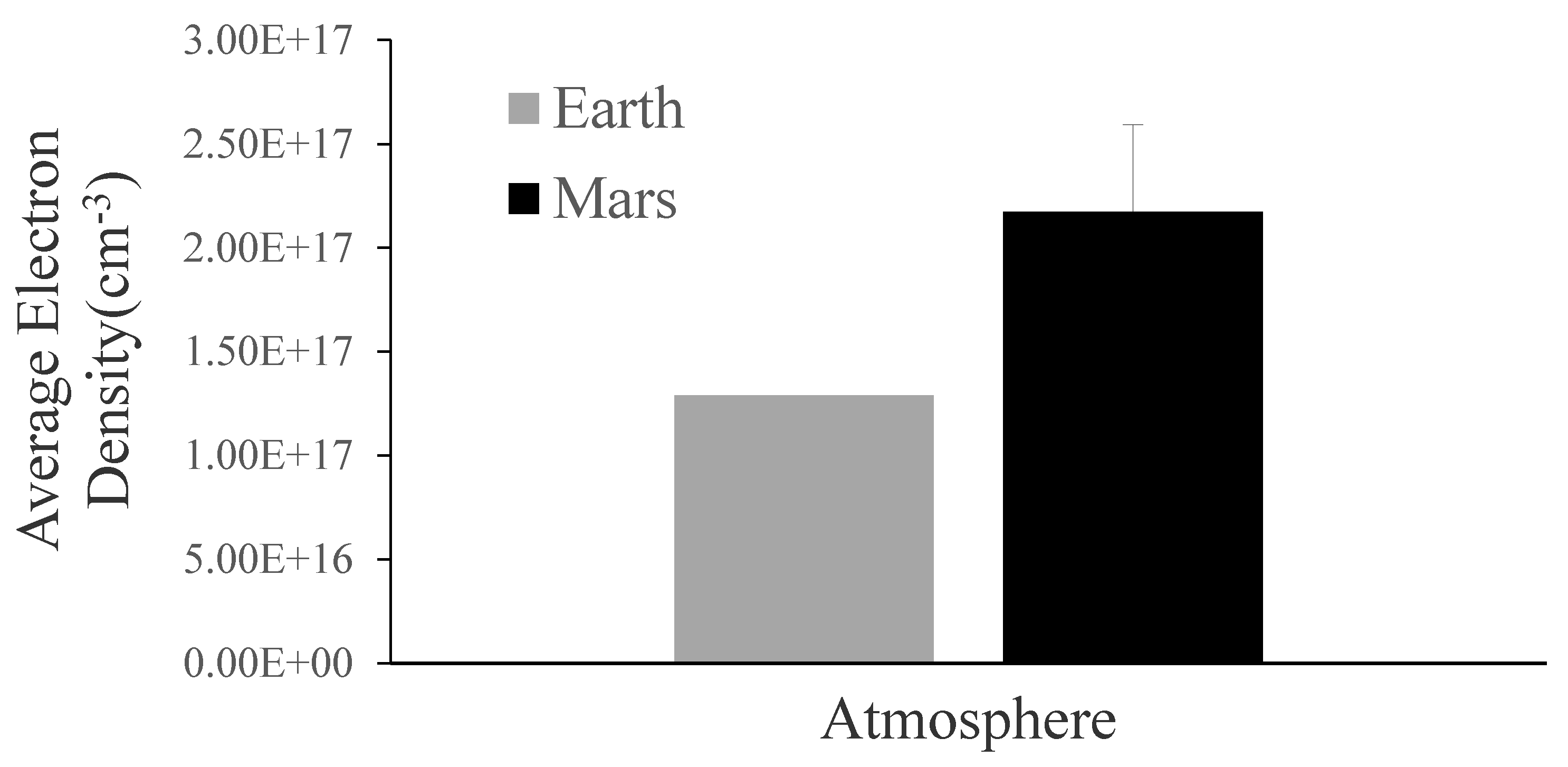
Figure 4 shows a comparison between the average electron densities of the Martian and Earth samples. It is clearly shown that the Earth samples have a significantly lower electron density than the Martian samples. A prior study reported an electron density range of 1.5 to 2.0 × 10
17 cm
−3 for a synthetic silicate sample using a time delay of 0.5 μs with a 4.5 μs gate width over energies ranging from 10 mJ to 100 mJ under normal atmospheric conditions on Earth [
13]. This current study reports an average of 1.29 × 10
17 cm
−3; this is close to the lower energy values from the previous study and the small difference is most likely due to the time delay and gate width differences. The Martian data showed a larger average electron density using similar energy parameters; it is less than a twofold increase but the results show that the electron densities from the Martian and Earth data are significantly different from each other and that there is more broadening in the hydrogen line with the Martian data.
The electron density data were also worked up using the Si (I) line at 250.69 nm due to some discrepancies as noted in the discussion below. All 1184 Martian files were able to be used for electron density determination in this data set.
Table 2 and
Table 3 contain the electron density using the silicon line for the Earth data and Martian data, respectively. These data show a significant decrease in electron density with the Martian data; however, it is less than a twofold decrease. This is further discussed below.
3. Discussion
The results in electron density using the hydrogen line from the Martian data tend to contradict what other studies have predicted about the electron density of plasma under Martian conditions. Some research suggests and shows that higher pressures cool the sample the more quickly and increase the Stark broadening, thus increasing the overall electron density. Plasmas formed in lower pressures have a reduction in cooling which decreases the Stark broadening and electron density and allows for increased resolution; this is why the Martian conditions tend to have increased resolution [
14,
15,
16,
17,
18,
19,
20,
21]. The calculated electron densities in Earth’s atmosphere reported here are corroborated with prior results using the same hydrogen line [
13]. Electron density higher by a factor of two is predicted by Griem’s theory using this hydrogen line [
22], but, since the same line and calculation was used for both sets of data (Earth’s and Mars’s), this impact is not considered here. The Salle paper suggests that lower pressures cause less stark broadening for elements that are found at higher concentrations which have lower energy upper levels that end near the ground state [
17]. Their paper also shows that there was no effect on Stark broadening for lower concentration elements with the same types of transitions previously mentioned and for elements at higher concentrations with higher energy upper levels that end in higher energy lower levels [
17]. The hydrogen line used here has a higher energy upper level (12.1 eV) and ends in a higher energy lower level (10.2 eV). Both atmospheres (Earth’s and Mars’s) have trace amounts of hydrogen present. This potentially means that there are other effects, which are causing the increased Stark broadening of the hydrogen line on Mars. A possible explanation for this line broadening increase could be due to elemental concentration effects. There are some studies that suggest that elements found at higher concentrations can produce more ion–electron recombination in the plasma which reduces the overall spectral intensities and causes a wider line profiles leading to increased electron densities [
23,
24]. A reduction in the emission intensities is shown in the Salle and Colao papers for the spectral data under a simulated Martian atmosphere. Even though better signal-to-background ratios are calculated for the detected lines in simulated Martian conditions, the overall spectral intensities were decreased under Martian conditions [
17,
21]. The Colao paper does show reduced electron densities in the CO
2 atmosphere due to a narrowing of the neutral silicon line in their spectral data; their electron density was calculated using the neutral silicon line at 250.69 nm. Their samples chosen contained a larger amount of silicon and this silicon line used in their electron density calculation has a lower energy upper level and ends near the ground state; as reported in the Salle paper, the use of this silicon line may be why they saw reduced electron densities under simulated Martian conditions [
17,
21]. A confirmation of this effect was done by measuring the FWHM of the Si I at 250.69 nm and calculating in all of the Martian data where the plasma temperatures were calculated (1184 files total) and the Earth data. The FWHM of the Si I line in the Earth data was larger than the FWHM of the Si I line in the Martian data. The average electron density using the Si I emission line was determined to be 1.46 × 10
18 cm
−3 with a 7.79% RSD and 1.04 × 10
18 cm
−3 with a 24% RSD for the Earth and Mars data, respectively. Both the Earth and Mars data produced much higher electron densities using the silicon line; this was by a factor of approximately 11 and 5 in the Earth and Mars data, respectively. A further examination of different line broadening methods could be explored to help improve the accuracy within the data. Comparing the electron density calculated with the silicon line for the Earth and Mars data, it is clearly shown that the Mars data produced a lower electron density than the Earth data; this shows the pressure, transition, and concentration dependence of the Si I line as noted in the Salle paper [
17] while the calculated electron density using the H line does not have this pressure, transition, and concentration dependence and shows an increase in the electron density with the Martian data.
Furthermore, it should be noted that there are many other LIBS variables other than sample composition and atmosphere which can affect the obtained LIBS spectrum; some of these include laser wavelength, timing parameters, pulse energy, number of laser shots, and the angle of incidence between the laser pulse and sample. This study had no control over the parameters such as target distance, spot size or light collection for the Martian samples, since the rover was controlled by NASA. Even though the samples taken on Earth were made to match some of the rover parameters such as laser energy, other factors such as the varying distance to the target of some samples, could likely affect the Martian data and lead to some variation in the plasma temperature and electron density on those samples [
1,
3,
8,
9]. Certain trends, especially the presence of a large carbon line and the generally higher plasma temperatures are likely a result of the combined Martian atmosphere and sample composition. Discrepancies in electron density results need a further examination. This could be done by simulating a Martian atmosphere on Earth for a more detailed study to examine this effect.
4. Material and Methods
Sample Preparation: The Earth-based samples were synthetic silicate (GBW 07709), red soil (VS 2501–83), black soil (VS 2507–83), and soil (NCS DC73029); these were purchased from Brammer Standards, Houston, TX. These samples were pressed into 35 mm pellets using a hydraulic press (Carver, Model-C, Wabash, Indiana) to create a smooth surface for LIBS analysis.
LIBS Instrumentation: The Martian data were collected by NASA ChemCam equipment on the Curiosity rover. A description of the ChemCam system is published elsewhere; this contains a brief overview of the system [
1,
2,
3]. The ChemCam used a Nd:KGW laser that produced 5 ns pulses at 1067 nm with energies of up to 14 mJ reaching the sample. No gate delay was used for the Martian samples as it was unnecessary in Martian conditions. The ChemCam system on the MSL is split into a mast unit and a body unit. The mast unit contains the laser, a telescope, and a remote microimager. The telescope is used to collect the plasma light created by the laser and transmit it into a fiber optic cable that sends the light to three spectrometers. The light is then detected using CCDs (charged coupled devices). The telescope allows the LIBS system to analyze samples up to 7 m away with 10% accuracy. The body unit housed the three spectrometers. The spectrometers operated in a range from 242–800 nm, excluding 335–385 nm, and 465–510 nm. The spectrometers had a resolution of 0.2 nm. The detectors on these spectrometers were a two-dimensional CCD array. The laser, spectrometer, and CCDs were all synchronized with the laser. The body unit also contained a system for onboard calibration. The ChemCam calibration target assembly (CCCT) contained at least one sample to similar to each of the expected rock types. Each target could accommodate 100 analyses of 75 laser pulses [
1,
2,
3]. The LIBS Rover took data for each laser shot for each site at each location on that site. The data used here analyzed an accumulation of shot numbers 7 through 16 for location 1 of each site analyzed; shots 1–6 were excluded because those shots were considered to allow the laser to remove the sample area of possible contamination. This data set used here contained over 14,000 data files. There were a total of 1454 sites and ten shots were accumulated for each site. Therefore, 1454 LIBS spectra were analyzed for this part of the project. The data are open access [
12], but the data used for this study were downloaded via another website where the files were reformatted to make them easier to use [
25].
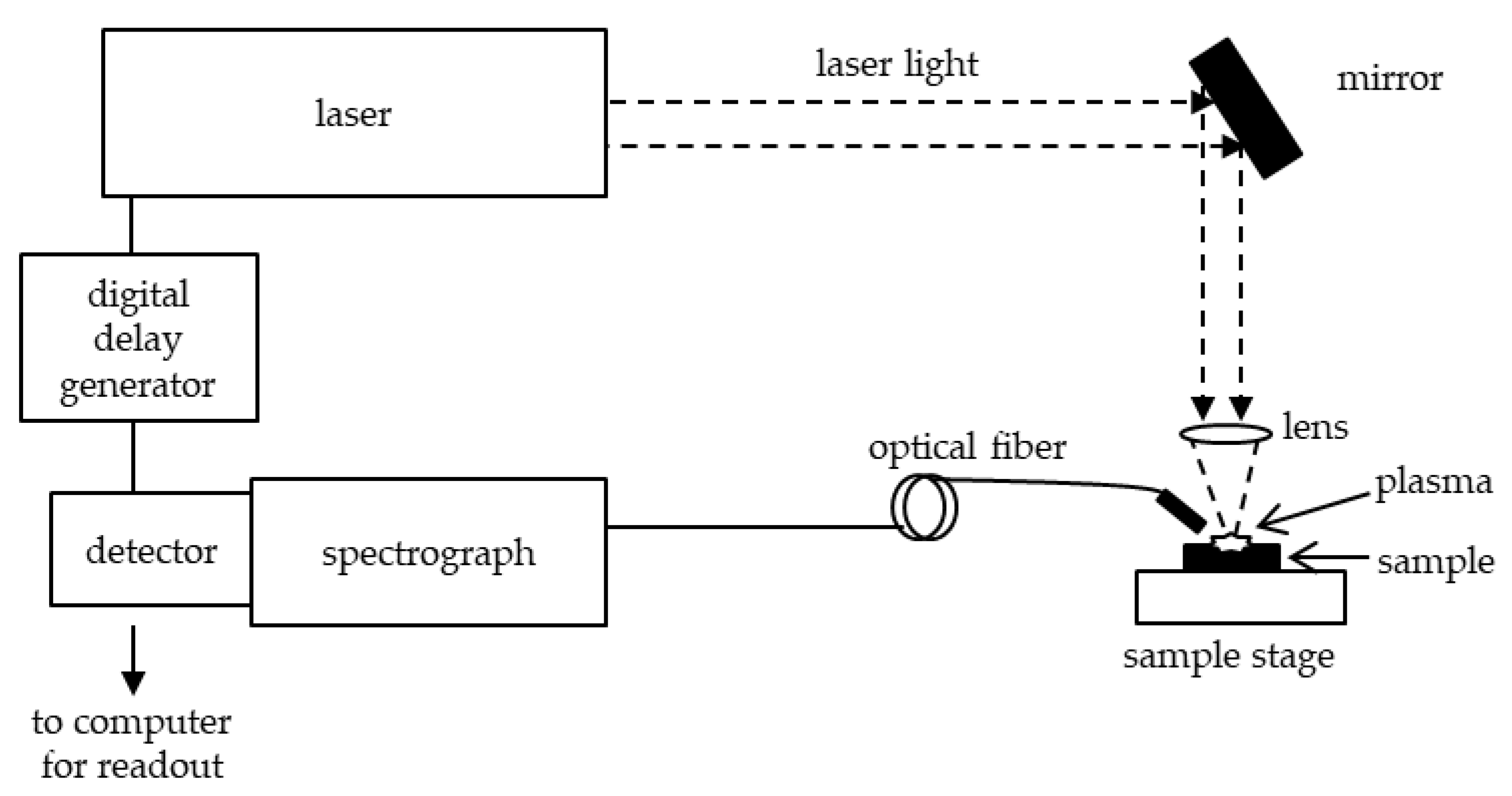
The Earth data were taken with a laboratory LIBS set-up using a Nd: YAG laser (Surelite II, Continuum, Santa Clara, CA, USA) operating at 1064 nm using a laser energy of 12 mJ. A 75 mm focal length lens was used to focus the laser pulse onto the sample. The light was collected by an optical fiber (QP1000–2-UV-VIS, Ocean Optics, Dunedin, FL, USA) placed near the sample. The light was spectrally resolved and detected with an echelle spectrograph (SE200, Catalina, Tucson, AZ, USA) with an ICCD (DH-734–18F-03 IStar, Andor Technology, Belfast, Ireland). The approximate resolving power of the echelle/ICCD is approximately 1700. The laser was operated at 10 Hz. A time delay of 1 µs and a 20 µs gate width were used with a gain of 125 and a three-second exposure; each sample spot represents an accumulation of 30 laser shots. The timing between the laser and detector, the gate-delay, was controlled using a digital delay generator (BNC Model 575–4C Digital Delay and Pulse Generator, Berkeley Nucleonic Corp., San Rafael, CA, USA). Each sample was analyzed five times. The Earth-based LIBS setup is shown in
Figure 5.
Boltzmann plot method: To determine the plasma temperature using the Boltzmann plot method, Equation (1) is used; this gives the spectral line gradient intensity [
4,
7].
In Equation (1),
I is the intensity of the transition,
h is Planck’s constant,
v is the frequency,
g is the degeneracy,
A is the transition probability,
N is the absolute number or number density,
c is the speed of light,
N0 is the total species population,
λ is the wavelength,
Z is the partition function,
Eu is the energy of the upper state of emission,
k is the Boltzmann constant, and
T is the temperature [
8].
Rearranging Equation (1) to a linear line format allows for graphical analysis as seen in equation
To create the Boltzmann plot, ln(
Iλ/
gA) is plotted against
Eu in eV. Equation (2) takes the general form of a line, y = mx + b where x is the
Eu, y is the ln(
Iλ/
gA), and the slope, m, is −1/
kT. The
Eu,
A, and
g can be found using the National Institute of Standards and Technology (NIST) database; the intensity and wavelength data can be found from the spectra [
26].
The Boltzmann plots (
Figure 1) were created for the Mars and Earth spectra using a set of titanium lines between 300 and 310 nm. A linear trendline was applied to each of the plots. The temperatures were calculated using the slope of the linear fit [
8]. These temperatures were then used to help calculate the electron density of the samples, as explained below. All of the data work up was done in Microsoft Excel.
Electron density method: For calculating the electron densities, the method of using full width at half-maximum (FWHM) with the Stark broadening of spectral lines was used. To determine the electron density of a sample, the FWHM of the hydrogen line at 656.3 nm line was used; this corresponds to a Balmer alpha line for hydrogen. The linear Stark width for hydrogen lines is shown in Equation (3).
where N
e is the electron density,
λ1/2 is the FWHM, and α
1/2 is reduced wavelength, which is dependent on both electron density and temperature of the plasma. The values for α
1/2 are provided in Griem’s 1974 Appendix IIIa [
4,
8,
9].
The FWHM of the hydrogen was determined for all samples. A Microsoft Excel file was created to calculate the electron density at various temperatures. The FWHM was used to calculate the electron density using the created Excel spreadsheet [
8].
On most of the Martian data, a carbon line (658.8 nm) caused some interferences with the 656.3 nm hydrogen line; this is shown in
Figure 3. Since the peaks tend to be symmetrical in nature, a computer program was created to trace the other portion of the hydrogen and calculate the FWHM of those affected Martian files. The program algorithm was written as follows:
- (1)
Input the specific wavelength range containing the pertinent peaks;
- (2)
Find the wavelength corresponding to the carbon peak;
- (3)
Find the position of the hydrogen peak, which was lower than the carbon peak;
- (4)
Determine the baseline that is the position corresponding to the minimum density at the left of the carbon peak;
- (5)
Determine the half-height;
- (6)
Trace the missing portion of the hydrogen peak using the symmetric method;
- (7)
Find the position on the electron density curve when the y value of the position is equal to half-height;
- (8)
Calculate the FWHM.
The program in this paper was run in the Microsoft Windows 10 64 bit operating system. The computer was configured with a 16-GB Intel (R) Core (TM) i7–7700 processor. The computer program was implemented in Matlab (R2018a, The Mathworks Inc., Natick, MA, USA).
The Stark width calculation for the Si line at 250.69 nm is shown in Equation (4):
where
Δλ1/2 is the FWHM,
w is the electron impact half-width,
Ne is the electron density, A is the ion-broadening parameter, and
ND is the number of particles in the Debye sphere. This equation can be simplified to Equation (5) due to the minimal effect of the second term [
27]. Equation (5) was used to calculate the electron density for the Mars and Earth data.
The electron impact half-width for the Mars and Earth data was calculated by plotting the
w’s vs. temperature provided by Griem’s
Plasma Spectroscopy [
28] and interpolating the
w for the Mars and Earth data based on the calculated temperatures for each spectral file.
A computer program was written to calculate the FWHM of all of the Martian data where temperature results were obtained; this included 1184 files. The program was written (1) to find the position of highest intensity of the silicon peak, (2) to find the position of the minimum intensity in the set wavelength range to determine the baseline, (3) to find the position of the half height between the baseline and silicon peak and (4) to calculate the FWHM distance. The same computer and program were used as noted above for the hydrogen line.


