Radiative Cascade Repopulation of 1s2s2p ⁴P States Formed by Single Electron Capture in 2–18 MeV Collisions of C⁴⁺ (1s2s ³S) with He

Abstract

This study focuses on the details of cascade repopulation of doubly excited triply open-shell C${}^{3+}\left(1s2s2p\right)$ ${}^{4}P$ and ${}^2{P}_{\pm }$ states produced in 2–18 MeV collisions of C${}^{4+}\left(1s2s{}^{3}S\right)$ with He. Such cascade calculations are necessary for the correct determination of the ratio R of their cross sections, used as a measure of spin statistics [Madesis et al. PRL 124 (2020) 113401]. Here, we present the details of our cascade calculations within a new matrix formulation based on the well-known diagrammatic cascade approach [Curtis, Am. J. Phys. 36 (1968) 1123], extended to also include Auger depopulation. The initial populations of the $1s2sn\ell {}^{4}L$ and $1s2sn\ell {}^{2}L$ levels included in our analysis are obtained from the direct $n\ell$ single electron capture (SEC) cross sections, calculated using the novel three-electron close-coupling (3eAOCC) approach. All relevant radiative branching ratios (RBR) for $n\le 4$ were computed using the COWAN code. While doublet RBRs are found to be very small, quartet RBRs are found to be large, indicating cascade feeding to be important only for quartets, consistent with previous findings. Calculations including up to third order cascades, extended to $n\to \infty$ using an $n^{-3}$ SEC model, showed a ∼60% increase of the $1s2s2p{}^{4}P$ populations due to cascades, resulting, for the first time, in R values in good overall agreement with experiment.

1. Introduction

Highly excited (autoionizing) atomic and ionic states can be produced in ion-atom and ion-electron collisions by various processes such as inner-shell excitation, ionization, electron capture (to excited states), and/or their combinations. These states then relax to lower energy states and the ground state via radiative and/or Auger decays in a stepwise manner, known as cascades, resulting in the repopulation of the intermediate levels. Cascade repopulation of intermediate levels is also common to atoms and multi-charged ions in laboratory plasmas [1,2], as well as astrophysical plasmas encountered in solar coronas, gas nebulae and active galactic nuclei (AGN) [1,3,4]. The complex character of the stepwise cascade process, an inherent, but usually unwanted side effect in most investigations, has received considerable attention, studied primarily by simulations [5,6,7,8]. Such studies have focused on mostly radiative cascades related to recombination in He-like ions [9], emission of polarized X-rays [10], X-ray fusion diagnostics [11], shake-off effects [12], solar wind [13] and electron capture in H-like ions [14,15,16], just to mention a few. Cascade repopulation affects the accurate determination of cross sections, therefore adding uncertainty in the comparison with theory, which eventually must also include the additional cascade contributions by performing a detailed cascade feeding analysis. Moreover, cascades have been an ever present limitation in the precise determination of lifetimes [17] using beam-foil spectroscopy [18,19,20,21,22].

Some of the most investigated states in ion-atom collisions are the Li-like doubly excited quartet $1s2snl{}^{4}L$ states. In particular, the lowest-lying $1s2s2p{}^{4}P$ state, which is also metastable, has been under study since the early 70s, first observed in the ions of Be${}^{+}$, B${}^{2+}$ and F${}^{6+}$ [23], C${}^{3+}$ [24], O${}^{5+}$ and F${}^{6+}$ [25,26], Li [27], as well as in highly charged heavier ions such as Cl${}^{14+}$ and Ar${}^{15+}$ [28]. For a general review of optical studies of these states, see also [29] and references therein.

Of more recent interest has been the ratio R of $1s2s2p$ ${}^{4}P{/}^{2}P$ cross sections [30]. In the case of $2p$ single electron capture (SEC) in collisions of $1s2s{}^{3}S$ ions with He and H${}_2$, R has been considered to be an indicator of spin statistics [31,32,33,34,35]. Indeed, this ratio results in $R=1$, when considering only spin multiplicity, while $R=2$ in the frozen core approximation, where only the ${}^{4}P$ and a single ${}^{2}P$ state can be produced from the $1s2s{}^{3}S$ initial state [34,36,37]. Such statistical arguments and approximations are often used to simplify difficult problems of computing relative populations in high energy plasmas [4] and can therefore be of important practical use. Very recently, we reported [30] that in collisions using C${}^{4+}\left(1s2s{}^{3}S\right)$ projectile ions, a complete breakdown of the frozen core treatment used for SEC to date is observed, as regards to spin statistics in this highly correlated dynamical atomic system. Furthermore, we showed that only a new dynamical calculation involving three active electrons is found to give results consistent with experiment, with radiative cascade repopulation playing an important role.

Here, we present the details of modeling this radiative cascade feeding of the doubly excited C${}^{3+}$ $1s2s2p{}^{4}P$ and $1s2s2p{}^{2}P$ levels formed by SEC. Our cascade calculation is based on a new, elegant, and easy to use matrix formulation extending the well-known diagrammatic approach of Curtis [38]. The necessary radiative and Auger transition rates were computed using the COWAN [39] atomic structure code, while the initial state populations were taken from our recent publication [30], where they were computed using the new three-electron atomic orbital close-coupling (3eAOCC) approach.

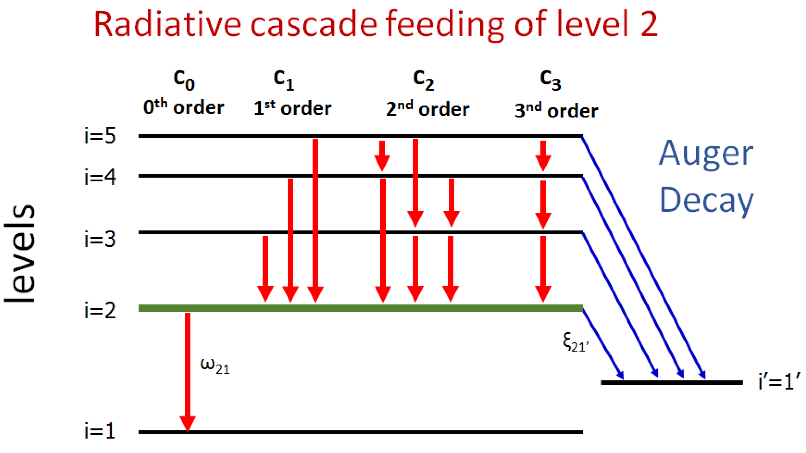
2. Mathematical Description of Radiative Cascade Feeding

In this section, we present our mathematical description of radiative cascades extending the treatment of Curtis [38] to also include Auger depopulation. These Auger transitions are important in the case of the C${}^{3+}\left(1s2s2p{}^{4,2}P\right)$ states [35], to which we apply our otherwise general treatment. An elegant, cascade matrix formulation is used making the cascade calculations much easier to evaluate to any desired cascade order, as required.

2.1. Definitions—The Cascade Rate Equation

We consider a set of m levels labeled consecutively in order of decreasing binding energies $E_i$ from 1 to m. The population at time t of the j-th level denoted $N_j\left(t\right)$ with energy $E_j$ is assumed to be the result of cascade feeding from higher energy levels ($k>j$) by radiative transitions with rates $A_{kj}^r$ and photon energies $\hslash {\omega }_{kj}=E_k-E_j$, as well as depopulation by radiative transitions to all lower energy levels $f=1,2,\dots ,j-1$, with rates $A_{jf}^r$. Additional depopulation can also occur due to autoionizing (including Auger and Coster-Kronig) transitions, which remove population from the level j to all final states $f^{\prime }$, with the rate $A_{j{f}^{\prime }}^a$. The final states $f^{\prime }$ of the autoionizing transitions correspond to a different set of electronic configurations from those of the radiative transitions (the ion charge is reduced by one in the case of autoionization) and are therefore denoted by a prime. An example of the schematic decay of a 5-level system ($m=5$) is shown in Figure 1.

The coupled differential equations governing the population of any particular level $n\in [1,m]$ (i.e., the general index j now has the specific value $j=n$) are then readily given [38] with the addition of the depopulating autoionization channel [35]1 by:

$$\begin{array}{cc}\hfill \frac{d{N}_n}{dt}& =\sum _{i=n+1}^m{A}_{in}^r{N}_i\left(t\right)-\left(\sum _{f=1}^{n-1}{A}_{nf}^r+\sum _{f^{\prime }}{A}_{n{f}^{\prime }}^a\right)N_n\left(t\right)=\sum _{i=n+1}^m{A}_{in}^r{N}_i\left(t\right)-{\alpha }_n{N}_n\left(t\right),\hfill \end{array}$$

(1)

with ${\alpha }_n$ defined as2:

$$\begin{array}{cc}\hfill {\alpha }_n& \equiv \sum _{f=1}^{n-1}{A}_{nf}^r+\sum _{f^{\prime }}{A}_{n{f}^{\prime }}^a=\frac{1}{{\tau }_n}.\hfill \end{array}$$

(2)

Thus, ${\alpha }_n$ is seen to be the total decay rate ($=\hslash {\mathsf{\Gamma }}_n$, where ${\mathsf{\Gamma }}_n$ is the total width) of level n, i.e., the inverse of its lifetime ${\tau }_n$, and is defined as the sum of all transition probabilities between level n and all lower-lying levels, including Auger decays. In ${\alpha }_n$ (Equation (2)), we now include both radiative and Auger decays, thus extending the treatment of Curtis [38] (which only included the radiative term $A_{nf}^r$ in ${\alpha }_n$). This is seen not to change the overall mathematical form of the rate equation which remains:

$$\begin{array}{cc}\hfill \frac{d{N}_n}{dt}+{\alpha }_n{N}_n\left(t\right)& =\sum _{i=n+1}^m{A}_{in}^r{N}_i\left(t\right).\hfill \end{array}$$

(3)

It is helpful to also introduce the notions of the partial fluorescence yield ${\omega }_{nf}$ and the partial Auger yield ${\xi }_{n{f}^{\prime }}$, in addition to the fluorescence yield ${\omega }_n$ and the Auger yield ${\xi }_n$ [42]:

$$\begin{array}{cc}\hfill {\omega }_{nf}& =\frac{A_{nf}^r}{{\alpha }_n}\mathrm{and}{\omega }_n=\frac{A_n^r}{{\alpha }_n},\hfill \end{array}$$

(4)

$$\begin{array}{cc}\hfill {\xi }_{n{f}^{\prime }}& =\frac{A_{n{f}^{\prime }}^a}{{\alpha }_n}\mathrm{and}{\xi }_n=\frac{A_n^a}{{\alpha }_n},\hfill \end{array}$$

(5)

where we have also introduced the total radiative $A_n^r$ and total Auger $A_n^a$ rates for level n:

$$\begin{array}{c}\hfill A_n^r\equiv \sum _{f=1}^{n-1}{A}_{nf}^r\mathrm{and}{A}_n^a\equiv \sum _{f^{\prime }}{A}_{n{f}^{\prime }}^a,\end{array}$$

(6)

and therefore we also have:

$$\begin{array}{c}\hfill {\alpha }_n=A_n^r+A_n^a\mathrm{and}{\omega }_n+{\xi }_n=1.\end{array}$$

(7)

Thus, ${\omega }_{nf}$ and ${\xi }_{n{f}^{\prime }}$, are equivalent to probabilities for the state n to decay either radiatively or by autoionization to any one of the final states f or $f^{\prime }$, respectively. The partial fluorescence yield ${\omega }_{ij}$ is also known as the radiative branching ratio (RBR).

Equation (3) can be readily solved by multiplying both sides by the integrating factor $exp\left({\alpha }_{n}t\right)$ and performing the integration after exchanging the order of sum and integral [38] to give an iterative solution that can be readily programmed to give analytic results:

$$\begin{array}{cc}\hfill N_n\left(t\right)& =\left[N_n\left(0\right)+\sum _{i=n+1}^m{A}_{in}^r{\int }_0^{t}d{t}^{\prime }exp\left({\alpha }_n{t}^{\prime }\right)N_i\left(t^{\prime }\right)\right]exp(-{\alpha }_{n}t).\hfill \end{array}$$

(8)

Inclusion of the depopulating Auger transitions in the definition of ${\alpha }_n$ (Equation (2)) does not change the form of the differential equation (Equation (3)), thus having exactly the same solution as Equation (8), like the ones given by Curtis [38]. However, the result is more general and, as seen in the case of the $C^{3+}(1s2s2p{}^{4,2}P$) level populations, plays an important role in the detailed understanding of the cascade feeding mechanism, which is found to selectively enhance the population of the quartets compared to that of the doublets [30,33,35].

2.2. Time-Dependence of Level Populations and Cascade Feeding Orders

The first three iterations of Equation (8) can be readily computed after performing the trivial integrations. Defining the radiative cascade feeding orders $c_0,c_1,c_2$, we have [38]:

$$c_0:N_n^{c_0}\left(t\right)=N_n\left(0\right)exp(-{\alpha }_{n}t),$$

(9)

$$\begin{array}{cc}{c}_1:N_n^{c_1}\left(t\right)\hfill & =\left[\sum _{i=n+1}^m{N}_i\left(0\right)A_{in}^r{\int }_0^{t}d{t}^{\prime }exp\left[({\alpha }_n-{\alpha }_i)t^{\prime }\right]\right]exp(-{\alpha }_{n}t)\hfill \\ \hfill & =\sum _{i=n+1}^m{N}_i\left(0\right)A_{in}^r\left[\frac{exp(-{\alpha }_{i}t)}{({\alpha }_n-{\alpha }_i)}+\frac{exp(-{\alpha }_{n}t)}{({\alpha }_i-{\alpha }_n)}\right],\hfill \end{array}$$

(10)

$$\begin{array}{cc}\hfill c_2:N_n^{c_2}\left(t\right)& =\left[\sum _{i=n+1}^{m-1}\sum _{j=i+1}^m{N}_j\left(0\right)A_{ji}^r{A}_{in}^r{\int }_0^{t}d{t}^{\prime }exp\left[({\alpha }_n-{\alpha }_i)t^{\prime }\right]{\int }_0^{t^{\prime }}d{t}^{\prime \prime }exp\left[({\alpha }_i-{\alpha }_j)t^{\prime \prime }\right]\right]exp(-{\alpha }_{n}t)\hfill \\ \hfill & =\sum _{i=n+1}^{m-1}\sum _{j=i+1}^m{N}_j\left(0\right)A_{ji}^r{A}_{in}^r\left[\frac{exp(-{\alpha }_{j}t)}{({\alpha }_i-{\alpha }_j)({\alpha }_n-{\alpha }_j)}+\frac{exp(-{\alpha }_{i}t)}{({\alpha }_j-{\alpha }_i)({\alpha }_n-{\alpha }_i)}+\frac{exp(-{\alpha }_{n}t)}{({\alpha }_j-{\alpha }_n)({\alpha }_i-{\alpha }_n)}\right],\hfill \end{array}$$

(11)

with the total contribution up to and including cascade order $c_k$, $N_n\left(t\right)[\le c_k]$, readily computed using Equation (8) and given by the sum:

$$\begin{array}{cc}\hfill N_n\left(t\right)[\le c_k]& =N_n^{c_0}\left(t\right)+N_n^{c_1}\left(t\right)+N_n^{c_2}\left(t\right)+\dots +N_n^{c_k}\left(t\right)=\sum _{i=0}^k{N}_n^{c_i}\left(t\right).\hfill \end{array}$$

(12)

We note that the $t=0$ initial level populations $N_i\left(0\right)$ above, refer to the i-th level populations before cascading begins and are independently calculated, as discussed in detail in Section 3.3.

Referring to Figure 1, the 0-th order cascade term $c_0$ corresponds to the depopulating of level n of interest, either by an Auger or a radiative transition, to all available levels below it, while cascade orders $c_k$ (with $k\ge 1$) correspond to the populating of level n from all higher-lying energy levels. The initial population of level n at time $t=0$, i.e., in the absence of cascade feeding, is usually the primary process under investigation. Here, this is the direct $2p$ SEC leading to the production of the $1s2s2p$ ${}^{4}P$ and ${}^{2}P$ states detected by their Auger decay [30,43]. The higher order cascades usually constitute an unwanted complication that needs to be understood and quantified before accurate cross section information can be extracted about the population of level n due to just the primary process.

The first-order cascade term $c_1$ corresponds to the radiative feeding of the level n from all levels i above it, i.e., $n+1\le i\le m$, by direct one-step radiative $\{i\to n\}$ transitions, i.e., with the emission of 1 photon. The second-order $c_2$ corresponds to the feeding of the level n from all levels j above it, in a two-step radiative transition sequence $\{j\to i\to n\}$, with the first step described by the index j with $i+1\le j\le m$, and the second step by the index i, with the second-step index i within the range $n+1\le i\le m-1$. The second step has its upper limit reduced by 1, i.e., $m-1$, to accommodate the first step which would start in this case from $j=m$, (i.e., $\{j=m\to i\to n\}$). Thus, in the $c_2$ sequence 2 photons are emitted. Similarly, the $c_k$ order results in a sequence of k-steps with the emission of k photons. The contribution of any order k corresponds to the total probability of emitting k sequential photons, each transition contributing with its RBR ${\omega }_{ij}$, and thus is roughly proportional to the product ${\left({\omega }_{ij}\right)}^k$, which therefore rapidly decreases with increasing value of k. The maximum permitted order is clearly determined by the number of levels between n and the highest level $m=M$, where M is the maximum number of levels included in the calculation.

In a typical cascade calculation, it is rare to include contributions beyond the 3rd order ($c_3$), since the convergence of the summation series (Equation (12)) is usually quite rapidly attained. Here, in our calculations (see next sections), we include up to 3rd order cascades, clearly showing that convergence has effectively been attained by $c_2$ for all, but the lowest collision energies3.

2.3. Final Level Populations

Integrating the time-dependent population number $N_n\left(t\right)$ over a sufficiently long detection time ${\tau }_d$, so as to include all the decaying radiative transitions of interest (dipole $E1$ transitions typically occur within the lifetime of any level i, i.e., ${\tau }_i=1/{\alpha }_i$, so we need ${\alpha }_i{\tau }_d>>1$), results in integrals of the type:

$$\begin{array}{c}\hfill {\int }_0^{{\tau }_d}exp(-{\alpha }_{i}t)dt=\frac{1-exp(-{\alpha }_i{\tau }_d)}{{\alpha }_i}\approx \frac{1}{{\alpha }_i}(\mathrm{for}\mathrm{all}{\alpha }_i{\tau }_d>>1),\end{array}$$

(13)

effectively equivalent to integrating over all time, i.e., ${\tau }_d\to \infty$. Thus, integrating over all time, the general expressions for $N_n\left(t\right)$ from Equations (9)–(11) for $c_0$, $c_1$ and $c_2$ cascades we have:

$$c_0:I_n^{c_0}\equiv {\int }_{t=0}^{\infty }dt{N}_n^{c_0}\left(t\right)=\frac{N_n\left(0\right)}{{\alpha }_n},$$

(14)

$$\begin{array}{cc}\hfill c_1:I_n^{c_1}& \equiv {\int }_{t=0}^{\infty }dt{N}_n^{c_1}\left(t\right)=\sum _{i=n+1}^m{N}_i\left(0\right)A_{in}^r\left[\frac{1}{({\alpha }_n-{\alpha }_i){\alpha }_i}+\frac{1}{({\alpha }_i-{\alpha }_n){\alpha }_n}\right]\hfill \\ \hfill & =\sum _{i=n+1}^m\frac{N_i\left(0\right)}{{\alpha }_n}\frac{A_{in}^r}{{\alpha }_i}=\frac{1}{{\alpha }_n}\sum _{i=n+1}^m{N}_i\left(0\right){\omega }_{in},\hfill \end{array}$$

(15)

$$\begin{array}{cc}\hfill c_2:I_n^{c_2}& \equiv {\int }_{t=0}^{\infty }dt{N}_n^{c_2}\left(t\right)\hfill \\ \hfill & =\sum _{i=n+1}^{m-1}\sum _{j=i+1}^m{N}_j\left(0\right)A_{ji}^r{A}_{in}^r\left[\frac{1}{{\alpha }_j({\alpha }_i-{\alpha }_j)({\alpha }_n-{\alpha }_j)}+\frac{1}{{\alpha }_i({\alpha }_j-{\alpha }_i)({\alpha }_n-{\alpha }_i)}+\frac{1}{{\alpha }_n({\alpha }_j-{\alpha }_n)({\alpha }_i-{\alpha }_n)}\right]\hfill \\ \hfill & =\sum _{i=n+1}^{m-1}\sum _{j=i+1}^m\frac{N_j\left(0\right)}{{\alpha }_n}\frac{A_{ji}^r}{{\alpha }_j}\frac{A_{in}^r}{{\alpha }_i}=\frac{1}{{\alpha }_n}\sum _{i=n+1}^{m-1}\sum _{j=i+1}^m{N}_j\left(0\right){\omega }_{ji}{\omega }_{in},\hfill \end{array}$$

(16)

and similarly for $c_3$ and so on with

$$\begin{array}{cc}{c}_3:I_n^{c_3}& \equiv {\int }_{t=0}^{\infty }dt{N}_n^{c_3}\left(t\right)=\frac{1}{{\alpha }_n}\sum _{l=n+1}^{m-2}\sum _{i=l+1}^{m-1}\sum _{j=i+1}^m{N}_j\left(0\right){\omega }_{ji}{\omega }_{il}{\omega }_{ln}.\hfill \end{array}$$

(17)

This can be readily extended to include cascades to any order $c_k$ so that in general we have:

$$\begin{array}{cc}\hfill I_n[\le c_k]& ={\int }_{t=0}^{\infty }dt{N}_n\left(t\right)[\le c_k]=I_n^{c_0}+I_n^{c_1}+I_n^{c_2}+\dots +I_n^{c_k}=\frac{N_n[\le c_k]}{{\alpha }_n}=\sum _{i=0}^k{I}_n^{c_i},\hfill \end{array}$$

with the total population of level n up to and including order $c_k$ given by:

$$\begin{array}{cc}{N}_n[\le c_k]& \equiv N_n^{c_0}+N_n^{c_1}+N_n^{c_2}+N_n^{c_3}+\dots +N_n^{c_k}=\sum _{i=0}^k{N}_n^{c_i}\hfill \\ \hfill & =N_n\left(0\right)+\sum _{i=n+1}^m{N}_i\left(0\right){\omega }_{in}+\sum _{i=n+1}^{m-1}\sum _{j=i+1}^m{N}_j\left(0\right){\omega }_{ji}{\omega }_{in}+\sum _{l=n+1}^{m-2}\sum _{i=l+1}^{m-1}\sum _{j=i+1}^m{N}_j\left(0\right){\omega }_{ji}{\omega }_{il}{\omega }_{ln}+\dots ,\hfill \end{array}$$

(18)

with:

$$\begin{array}{cc}\hfill N_n^{c_k}& \equiv {\alpha }_n{I}_n^{c_k}.\hfill \end{array}$$

(19)

These results are clearly what one would intuitively expect by inspecting Figure 1. Thus, in Equation (18), the 0-th cascade order $c_0$ refers to just the initial occupation number $N_n(t=0)$. The 1st cascade order, $c_1$, requires a single radiative transition to feed the state n from all higher-lying states j with probability ${\omega }_{jn}$ and initial occupation number $N_j\left(0\right)$, readily given by ${\sum }_{j=n+1}^m{N}_j\left(0\right){\omega }_{jn}$. The 2nd cascade order, $c_2$, requires the contributions of all possible two-step radiative transition pathways ending on level n, i.e., all two-step pathways $\{j\to i\to n\}$, with probability ${\omega }_{ji}$ and ${\omega }_{in}$ and starting from all initial states j with occupation number $N_j\left(0\right)$. This is readily given by ${\sum }_{i=n+1}^{m-1}{\sum }_{j=i+1}^m{N}_j\left(0\right){\omega }_{ji}{\omega }_{in}$, and so on. Thus, the general result for any order can be readily written down simply by inspection of the cascade level diagram. The clarity of this diagrammatic approach is nicely presented by Curtis [38] and summarized here.

2.4. X-ray and Auger Electron Emission Rates

Experimental information about the n level population comes mostly from either X-ray or Auger electron measurements. The rate of X-rays (or Auger electrons) emitted in a transition from the level n to level f (or $f^{\prime }$, respectively) is given (in #/s) by [33,45]:

$$\begin{array}{ccc}\hfill {\dot{N}}_{nf}^x\left(t\right)\equiv & \frac{d{N}_{nf}^x}{dt}=N_n\left(t\right)A_{nf}^r\hfill & \hfill (\mathrm{characteristic}\mathrm{x}-\mathrm{rays}),\end{array}$$

(20)

$$\begin{array}{ccc}\hfill {\dot{N}}_{n{f}^{\prime }}^e\left(t\right)\equiv & \frac{d{N}_{n{f}^{\prime }}^e}{dt}=N_n\left(t\right)A_{n{f}^{\prime }}^a\hfill & \hfill (\mathrm{Auger}\mathrm{electrons}).\end{array}$$

(21)

Noting from Equation (4) that ${\omega }_{nf}=\frac{A_{nf}^r}{{\alpha }_n}$ and from Equation (5) that ${\xi }_{n{f}^{\prime }}=\frac{A_{n{f}^{\prime }}^a}{{\alpha }_n}$, the total number of X-rays or Auger electrons emitted up to and including order $c_k$ is then given by:

$$\begin{array}{ccc}\hfill N_{nf}^x[\le c_k]=& {\int }_{t=0}^{\infty }dt{\dot{N}}_{nf}^x\left(t\right)=A_{nf}^r{I}_n[\le c_k]={\omega }_{nf}{N}_n[\le c_k]\hfill & \hfill (\mathrm{characteristic}\mathrm{x}-\mathrm{rays}),\end{array}$$

(22)

$$\begin{array}{ccc}\hfill N_{n{f}^{\prime }}^e[\le c_k]=& {\int }_{t=0}^{\infty }dt{\dot{N}}_{n{f}^{\prime }}^e\left(t\right)=A_{n{f}^{\prime }}^a{I}_n[\le c_k]={\xi }_{n{f}^{\prime }}{N}_n[\le c_k]\hfill & \hfill (\mathrm{Auger}\mathrm{electrons}),\end{array}$$

(23)

with $N_n[\le c_k]$ given by Equation (18).

Here, we have used the technique of zero-degree Auger projectile spectroscopy (ZAPS) [46] to obtain the level populations of the $1s2s2p$ ${}^{4}P$ and ${}^2{P}_{\pm }$ states [30,43].

2.5. The Cascade Matrix Formulation

The above results can be put into a very practical and general matrix format for any level n of primary interest ($1\le n\le M$) by introducing the upper triangular $M\times M$ matrix $\tilde{\Omega }$ as follows:

$$\begin{array}{cc}\hfill \tilde{\Omega }={\tilde{\omega }}_{ij}=& \left\{\begin{array}{cc}0& j\le i\\ {\omega }_{ji}& j>i\end{array}\right.(\mathrm{where}i=1,2,3,\dots ,M\mathrm{and}j=1,2,3,\dots ,M),\hfill \end{array}$$

(24)

i.e., $\tilde{\Omega }$ has all its diagonal elements and its lower off-diagonal elements equal to 0 (see example in Equation (27)). The upper off-diagonal elements are the RBRs ${\omega }_{ji}$, i.e., the partial fluorescence yields for the radiative transition $\{j\to i\}$. Unfortunately, for array element ${\tilde{\omega }}_{ij}$, to have its indices in the right order for matrix multiplication, one must have them reversed from the existing notation of ${\omega }_{ij}$, i.e., ${\tilde{\omega }}_{ij}={\omega }_{ji}$, where j and i are the initial and final level numbers of the transition $\{j\to i\}$.

With this definition, it can be readily seen from Equation (15) that for any level of interest n in a system of M levels we can write for $c_1$:

$$\begin{array}{cc}\hfill N_n^{c_1}& ={\alpha }_n{I}_n^{c_1}=\sum _{i=n+1}^M{\omega }_{in}{N}_i\left(0\right)=\sum _{i=1}^M{\tilde{\omega }}_{ni}{N}_i\left(0\right),\hfill \end{array}$$

(25)

since all elements of ${\tilde{\omega }}_{ni}=0$ for $n\le i$. The last summation in Equation (25) is just the multiplication of the matrix $\tilde{\Omega }$ with column vector ${\mathcal{N}}^{c_0}$:

$$\begin{array}{cc}\hfill {\mathcal{N}}^{c_1}=& \tilde{\Omega }\otimes {\mathcal{N}}^{c_0}\left(E_p\right),\hfill \end{array}$$

(26)

where ${\mathcal{N}}^{c_0}$ is the column vector with elements $N_i^{c_0}\equiv {\left({\mathcal{N}}^{c_0}\right)}_i=N_i\left(0\right)$, i.e., the population numbers of all $i=1\dots M$ levels at time $t=0$ for the collision energy $E_p$ explicitly noted. Then, in full matrix form (with the n-th entry of interest in bold) this reads:

$$\begin{array}{cc}\hfill \left(\begin{array}{c}{N}_1^{c_1}\\ N_2^{c_1}\\ \dots \\ N_{n-1}^{c_1}\\ {\mathit{N}}_{\mathit{n}}^{{\mathit{c}}_{\mathbf{1}}}\\ N_{n+1}^{c_1}\\ \dots \\ N_{M-1}^{c_1}\\ N_M^{c_1}\end{array}\right)=& \left(\begin{array}{ccccccccc}0& {\tilde{\omega }}_{12}& {\tilde{\omega }}_{13}& \dots & \dots & \dots & \dots & \dots & {\tilde{\omega }}_{1M}\\ 0& 0& {\tilde{\omega }}_{23}& {\tilde{\omega }}_{24}& \dots & \dots & \dots & \dots & {\tilde{\omega }}_{2M}\\ 0& \dots & 0& \dots & \dots & \dots & \dots & \dots & \dots \\ 0& \dots & \dots & 0& {\tilde{\omega }}_{n-1n}& \dots & \dots & \dots & {\tilde{\omega }}_{n-1M}\\ \mathbf{0}& \dots & \dots & \dots & \mathbf{0}& {\tilde{\mathit{\omega }}}_{\mathit{nn}+\mathbf{1}}& \dots & \dots & {\tilde{\mathit{\omega }}}_{\mathit{nM}}\\ 0& \dots & \dots & \dots & \dots & 0& {\tilde{\omega }}_{n+1n+2}& \dots & {\tilde{\omega }}_{n+1M}\\ 0& \dots & \dots & \dots & \dots & \dots & 0& \dots & \dots \\ 0& \dots & \dots & \dots & \dots & \dots & \dots & 0& {\tilde{\omega }}_{M-1M}\\ 0& 0& 0& 0& 0& 0& 0& \dots & 0\end{array}\right)\left(\begin{array}{c}{N}_1^{c_0}\\ N_2^{c_0}\\ \dots \\ N_{n-1}^{c_0}\\ N_n^{c_0}\\ N_{n+1}^{c_0}\\ \dots \\ N_{M-1}^{c_0}\\ N_M^{c_0}\end{array}\right),\hfill \end{array}$$

(27)

setting everywhere ${\tilde{\omega }}_{ij}={\omega }_{ji}$, we obtain the $c_1$ contributions for any level n with $1\le n\le M$.

The second cascade order contributions ($c_2$) can also be obtained in exactly the same way from the first order ($c_1$). In fact, from Equation (16) we have:

$$\begin{array}{cc}\hfill N_n^{c_2}& ={\alpha }_n{I}_n^{c_2}=\sum _{i=n+1}^{m-1}\sum _{j=i+1}^m{\omega }_{in}{\omega }_{ji}{N}_j\left(0\right)=\sum _{i=1}^M{\tilde{\omega }}_{ni}\sum _{j=1}^M{\tilde{\omega }}_{ij}{N}_j\left(0\right)=\sum _{i=1}^M{\tilde{\omega }}_{ni}{N}_i^{c_1}.\hfill \end{array}$$

(28)

Thus, the general formula for cascades of order k ($c_k$) is seen to be obtained from the immediately lower order $k-1$ ($c_{k-1}$) by the following simple algorithm:

$$\begin{array}{cc}\hfill N_n^{c_k}=& \sum _{i=1}^M{\tilde{\omega }}_{ni}{N}_i^{c_{(k-1)}},\hfill \end{array}$$

(29)

or in matrix form:

$$\begin{array}{cc}\hfill {\mathcal{N}}^{c_k}=& \tilde{\Omega }\otimes {\mathcal{N}}^{c_{(k-1)}}={\tilde{\Omega }}^k\otimes {\mathcal{N}}^{c_0}\left(E_p\right),\hfill \end{array}$$

(30)

where ${\tilde{\Omega }}^k$ refers to the matrix product of k$\tilde{\Omega }$ matrices. Thus, the total population up to and including contributions of order $c_k$ can be written in column form as:

$$\begin{array}{cc}\hfill \mathcal{N}[\le c_k]& =\sum _{i=0}^k{\mathcal{N}}^{c_i}=\left({\tilde{\Omega }}^0+\tilde{\Omega }+{\tilde{\Omega }}^2+\dots +{\tilde{\Omega }}^k\right)\otimes {\mathcal{N}}^{c_0}\left(E_p\right),\hfill \end{array}$$

(31)

where ${\tilde{\Omega }}^0\equiv \mathrm{I}$, is the identity matrix.

We note that the initial population number $N_i\left(0\right)$ of each level i is proportional to its (direct) production cross section ${\sigma }_i(={\sigma }_i^{c_0})$:

$$\begin{array}{c}\hfill N_i\left(0\right)=N_i^{c_0}\left(0\right)\left(E_p\right)=\kappa {\sigma }_i^{c_0}\left(E_p\right),\end{array}$$

(32)

where the proportionality constant $\kappa$ depends quite generally only on the particular features of the specific experimental setup. Thus, we may define the cross section column vector ${\mathcal{S}}^{c_0}$ analogous to the population column vector ${\mathcal{N}}^{c_0}$:

$$\begin{array}{c}\hfill {\mathcal{N}}^{c_0}\left(E_p\right)=\kappa {\mathcal{S}}^{c_0}\left(E_p\right),\end{array}$$

(33)

and then write in analogy with Equation (30):

$$\begin{array}{cc}\hfill {\mathcal{S}}^{c_k}=& \tilde{\Omega }\otimes {\mathcal{S}}^{c_{(k-1)}}={\tilde{\Omega }}^k\otimes {\mathcal{S}}^{c_0}\left(E_p\right).\hfill \end{array}$$

(34)

Thus, the total cross sections up to and including contributions of order $c_k$ is given in analogy with Equation (31) in column form by:

$$\begin{array}{cc}\hfill \mathcal{S}[\le c_k]=& \sum _{i=0}^k{\mathcal{S}}^{c_i}=\left({\tilde{\Omega }}^0+\tilde{\Omega }+{\tilde{\Omega }}^2+\dots +{\tilde{\Omega }}^k\right)\otimes {\mathcal{S}}^{c_0}\left(E_p\right),\hfill \end{array}$$

(35)

where each cross section entry i of the column vector ${\mathcal{S}}^{c_k}$ can be symbolised by ${\sigma }_i^{c_k}$.

The simplicity of this matrix formulation is obvious. One only needs to compute the partial fluorescence yields ${\omega }_{if}$ for all relevant transitions and insert them into the matrix $\tilde{\Omega }$ and, of course, to have also calculated the relevant direct (0-th order) cross sections ${\mathcal{S}}^{c_0}\left(E_p\right)$ at each collision energy $E_p$. Then, all available cascade orders may be readily computed for all required levels using Equation (34).

The results of our cascade calculations based on such an iterative cascade matrix formulation have already been presented in Ref. [30]. The details of our matrix approach, presented here for the first time, are seen to be similar to other cascade matrix formulations that appear in the literature, as for example in the analysis of optical recombination line spectra by astrophysicists (see [3,47] and references therein). Our upper triangular matrix $\tilde{\Omega }$ consisting of the RBRs, is seen to be equivalent to the full cascade matrix $C_{nl,n^{\prime }{l}^{\prime }}$ for any transition from level $n,l$ to any other $n^{\prime }{l}^{\prime }$ [47]. Indeed, in the cascade matrix $C_{nl,n^{\prime }{l}^{\prime }}$ only transitions from higher-lying energy levels to lower-lying levels have non-zero RBRs, thus making it equivalent to an upper triangular matrix. Our formulation, independently derived as an extension of the diagrammatic approach of Curtis [38], seems to be simpler and mathematically more transparent, allowing for the direct calculation of any cascade order.

3. Calculations of $\mathbf{1}\mathit{s}\mathbf{2}\mathit{s}\mathbf{2}\mathit{p}$ ${}^{\mathbf{4}}\mathit{P}$ and ${}^{\mathbf{2}}\mathit{P}$ SEC Populations Including Cascade Repopulation

As mentioned earlier, in the production of the $1s2s2p{}^{4}P$ and $1s2s2p{}^{2}P$ states by $2p$ SEC in collisions of He-like $\left(1s2s{}^{3}S\right)$ ion beams with atomic targets, as for example in:

$$\begin{array}{ccc}\hfill {\mathrm{C}}^{4+}\left(1s2s{}^{3}S\right)+\mathrm{He}& \to {\mathrm{C}}^{3+}\left(1s2s2p{}^{4,2}P\right)+{\mathrm{He}}^{+}\left(n\ell \right)\hfill & \hfill (2p\mathrm{SEC}),\end{array}$$

(36)

it has been shown that the production of the $1s2s2p$ ${}^{4}P$ population is enhanced relative to the ${}^{2}P$ populations [33,34] due to selective cascade feeding [30,35]. As shown schematically in Figure 2, higher-lying $1s2sn\ell {}^{4}L$ quartet states (with $n>2$ and $L=\ell \le n-1$), also formed in the collision by $n\ell$ SEC, Auger decay very weakly to the $1s^2$ ground state (forbidden by spin conservation), compared to the corresponding higher-lying $1s2sn\ell {}^{2}L$ doublet states, similarly formed in the collision, which strongly Auger decay to the $1s^2$ ground state (allowed by spin conservation). Both quartets and doublets also strongly radiatively decay to lower-lying quartets and doublets correspondingly, thus, in principle, cascade feeding all lower-lying states of the same spin symmetry (intercombination quartet ⇋ doublet E1 transitions are spin forbidden [48,49] and thus very weak). However, in practice, the doublets are efficiently depleted by their much stronger Auger decay allowing for minimal cascade feeding of lower-lying doublet levels, while quartets suffer negligible Auger depletion, thus resulting in strong cascade repopulation. Eventually, practically all higher-lying quartet SEC population is effectively transferred to the $1s2s2p{}^{4}P$ state which is thus seen to act as a kind of “excited” ground state [30,33,34,35].

Consequently, to determine the direct $2p$ SEC cross section in the production of the $1s2s2p$ ${}^{4}P$ and ${}^{2}P$ states according to Equation (36), as well as their ratio R, one must also separately determine the cascade contributions. Since this usually cannot be done experimentally, it is typically included in the calculation. This requires the additional cascade calculation, as presented in Section 2, which includes the atomic structure calculation of the necessary RBRs, as well as the collision dynamics calculations of the initial production cross sections. Next, we present our RBR results based on the COWAN code calculations, as well as the initial production cross sections based on our 3eAOCC approach.

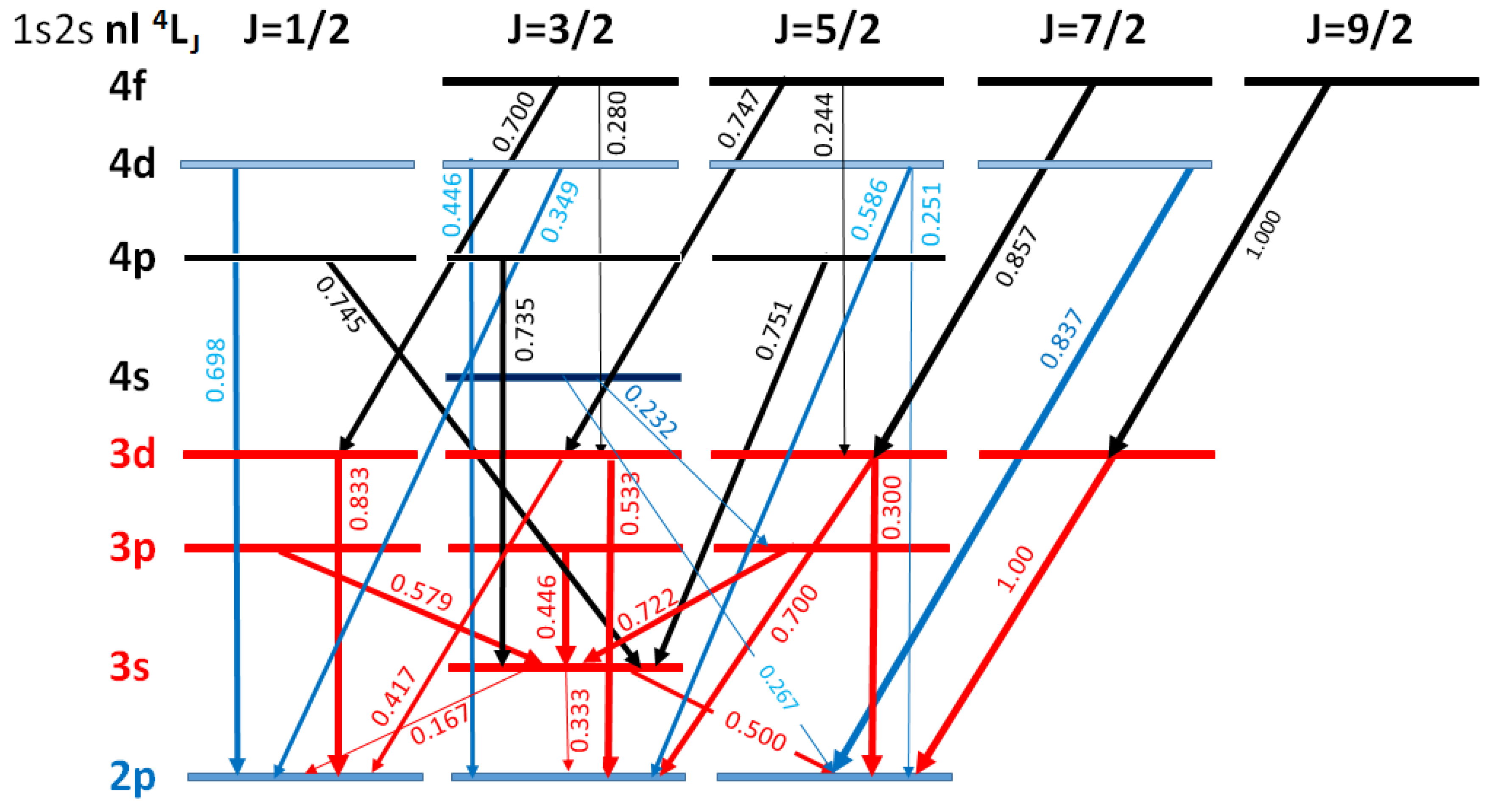
3.1. Decay Rates and Radiative Branching Ratios for C${}^{3+}\left[\left(1s2s{}^{3}S\right)n\ell {}^{4,2}L\right]$ States with $n=3$ and $n=4$

Reported atomic structure calculations on Li-like ion states including carbon have been quite prevalent. In particular, the energies of the $1s2ln{l}^{\prime }$ states for $n=2,3$ and their E1 and Auger transition rates to $1s^{2}nl$ and $1s^2$, respectively have been reported by Cheng [50] and Chen [51] using the multi-configuration Dirac-Fock method (MCDF). Also by Vainshtein and Safronova [52], Safronova and Bruch [53], and most recently by Goryaev et al. [54], using the Z-expansion method. Davis and Chung [55] presented results for the spin-induced autoionization and radiative transition rates for the $1s2s2p{}^4{P}_J$ states using the saddle-point complex rotation method. More recently, radiative and Auger transition rates also using the MCDF method, were presented for $1s2s2p{}^4{P}_J$ states by Benis et al. [56] and for $1s2s3p$ levels by Santos et al. [57].

In addition, various energy level calculations, Auger yields and line identifications of Auger transitions for Li-like carbon states have also been presented within the field of high resolution Auger projectile spectroscopy in ion-atom collisions by Schneider et al. [24,58], Mann [59], Mack and Niehaus [44], and Deveney et al. [60]. In all these publications, radiative transitions to the singly excited states $1s^{2}nl$ are only reported. However, some selective results on carbon, for radiative transitions between doubly excited states are given in Blanke et al. [61,62] (including lifetimes of $1s2pnl{}^{4}L$ states for $n=2-3$), [62] (wavelengths of $1s2s3d{}^{4}D\to 1s2s2p{}^{4}P$ transitions), Laughlin [63] (transition rates and radiative lifetimes for $1s2snl{}^{4}L$ and $1s2pnl{}^{4}L$ levels with $L\le 4$). These results do not cover all the radiative and Auger transitions needed for our cascade calculations. We therefore performed our own calculations using the COWAN code [39], to obtain the radiative and Auger transition rates and RBRs for the C${}^{3+}\left[\left(1s2s{}^{3}S\right)n\ell {}^{2,4}L\right]$ states decaying to the $1s2s{n}^{\prime }{l}^{\prime }{}^{2,4}{L}^{\prime }$ states. These results were used in our present calculations of the cascade repopulation of the $1s2s2p{}^{2,4}P$ states during the capture process.

Our calculations were carried out using the 2018 version of the COWAN [39] code, which is free of certain bugs reported earlier [64]. Our results on transition rates were compared with data from Ref. [51] for $n=2$ and $n=3$ and found in good agreement. The RCE subroutine of the code that performs the least-squares fitting of the energy levels was not used due to the lack of an adequate number of experimentally determined energy levels for the C${}^{3+}\left[\left(1s2s{}^{3}S\right)n\ell {}^{2,4}L\right]$ states.

For the autoionizing decays of the C${}^{3+}\left(1s2snl\right)$ configurations with $n\le 6$, the only allowed final state is the ground state $1s^2{}^{1}S$ of C${}^{4+}$ [41]. Thus, the Auger decay channels reported here correspond to transitions $1s2snl{}^{(2S+1)}{L}_J\to 1s^2{}^1{S}_0+e^{-}\left(l\right)$. Moreover, our results include Auger decay rates for transitions that violate spin conservation (i.e., $\Delta S\ne 0$) for the Coulomb interaction, e.g., $\left(1s2s{}^{3}S\right)3p{}^4{P}_{1/2}\to 1s^2{}^1{S}_0+e^{-}\left(p\right)$. Such transitions are attributed to the fact that the initial state of the transition is a mixed-state, i.e., it cannot be represented as a pure state in the $LS$ coupling scheme, and thus decays via a component of the mixed-state that is permitted to Auger decay [55].

Our results for the decay rates and branching ratios are presented in

Table 1. Radiative ($A_{ij}^r$) and Auger ($A_{i{f}^{\prime }}^a$) decay rates, radiative branching ratios (RBR) given by the partial fluorescence yields (${\omega }_{ij}$), and partial Auger yields (${\xi }_{i{f}^{\prime }}$) for selected transitions of the C${}^{3+}\left[\left(1s2s{}^{3}S\right)nl{}^{4}L\right]$quartet states for $n=2-4$. States are listed in order of decreasing binding energy. The lowest-lying levels (of primary interest) are separated from the rest by a double line. A “-” signifies that the computed rate leads to a negligible value (i.e., <0.1) for the related partial branching ratio and is therefore not listed.

i	Initial	j	Final ${}^{\mathit{a}}$	${\mathit{A}}_{\mathit{ij}}^{\mathit{r}}\left({\mathit{s}}^{-\mathbf{1}}\right)$	${\mathit{A}}_{{\mathit{if}}^{\prime }}^{\mathit{a}}\left({\mathit{s}}^{-\mathbf{1}}\right)$${}^{\mathit{a}}$	${\mathit{\alpha }}_{\mathit{i}}\left({\mathit{s}}^{-\mathbf{1}}\right)$	RBR—${\mathit{\omega }}_{\mathit{ij}}$	${\mathit{\xi }}_{{\mathit{if}}^{\prime }}$${}^{\mathit{a}}$
#	$\mathit{nl}{}^{\mathbf{2}\mathit{S}+\mathbf{1}}{\mathit{L}}_{\mathit{J}}$	#	$\mathit{nl}{}^{\mathbf{2}\mathit{S}+\mathbf{1}}{\mathit{L}}_{\mathit{J}}$			(Equation (2))	(Equation (4))	(Equation (5))
1	$2p{}^4{P}_{1/2}$	-	-	-	3.39 × ${10}^8$ ${}^b$	3.401 × ${10}^8$ ${}^b$	-	0.996
2	$2p{}^4{P}_{3/2}$	-	-	-	1.37 × ${10}^8$ ${}^b$	1.374 × ${10}^8$ ${}^b$	-	0.997
3	$2p{}^4{P}_{5/2}$	-	-	-	8.26 × ${10}^6$ ${}^b$	8.239 × ${10}^6$ ${}^b$	-	0.998
4	$3s{}^4{S}_{3/2}$	1	$2p{}^4{P}_{1/2}$	3.038 × ${10}^9$	-	1.820 × ${10}^{10}$	0.167	-
4		2	$2p{}^4{P}_{3/2}$	6.071 × ${10}^9$	-		0.333	-
4		3	$2p{}^4{P}_{5/2}$	9.095 × ${10}^9$	-		0.500	-
5	$3p{}^4{P}_{1/2}$	4	$3s{}^4{S}_{3/2}$	8.643 × ${10}^7$	2.730 × ${10}^7$	1.492 × ${10}^8$	0.579	0.183
6	$3p{}^4{P}_{3/2}$	4	$3s{}^4{S}_{3/2}$	1.733 × ${10}^8$	1.380 × ${10}^8$	3.886 × ${10}^8$	0.446	0.355
7	$3p{}^4{P}_{5/2}$	4	$3s{}^4{S}_{3/2}$	2.611 × ${10}^8$	-	3.615 × ${10}^8$	0.722	-
8	$3d{}^4{D}_{1/2}$	1	$2p{}^4{P}_{1/2}$	4.661 × ${10}^{10}$	-	5.595 × ${10}^{10}$	0.833	-
8		2	$2p{}^4{P}_{3/2}$	9.316 × ${10}^9$	-		0.167	-
9	$3d{}^4{D}_{3/2}$	1	$2p{}^4{P}_{1/2}$	4.661 × ${10}^{10}$	3.240 × ${10}^5$	1.119 × ${10}^{11}$	0.417	-
9		2	$2p{}^4{P}_{3/2}$	5.962 × ${10}^{10}$	-		0.533	-
9		3	$2p{}^4{P}_{5/2}$	5.584 × ${10}^9$	-		0.050	-
10	$3d{}^4{D}_{5/2}$	2	$2p{}^4{P}_{3/2}$	1.174 × ${10}^{11}$	7.590 × ${10}^5$	1.677 × ${10}^{11}$	0.700	-
10		3	$2p{}^4{P}_{5/2}$	5.026 × ${10}^{10}$	-		0.300	-
11	$3d{}^4{D}_{7/2}$	3	$2p{}^4{P}_{5/2}$	2.234 × ${10}^{11}$	-	2.235 × ${10}^{11}$	1.000	-
12	$4s{}^4{S}_{3/2}$	2	$2p{}^4{P}_{3/2}$	1.875 × ${10}^9$	-	1.051 × ${10}^{10}$	0.178	-
12		3	$2p{}^4{P}_{5/2}$	2.810 × ${10}^9$	-		0.267	-
12		6	$3p{}^4{P}_{3/2}$	1.630 × ${10}^9$	-		0.155	-
12		7	$3p{}^4{P}_{5/2}$	2.442 × ${10}^9$	-		0.232	-
13	$4p{}^4{P}_{1/2}$	4	$3s{}^4{S}_{3/2}$	1.214 × ${10}^9$	1.280 × ${10}^7$	1.630 × ${10}^9$	0.745	-
13		8	$3d{}^4{D}_{1/2}$	1.866 × ${10}^8$	-		0.114	-
13		9	$3d{}^4{D}_{3/2}$	1.866 × ${10}^8$	-		0.114	-
14	$4p{}^4{P}_{3/2}$	4	$3s{}^4{S}_{3/2}$	2.427 × ${10}^9$	6.460 × ${10}^7$	3.302 × ${10}^9$	0.735	-
14		10	$3d{}^4{D}_{5/2}$	4.703 × ${10}^8$	-		0.142	-
15	$4p{}^4{P}_{5/2}$	4	$3s{}^4{S}_{3/2}$	3.642 × ${10}^9$	-	4.850 × ${10}^9$	0.751	-
15		11	$3d{}^4{D}_{7/2}$	8.960 × ${10}^8$	-		0.185	-
16	$4d{}^4{D}_{1/2}$	1	$2p{}^4{P}_{1/2}$	1.614 × ${10}^{10}$	-	2.314 × ${10}^{10}$	0.698	-
16		2	$2p{}^4{P}_{3/2}$	3.225 × ${10}^9$	-		0.139	-
16		5	$3p{}^4{P}_{1/2}$	3.141 × ${10}^9$	-		0.136	-
17	$4d{}^4{D}_{3/2}$	1	$2p{}^4{P}_{1/2}$	1.614 × ${10}^{10}$	1.560 × ${10}^5$	4.626 × ${10}^{10}$	0.349	-
17		2	$2p{}^4{P}_{3/2}$	2.064 × ${10}^{10}$	-		0.446	-
18	$4d{}^4{D}_{5/2}$	2	$2p{}^4{P}_{3/2}$	4.064 × ${10}^{10}$	3.640 × ${10}^5$	6.936 × ${10}^{10}$	0.586	-
18		3	$2p{}^4{P}_{5/2}$	1.740 × ${10}^{10}$	-		0.251	-
18		6	$3p{}^4{P}_{3/2}$	7.911 × ${10}^9$	-		0.114	-
19	$4d{}^4{D}_{7/2}$	3	$2p{}^4{P}_{5/2}$	7.735 × ${10}^{10}$	-	9.243 × ${10}^{10}$	0.837	-
19		7	$3p{}^4{P}_{5/2}$	1.506 × ${10}^{10}$	-		0.163	-
20	$4f{}^4{F}_{3/2}$	8	$3d{}^4{D}_{1/2}$	1.153 × ${10}^{10}$	-	1.647 × ${10}^{10}$	0.700	-
20		9	$3d{}^4{D}_{3/2}$	4.614 × ${10}^9$	-		0.280	-
21	$4f{}^4{F}_{5/2}$	9	$3d{}^4{D}_{3/2}$	1.845 × ${10}^{10}$	7.060 × ${10}^4$	2.471 × ${10}^{10}$	0.747	-
21		10	$3d{}^4{D}_{5/2}$	6.025 × ${10}^9$	-		0.244	-
22	$4f{}^4{F}_{7/2}$	10	$3d{}^4{D}_{5/2}$	2.824 × ${10}^{10}$	1.290 × ${10}^5$	3.295 × ${10}^{10}$	0.857	-
22		11	$3d{}^4{D}_{7/2}$	4.706 × ${10}^9$	-		0.143	-
23	$4f{}^4{F}_{9/2}$	11	$3d{}^4{D}_{7/2}$	4.118 × ${10}^{10}$	-	4.118 × ${10}^{10}$	1.000	-

${}^a$ All Auger transitions refer to the same final ionic state $f^{\prime }$, i.e., C${}^{4+}\left(1s^2{}^1{S}_0\right)$.; ${}^b$ From Benis et al. [56].

for the quartet and

Table 2. Same as Table 1, but for the C${}^{3+}\left[\left(1s2s{}^{3,1}S\right)nl{}^{2}L\right]$doublet states. Shorthand: $n{l}^2{L}_{-J}\equiv \left(1s2s{}^{3}S\right)nl{}^2{L}_J$ and $n{l}^2{L}_{+J}\equiv \left(1s2s{}^{1}S\right)nl{}^2{L}_J$. Here we only list states with the largest radiative rates, as well as a few other indicative connecting ones. In most cases, the RBR is much smaller than 0.022, marked by "-" and considered negligible.

i	Initial	j	Final ${}^{\mathit{a}}$	${\mathit{A}}_{\mathit{ij}}^{\mathit{r}}\left({\mathit{s}}^{-\mathbf{1}}\right)$	${\mathit{A}}_{{\mathit{ij}}^{\prime }}^{\mathit{a}}{\left({\mathit{s}}^{-\mathbf{1}}\right)}^{\mathit{a}}$	${\mathit{\alpha }}_{\mathit{i}}\left({\mathit{s}}^{-\mathbf{1}}\right)$	RBR—${\mathit{\omega }}_{\mathit{ij}}$	${\mathit{\xi }}_{{\mathit{ij}}^{\prime }}$${}^{\mathit{a}}$
#	$\mathit{nl}{}^{\mathbf{2}\mathit{S}+\mathbf{1}}{\mathit{L}}_{\mathit{J}}$	#	$\mathit{nl}{}^{\mathbf{2}\mathit{S}+\mathbf{1}}{\mathit{L}}_{\mathit{J}}$			(Equation (2))	(Equation (4))	(Equation (5))
1	$2p{}^2{P}_{-1/2}$	-	-	-	1.47 × ${10}^{13}$ ${}^b$	1.52 × ${10}^{13}$ ${}^b$	-	0.968
2	$2p{}^2{P}_{-3/2}$	-	-	-	1.43 × ${10}^{13}$ ${}^b$	1.48 × ${10}^{13}$ ${}^b$	-	0.967
3	$2p{}^2{P}_{+1/2}$	-	-	-	3.86 × ${10}^{13}$ ${}^b$	3.87 × ${10}^{13}$ ${}^b$	-	0.998
4	$2p{}^2{P}_{+3/2}$	-	-	-	3.86 × ${10}^{13}$ ${}^b$	3.87 × ${10}^{13}$ ${}^b$	-	0.998
5	$3s{}^2{S}_{-1/2}$	1	$2p{}^2{P}_{-1/2}$	2.954 × ${10}^8$	2.380 × ${10}^{13}$	2.381 × ${10}^{13}$	-	1.00
5		2	$2p{}^2{P}_{-3/2}$	5.795 × ${10}^8$			-
5		3	$2p{}^2{P}_{+1/2}$	1.734 × ${10}^9$			-
5		4	$2p{}^2{P}_{+3/2}$	3.482 × ${10}^9$			-
6	$3s{}^2{S}_{+1/2}$	3	$2p{}^2{P}_{+1/2}$	2.084 × ${10}^9$	1.380 × ${10}^{13}$	1.382 × ${10}^{13}$	-	0.999
7	$3p{}^2{P}_{-1/2}$	6	$3s{}^2{S}_{+1/2}$	1.561 × ${10}^7$	5.130 × ${10}^{12}$	5.494 × ${10}^{12}$	-	0.934
8	$3p{}^2{P}_{-3/2}$	5	$3s{}^2{S}_{-1/2}$	3.107 × ${10}^7$	1.030 × ${10}^{13}$	1.103 × ${10}^{13}$	-	0.934
9	$3p{}^2{P}_{+1/2}$	6	$3s{}^2{S}_{+1/2}$	4.573 × ${10}^7$	1.880 × ${10}^{13}$	1.893 × ${10}^{13}$	-	0.993
10	$3p{}^2{P}_{+3/2}$	6	$3s{}^2{S}_{+1/2}$	9.235 × ${10}^7$	3.760 × ${10}^{13}$	3.785 × ${10}^{13}$	-	0.993
11	$3d{}^2{D}_{-3/2}$	3	$2p{}^2{P}_{+1/2}$	4.768 × ${10}^{10}$	5.690 × ${10}^{11}$	6.751 × ${10}^{11}$	0.071	0.843
12	$3d{}^2{D}_{-5/2}$	4	$2p{}^2{P}_{+3/2}$	8.646 × ${10}^{10}$	8.540 × ${10}^{11}$	1.013 × ${10}^{12}$	0.085	0.843
13	$3d{}^2{D}_{+3/2}$	1	$2p{}^2{P}_{-1/2}$	4.480 × ${10}^{10}$	1.830 × ${10}^{12}$	1.937 × ${10}^{12}$	0.023	0.945
14	$3d{}^2{D}_{+5/2}$	2	$2p{}^2{P}_{-3/2}$	8.120 × ${10}^{10}$	2.740 × ${10}^{12}$	2.901 × ${10}^{12}$	0.028	0.945
15	$4s{}^2{S}_{-1/2}$	4	$2p{}^2{P}_{+3/2}$	1.716 × ${10}^9$	9.530 × ${10}^{12}$	9.536 × ${10}^{12}$	-	0.999
16	$4s{}^2{S}_{+1/2}$	4	$2p{}^2{P}_{+3/2}$	1.920 × ${10}^9$	4.780 × ${10}^{12}$	4.792 × ${10}^{12}$	-	0.997
17	$4p{}^2{P}_{-3/2}$	5	$3s{}^2{S}_{-1/2}$	3.251 × ${10}^9$	4.020 × ${10}^{12}$	4.369 × ${10}^{12}$	-	0.920
18	$4p{}^2{P}_{+3/2}$	6	$3s{}^2{S}_{+1/2}$	2.667 × ${10}^9$	1.510 × ${10}^{13}$	1.519 × ${10}^{13}$	-	0.994
19	$4d{}^2{D}_{-3/2}$	1	$2p{}^2{P}_{-1/2}$	1.865 × ${10}^{10}$	2.130 × ${10}^{11}$	2.627 × ${10}^{11}$	0.071	0.811
20	$4d{}^2{D}_{-5/2}$	4	$2p{}^2{P}_{+3/2}$	2.507 × ${10}^{10}$	3.190 × ${10}^{11}$	3.936 × ${10}^{11}$	0.064	0.810
21	$4d{}^2{D}_{+3/2}$	3	$2p{}^2{P}_{+1/2}$	2.477 × ${10}^{10}$	1.040 × ${10}^{12}$	1.084 × ${10}^{12}$	0.022	0.960
22	$4d{}^2{D}_{+5/2}$	4	$2p{}^2{P}_{+3/2}$	4.442 × ${10}^{10}$	1.550 × ${10}^{12}$	1.615 × ${10}^{12}$	0.028	0.960
23	$4f{}^2{F}_{-5/2}$	11	$3d{}^2{D}_{-3/2}$	2.081 × ${10}^{10}$	5.170 × ${10}^9$	2.835 × ${10}^{10}$	0.734	0.182
24	$4f{}^2{F}_{-7/2}$	12	$3d{}^2{D}_{-5/2}$	2.973 × ${10}^{10}$	6.890 × ${10}^9$	3.780 × ${10}^{10}$	0.787	0.182
25	$4f{}^2{F}_{+5/2}$	13	$3d{}^2{D}_{+3/2}$	2.241 × ${10}^{10}$	6.550 × ${10}^9$	3.186 × ${10}^{10}$	0.703	0.206
26	$4f{}^2{F}_{+7/2}$	14	$3d{}^2{D}_{+5/2}$	3.201 × ${10}^{10}$	8.730 × ${10}^9$	4.247 × ${10}^{10}$	0.754	0.206

${}^a$ All Auger transitions refer to the same final ionic state, i.e., C${}^{4+}\left(1s^2{}^1{S}_0\right)$; ${}^b$ From Chen [51].

for the doublet states, respectively. Transitions with RBRs smaller than $0.1$ are considered negligible and omitted. Based on these results, a Grotrian diagram of the strongest quartet transitions for the carbon $1s2snl{}^4{L}_J$ states with $n\le 4$ is shown in Figure 3.

3.2. Cascade Feeding Considerations

As seen in Table 1 and more clearly in the Grotrian diagram of Figure 3 for the quartets, there are higher-lying levels where the RBR ${\omega }_{ij}$ is close to 1. On the other hand, in Table 2 for the doublets, the computed RBRs are mostly very small making cascade feeding negligible. This is consistent with previous cascade repopulation findings for Li-like carbon [34,35] and fluorine [33] states populated by $nl$ SEC (Equation (36)). Therefore, in the case of the doublets, no cascade calculations were performed. Thus, cascade feeding calculations were only performed for the quartet states.

In general, for the quartets, the Auger rates $A_{i{f}^{\prime }}^a$ decrease in strength as the principal quantum number n increases, while the radiative rates $A_{ij}^r$ increase. Thus, the higher-lying levels are seen to have increased RBRs compared to levels below them, increasing the cascade feeding probability of the lowest-lying $2p{}^4{P}_J$ levels (i.e., with $J=1/2,3/2,5/2$) of interest. Of special interest are also the Yrast states (those with maximal J within the same $nl{}^{4}L$ level), as already pointed out by Schneider et al [24], which can provide a path of maximal cascade probability. Indeed, we note that the Yrast cascade chain $4f{}^4{F}_{9/2}\to 3d{}^4{D}_{7/2}\to 2p{}^4{P}_{5/2}$ (or in Table 1 level numbers $23\to 11\to 3$) all have the strongest RBRs ${\omega }_{if}=1$ along this path (e.g., ${\omega }_{23,11}={\omega }_{11,3}$ = 1) and therefore a 2nd-order ($c_2$) cascade probability of 1 (${\omega }_{23,11}·{\omega }_{11,3}$ = 1).

For the doublets, even though there are RBRs with large ${\omega }_{ij}$ values as listed in Table 2 for $n=4$ (e.g., the Yrast transition $4f{}^2{F}_{-7/2}\to 3d{}^2{D}_{-5/2}$, has ${\omega }_{24,12}=0.787$), their follow up transition feeding the levels of interest are seen to be much weaker (e.g., the transition $3d{}^2{D}_{-5/2}\to 2p{}^2{P}_{+1/2}$, has only ${\omega }_{12,3}=0.085$), effectively resulting in a negligible overall $c_2$ cascade probability (e.g., $0.787·0.085=0.067$).

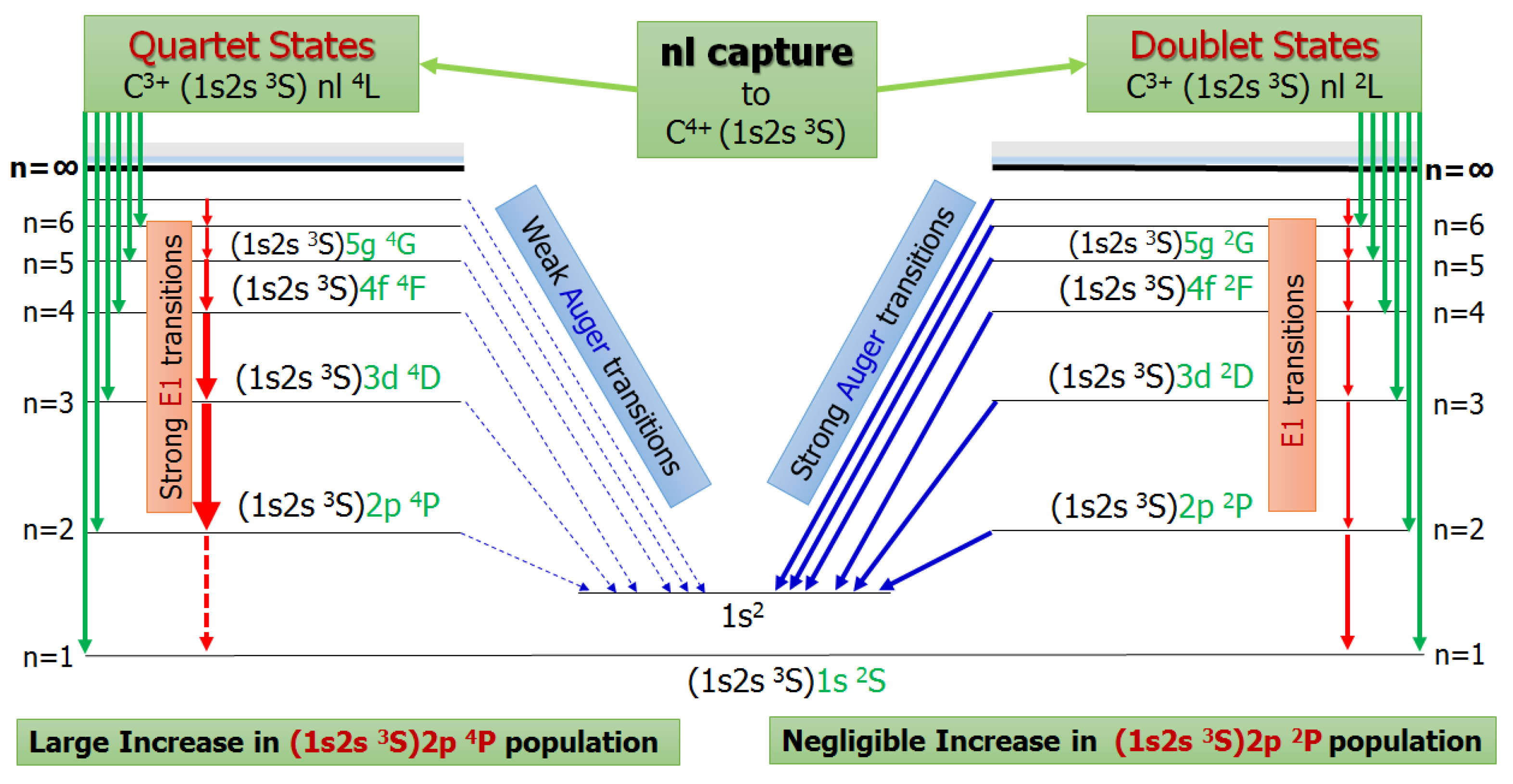
3.3. Initial State Populations

The same initial state populations (cross sections ${\mathcal{S}}^{c_0}\left(E_p\right)$ in Equation (33)) were used as used in Ref. [30]. These were computed in [30] for $2p$ SEC using ab initio dynamical calculations involving three active electrons within a full configuration interaction approach. This involved a semiclassical atomic orbital close-coupling calculation (referred to as 3eAOCC), with asymptotic descriptions of the atomic collision partners [65,66,67]: the time-dependent Schrödinger equation was solved non-perturbatively, with the inclusion of all couplings related to the static and dynamic interelectronic repulsions and effects stemming from the Pauli exclusion principle. This approach allows for the accurate modeling of the C${}^{4+}$ and C${}^{3+}$ electronic structures, including spin and spatial components. It also describes the dynamics of the system, inducing among other things, excitation, ionization (through population of pseudo states [67]) and capture to singly and doubly excited states on the carbon center. Overall, this 3eAOCC approach goes much beyond frozen core models advocated in the past [34,35], where only one active electron is considered in the dynamics4. SEC cross sections to higher-lying $1s2snl{}^{4}L$ states for $n=3-4$ were also computed by our close-coupling treatment. Finally, the He target was described by a model potential binding just a single electron to He${}^{+}$ with the appropriate He$\left(1s^2\right)$ energies4.

Using these initial state cross sections, the calculated ratio R was found in good agreement with experiment, for the first time, when the radiative cascades were also taken into account. These results on R, presented in [30], resolved the previously existing disagreement between theory and experiment [34,35], while underlining the limited predictive power of the frozen core approximation as regards to spin statistics in such highly correlated dynamical atomic systems.

4. Results and Discussion

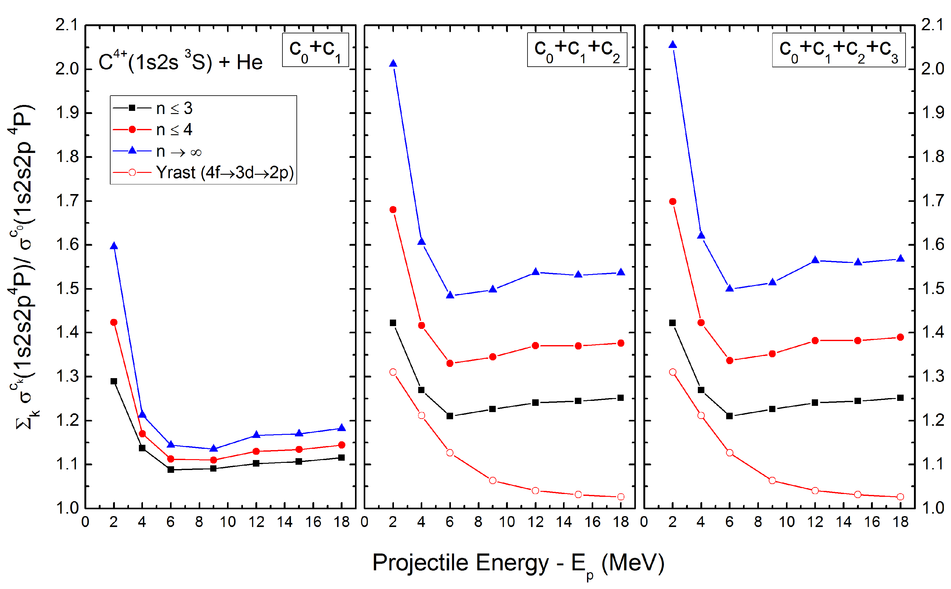
In this work, we implement the cascade matrix formulation (i.e., Equation (34)), progressively computing increasing cascade order contributions to obtain the overall cascade repopulation of the states of interest. This requires the independent calculation of: (i) the initial SEC production cross sections, and (ii) the necessary RBRs ${\omega }_{ij}$. Since, as already mentioned, intercombination transitions are very weak, the cascade calculations are typically done separately for each spin symmetry (i.e., quartet or doublet). Due to the much smaller doublet RBRs (compared to the corresponding quartet RBRs), as evident in Table 2, the cascade repopulation of the doublets will be insignificant, consistent with previously reported results [35], and is therefore not performed. Thus, only cascade repopulation of the quartet states is considered here. This is performed using an $\tilde{\Omega }[M=23\times M=23]$ cascade matrix with entries ${\tilde{\omega }}_{ji}={\omega }_{ij}$, as listed in Table 1.

4.1. Cascade Enhancement of the $1s2s2p{}^{4}P$ Level Population and Contributing Cascade Orders

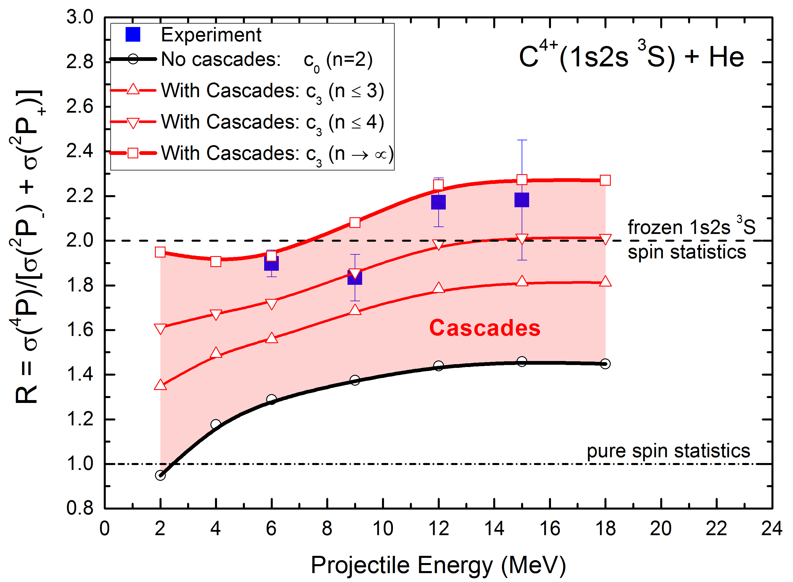
In Figure 4, we plot, as a function of the collision energy $E_p$, the ratio of progressive cascade contributions $c_1$, $c_2$, and $c_3$ to $c_0$ for the $1s2s2p{}^{4}P$ state due to higher-lying $1s2sn\ell {}^{4}L$ populations with increasing principal quantum number n.

These results are then extrapolated to $n\to \infty$, using an $n^{-3}$ SEC population model [34,45]. From Figure 4, it is evident, that depending on collision energy $E_p$, the first cascade order $c_1$, accounts for an increase of about 10–30% for transitions just from the $n=3$ levels. This is consistent with the Grotrian diagram in Figure 3, where most $n=3$ RBRs are seen to be large. Furthermore, the second cascade order, $c_2$, for both $n=3$ and $n=3+4$, as well as the extrapolation to include all n, are even more important accounting for a further increase of 10–40%. Finally, including also cascade contributions $c_3$, only a very small increase is observed with decreasing collision energy, as SEC to higher-lying n levels becomes more important [44]. Also shown, is the contribution of the Yrast cascade sequence also seen to become increasingly important with decreasing collision energy.

4.2. Spin Statistics—Ratio R of $1s2s2p$ ${}^{4}P$ to ${}^{2}P$ Cross Sections

In our recent publication [30], the long-standing problem of how multi-unpaired-electron ion cores behave, while undergoing electron processes during fast atomic collisions, was treated both experimentally and theoretically. A viable way to explore this is to consider the $2p$ SEC channel in MeV collisions (Equation (36)). There, the ratio R of the similarly configured $1s2s2p$ ${}^{4}P$ to ${}^2{P}_{\pm }$ SEC cross sections, defined by Equation (37), should bear the corresponding population spin statistics signature. This ratio should have the value of $R=1$ when considering only spin multiplicity, or the value $R=2$, in the frozen core approximation, where only the ${}^{4}P$ and a single ${}^{2}P$ states can be produced by SEC from the $1s2s{}^{3}S$ initial state [34,36,37]. Experimental investigations involved beams of C${}^{4+}(1s^2,1s2s{}^{3}S)$ mixed-state ions, prepared with different amounts of metastable $1s2s{}^{3}S$ component. Then, the ratio R could be evaluated by applying our two-spectra technique for the proper determination of the contributions from just the $1s2s{}^{3}S$ beam component [43]. The measurements were performed using the ZAPS [46] setup, currently located at the NCSR “Demokritos” 5.5 MV Tandem accelerator facility in Athens [68]. The corresponding theoretical investigations were performed in Paris using the above mentioned 3eAOCC calculations involving the dynamics of three active electrons within a full configuration interaction approach [66].

Based on the above 3eAOCC and cascade calculations, the ratio R of the SEC cross sections of the quartet $1s2s2p{}^{4}P$ (for short ${}^{4}P$) to doublet $1s2s2p{}^2{P}_{\pm }$ (for short ${}^2{P}_{\pm }$) is given by:

$$\begin{array}{cc}\hfill R& \equiv \frac{\sigma {(}^{4}P)}{\sigma {(}^2{P}_{-})+\sigma {(}^2{P}_{+})}=\frac{{\sigma }^{c_0}{(}^{4}P)+{\sigma }^{c_1}{(}^{4}P)+{\sigma }^{c_2}{(}^{4}P)+{\sigma }^{c_3}{(}^{4}P)}{{\sigma }^{c_0}{(}^2{P}_{-})+{\sigma }^{c_0}{(}^2{P}_{+})},\hfill \end{array}$$

(37)

where the cross sections ${\sigma }^{c_k}\left(X\right)$ correspond to the sum of the cross sections of all levels i related to the same term X, e.g., ${\sigma }^{c_3}{(}^{4}P)={\sigma }^{c_3}{(}^4{P}_{1/2})+{\sigma }^{c_3}{(}^4{P}_{3/2})+{\sigma }^{c_3}{(}^4{P}_{5/2})$, i.e., the $c_3$ cascade contributions to levels $i=1-3$ according to Table 1.

R was computed up to and including third order cascades, $c_3$, according to the formulation of Equation (34). Results are shown in Figure 5, along with the ZAPS measurements reported in [30]. Here, we increased the number of electron configurations from 20 to 29 in the COWAN code5 obtaining slightly smaller values for R compared to the ones previously reported [30], which resulted in improved agreement with experiment as seen in Figure 5.

These and our previous results [30], essentially invalidate the frozen core approximation commonly used in the past (e.g., Röhrbein et al. [35], found much larger values of the ratio R with or without cascades) when considering electron capture in multi-electron, multi-open-shell quantum systems [30]. While the frozen $1s2s{}^{3}S$ spin statistic limit shown in Figure 5 with the value of 2 [37], does indeed seem to agree with our experimental data, it does not include cascades. These have been shown by us (and Röhrbein et al. [35] before us) to be important, lifting this limit of 2 to about 3.5 (minimum), when including cascade repopulation as calculated here.

4.3. Comparison to Older Cascade Calculations on the C${}^{4+}\left(1s2s{}^{3}S\right)+$ He Collision System

Finally, we should also mention the two previous cascade calculations for the same C${}^{4+}\left(1s2s{}^{3}S\right)+$ He collision system reported by Strohschein et al. [34] and Röhrbein et al. [35]. In Ref. [34], the cascade calculations ignored the Auger channel. Thus, the decay constant ${\alpha }_n$ in Equation (2) included only radiative rates and was therefore smaller than when Augers are included. This was corrected in Ref. [35], where the full ${\alpha }_n$ decay constants were used, thus also properly including the Auger decays. In the former ${}^{4}P$ calculation [34], since the ${}^{4}P$ Auger decay rate is small compared to the inter-quartet $E1$ radiative transitions rates, the RBR is not much affected by the non-inclusion of the Auger channel, so the selective enhancement of the ${}^{4}P$ remained substantial [34]. However, neglecting the Auger channel in the calculation of the doublets is a much stronger effect since here the RBRs change substantially [35]. This can be readily seen in our calculated doublet rates shown in Table 2. For example, for the initial level $\left(1s2s{}^{3}S\right)3d{}^2{D}_{5/2}$, referred to in the table as level 12 ($3d{}^2{D}_{-5/2}$), ${\alpha }_{12}=1.013\times {10}^{12}$ s${}^{-1}$ including the Auger channel, while equal to $1.013\times {10}^{12}-8.540\times {10}^{11}=1.590\times {10}^{11}$ s${}^{-1}$ without, with corresponding RBR ${\omega }_{12,4}=8.646\times {10}^{10}/1.103\times {10}^{12}=0.0854$ with the Auger channel, and ${\omega }_{12,4}=8.646\times {10}^{10}/1.590\times {10}^{11}=0.5438$ without (a huge difference).

In addition to these atomic structure considerations, in both previous calculations, the initial SEC populations were calculated within a one-active-electron frozen core treatment using the two-center basis generator method (TC-BGM) [35]. This gave a ratio $R\approx 2$ without cascades, very different from the value of $R\approx 1.1-1.4$ reported by us [30], using the 3eAOCC approach. Furthermore, the cascade contributions to R were found to increase its value by a factor of ≲2.9 (see Figure 6 in Ref. [35]), while in our calculation [30], as also shown here, the increase due to cascades in R is smaller, at about a factor ∼1.6 (see Figure 5). These differences between the two results, can be readily attributed in both cases (i.e., R with and without cascade contributions) to the present use of a dynamic approach involving several active correlated electrons, avoiding the constraints of the $1s2s{}^{3}S$ frozen core approximation required in one-electron treatments [30].

5. Summary and Conclusions

We have theoretically investigated radiative cascade repopulation of the C${}^{3+}\left(1s2s2p\right)$ ${}^{4}P$ quartet and ${}^{2}P$ doublet states formed in 2–18 MeV collisions of C${}^{4+}\left(1s2s{}^{3}S\right)$ ions with He gas target. Using the diagrammatic cascade formalism of Curtis [38], after including also the Auger decay of the doubly excited states, we have integrated the rate equations over long-enough time ($t\to \infty$) to obtain the final level populations including cascade repopulation. Results are calculated analytically within a straight-forward cascade matrix approach and the contributions of each cascade order to the cross sections are readily computed, as described in detail.

To initiate the cascade calculations, the $t=0$ initial populations of the $1s2sn\ell {}^{4}L$, $1s2sn\ell {}^{2}L$ levels included in our analysis are obtained from the direct $n\ell$ single electron capture (SEC) cross sections previously computed in Ref. [30], using the novel three-electron close-coupling (3eAOCC) approach.

Our cascade matrix includes all relevant radiative branching ratios (RBR) for $n\le 4$ computed using the COWAN atomic structure code. In the case of the doublets, the RBRs are found to be very small (<0.1) showing that cascade feeding in this case, can be neglected, consistent with previous results by other groups [35]. In the case of the quartets though, the RBRs are found to be large, in some cases equal to 1. Cascade calculations (extrapolated to $n\to \infty$ using an $n^{-3}$ SEC model) were then performed including up to third order cascades, which showed an up to 60% increase of the $1s2s2p{}^{4}P$ population due to cascades. Using these cascade calculations including initial level populations provided by our independently calculated cross sections, we computed the ratio R of $1s2s2p$ ${}^{4}P$ to ${}^{2}P$ cross sections including cascades, of recent spin statistics interest [30,33,34,35], and found it in good agreement with experiment.

Future systematic isoelectronic investigations of the spin statistics ratio R would be of great interest to further validate our conclusions in a more general context. Cascade calculations will therefore also be important, particularly at the lowest collision energies where SEC to higher-lying levels is strongest.

References

1. Beiersdorfer, P. Laboratory X-ray Astrophysics. Annu. Rev. Astron. Astrophys. 2003, 41, 343–390. [Google Scholar] [CrossRef]
2. Shevelko, V.; Tawara, H. (Eds.) Atomic Processes in Basic and Applied Physics; Springer: Berlin/Heidelberg, Germany; New York, NY, USA, 2012. [Google Scholar]
3. Osterbrock, D.E.; Ferland, G.J. Astrophysics of Gaseous Nebulae and Active Galactic Nuclei; University Science Books: Mill Valley, CA, USA, 2006. [Google Scholar]
4. Pradhan, A.K.; Nahar, S.N. Atomic Astrophysics and Spectroscopy; Cambridge University Press: Cambridge, UK, 2011. [Google Scholar]
5. Bureyeva, L.A.; Lisitsa, V.S.; Namba, C.; Shuvaev, D.A. Radiative cascade following dielectronic recombination. J. Phys. B 2002, 35, 2505–2514. [Google Scholar] [CrossRef]
6. Cumbee, R.S.; Mullen, P.D.; Lyons, D.; Shelton, R.L.; Fogle, M.; Schultz, D.R.; Stancil, P.C. Charge Exchange X-ray Emission due to Highly Charged Ion Collisions with H, He, and H2: Line Ratios for Heliospheric and Interstellar Applications. Astrophys. J. 2017, 852, 7. [Google Scholar] [CrossRef]
7. Fritzsche, S. A fresh computational approach to atomic structures, processes and cascades. Comput. Phys. Commun. 2019, 240, 1–14. [Google Scholar] [CrossRef]
8. Hahn, Y.; Lagattuta, K.J. Dielectronic recombination and related resonance processes. Phys. Rep. 1988, 166, 195–268. [Google Scholar] [CrossRef]
9. Pradhan, A.K. Recombination-cascade X-ray spectra of highly charged helium-like ions. Astrophys. J. 1985, 288, 824–830. [Google Scholar] [CrossRef]
10. Kabachnik, N.M.; Fritzsche, S.; Grum-Grzhimailo, A.N.; Meyer, M.; Ueda, K. Coherence and correlations in photoinduced Auger and fluorescence cascades in atoms. Phys. Rep. 2007, 451, 155–233. [Google Scholar] [CrossRef]
11. Loch, S.D.; Pindzola, M.S.; Ballance, C.P.; Griffin, D.C. The effects of radiative cascades on the X-ray diagnostic lines of Fe16+. J. Phys. B 2006, 39, 85–104. [Google Scholar] [CrossRef] [Green Version]
12. Mirakhmedov, M.N.; Parilis, E.S. Auger and X-ray cascades following inner-shell ionisation. J. Phys. B 1988, 21, 795–804. [Google Scholar] [CrossRef]
13. Pepino, R.; Kharchenko, V.; Dalgarno, A.; Lallement, R. Spectra of the X-ray Emission Induced in the Interaction between the Solar Wind and the Heliospheric Gas. Astrophys. J. 2004, 617, 1347–1352. [Google Scholar] [CrossRef]
14. Trassinelli, M.; Prigent, C.; Lamour, E.; Mezdari, F.; Mérot, J.; Reuschl, R.; Rozet, J.P.; Steydli, S.; Vernhet, D. Investigation of slow collisions for (quasi) symmetric heavy systems: What can be extracted from high resolution X-ray spectra. J. Phys. B 2012, 45, 085202. [Google Scholar] [CrossRef]
15. Tawara, H.; Richard, P.; Safronova, U.I.; Stancil, P.C. K X-ray production in H-like Si13+, S15+, and Ar17+ ions colliding with various atom and molecule gas targets at low collision energies. Phys. Rev. A 2001, 64, 042712. [Google Scholar] [CrossRef]
16. Tawara, H.; Richard, P.; Safronova, U.I.; Stancil, P.C. Erratum. Phys. Rev. A 2002, 65, 059901. [Google Scholar] [CrossRef]
17. Astner, G.; Curtis, L.J.; Liljeby, L.; Mannervik, S.; Martinson, I. A high precision beam-foil meanlife measurement of the 1s3p1P level in He I. Zeitschrift Phys. A 1976, 279, 1–6. [Google Scholar] [CrossRef]
18. Träbert, E. Beam–foil spectroscopy—Quo vadis? Physica Scr. 2008, 78, 038103. [Google Scholar] [CrossRef]
19. Curtis, L.J. Beam Foil Spectroscopy; Bashkin, S., Ed.; Springer: Berlin, Germany, 1976; p. 63. [Google Scholar]
20. Charalambidis, D.; Brenn, R.; Koulen, K.J. Transition rates of 1s2s2p 4 P J o states of Li-like ions (Z = 8, 7, 6). Phys. Rev. A 1989, 40, 2359–2364. [Google Scholar] [CrossRef]
21. Träbert, E. Radiative-Lifetime measurements on highly charged Ions. In Accelerator-Based Atomic Physics: Techniques and Applications; Shafroth, S.M., Austin, J.C., Eds.; AIP: Woodbury, NY, USA, 1997; pp. 567–607, Chapter 17. [Google Scholar]
22. Träbert, E. In pursuit of highly accurate atomic lifetime measurements of multiply charged ions. J. Phys. B 2010, 43, 074034. [Google Scholar] [CrossRef] [Green Version]
23. Martinson, I. Mean life studies in light atoms. Nucl. Instrum. Methods 1970, 90, 81–84. [Google Scholar] [CrossRef]
24. Schneider, D.; Bruch, R.; Schwarz, W.H.E.; Chang, T.C.; Moore, C.F. Identifications of Auger spectra from 2-MeV foil-excited carbon ions. Phys. Rev. A 1977, 15, 926–934. [Google Scholar] [CrossRef]
25. Sellin, I.A.; Pegg, D.J.; Brown, M.; Smith, W.W.; Donnally, B. Spectra of Autoionization Electrons Emitted by Fast, Metastable Beams of Highly Stripped Oxygen and Fluorine Ions. Phys. Rev. Lett. 1971, 27, 1108–1111. [Google Scholar] [CrossRef]
26. Donnally, B.; Smith, W.W.; Pegg, D.J.; Brown, M.; Sellin, I.A. Lifetimes of the Metastable Auto-Ionizing (1s2s2p)4P5/2 States of Lithiumlike F6+ and O5+ Ions. Phys. Rev. A 1971, 4, 122–125. [Google Scholar] [CrossRef]
27. Berry, H.G.; Pinnington, E.H.; Subtil, J.L. Energies and Mean Lives of Doubly Excited Terms in Lithium. J. Opt. Soc. Am. 1972, 62, 767–771. [Google Scholar] [CrossRef]
28. Sellin, I.A.; Pegg, D.J.; Griffin, P.M.; Smith, W.W. Metastable Autoionizing States of Highly Excited Heavy Ions. Phys. Rev. Lett. 1972, 28, 1229–1232. [Google Scholar] [CrossRef]
29. Mannervik, S. Optical studies of multiply excited states. Physica Scr. 1989, 40, 28–52. [Google Scholar] [CrossRef]
30. Madesis, I.; Laoutaris, A.; Zouros, T.J.M.; Benis, E.P.; Gao, J.W.; Dubois, A. Pauli Shielding and Breakdown of Spin Statistics in Multielectron Multi-Open-Shell Dynamical Atomic Systems. Phys. Rev. Lett. 2020, 124, 113401. [Google Scholar] [CrossRef]
31. Tanis, J.A.; Landers, A.L.; Pole, D.J.; Alnaser, A.S.; Hossain, S.; Kirchner, T. Evidence for Pauli Exchange Leading to Excited-State Enhancement in Electron Transfer. Phys. Rev. Lett. 2004, 92, 133201. [Google Scholar] [CrossRef] [Green Version]
32. Tanis, J.A.; Landers, A.L.; Pole, D.J.; Alnaser, A.S.; Hossain, S.; Kirchner, T. Erratum. Phys. Rev. Lett. 2006, 96, 019901. [Google Scholar] [CrossRef]
33. Zouros, T.J.M.; Sulik, B.; Gulyás, L.; Tökési, K. Selective enhancement of 1s2s2p 4PJ metastable states populated by cascades in single-electron transfer collisions of F7+ (1s2/1s2s 3S) ions with He and H2 targets. Phys. Rev. A 2008, 77, 050701. [Google Scholar] [CrossRef]
34. Strohschein, D.; Röhrbein, D.; Kirchner, T.; Fritzsche, S.; Baran, J.; Tanis, J.A. Nonstatistical enhancement of the 1s2s2p 4P state in electron transfer in 0.5–1.0-MeV/u C4,5+ + He and Ne collisions. Phys. Rev. A 2008, 77, 022706. [Google Scholar] [CrossRef]
35. Röhrbein, D.; Kirchner, T.; Fritzsche, S. Role of cascade and Auger effects in the enhanced population of the C3+ (1s2s2p 4P) states following single-electron capture in C4+ (1s2s 3S)-He collisions. Phys. Rev. A 2010, 81, 042701. [Google Scholar] [CrossRef]
36. Benis, E.P.; Zouros, T.J.M.; Gorczyca, T.W.; González, A.D.; Richard, P. Elastic resonant and nonresonant differential scattering of quasifree electrons from B4+(1s) and B3+(1s2) ions. Phys. Rev. A 2004, 69, 052718. [Google Scholar] [CrossRef]
37. Benis, E.P.; Zouros, T.J.M.; Gorczyca, T.W.; González, A.D.; Richard, P. Erratum. Phys. Rev. A 2006, 73, 029901. [Google Scholar] [CrossRef]
38. Curtis, L.J. A Diagrammatic Mnemonic for Calculation of Cascading Level Populations. Am. J. Phys. 1968, 36, 1123–1125. [Google Scholar] [CrossRef]
39. Cowan, R.D. The Theory of Atomic Structure and Spectra; University of California Press: Berkeley, CA, USA, 1981. [Google Scholar]
40. Shiina, Y.; Kinoshita, R.; Funada, S.; Matsuda, M.; Imai, M.; Kawatsura, K.; Sataka, M.; Sasa, K.; Tomita, S. Measurement of Auger electrons emitted through Coster–Kronig transitions under irradiation of fast C 2 + ions. Nucl. Instrum. Methods Phys. Res. Sect. B 2019, 460, 30–33. [Google Scholar] [CrossRef]
41. Badnell, N.R.; Pindzola, M.S.; Griffin, D.C. Dielectronic recombination from the ground and excited states of C4+ and O6+. Phys. Rev. A 1990, 41, 2422–2428. [Google Scholar] [CrossRef]
42. Stolterfoht, N. High resolution Auger spectroscopy in energetic ion atom collisions. Phys. Rep. 1987, 146, 315–424. [Google Scholar] [CrossRef]
43. Benis, E.P.; Zouros, T.J.M. Determination of the 1s22 state production ratios 4Po/2P, 2D/2P and 2P+/2P from fast (1s2, 1s2s 3S) mixed-state He-like ion beams in collisions with H2 targets. J. Phys. B 2016, 49, 235202. [Google Scholar] [CrossRef]
44. Mack, M.; Niehaus, A. Radiative and Auger decay channels in K-Shell excited Li-like ions (Z = 6–8). Nucl. Instrum. Methods Phys. Res. Sect. B 1987, 23, 109–115. [Google Scholar] [CrossRef] [Green Version]
45. Younger, S.M.; Wiese, W.L. Theoretical simulation of beam-foil decay curves for resonance transitions of heavy ions. Phys. Rev. A 1978, 17, 1944–1955. [Google Scholar] [CrossRef]
46. Zouros, T.J.M.; Lee, D.H. Zero Degree Auger Electron Spectroscopy of Projectile Ions. In Accelerator-Based Atomic Physics: Techniques and Applications; Shafroth, S.M., Austin, J.C., Eds.; AIP: Woodbury, NY, USA, 1997; pp. 426–479, Chapter 13. [Google Scholar]
47. Rigazio, M.; Kharchenko, V.; Dalgarno, A. X-ray emission spectra induced by hydrogenic ions in charge transfer collisions. Phys. Rev. A 2002, 66, 064701. [Google Scholar] [CrossRef]
48. Heckmann, P.H.; Träbert, E.; Bashkin, S. Introduction to the Spectroscopy of Atoms; North-Holland: Amsterdam, The Netherlands, 1989. [Google Scholar]
49. Träbert, E. E1-forbidden transition rates in ions of astrophysical interest. Physica Scr. 2014, 89, 114003. [Google Scholar] [CrossRef]
50. Cheng, K.T.; Kim, Y.-K.; Desclaux, J.P. Electric dipole, quadrupole, and magnetic dipole transition probabilities of ions isoelectronic to the first-row atoms, Li through F. At. Data Nucl. Data Tables 1979, 24, 111–189. [Google Scholar] [CrossRef]
51. Chen, M.H. Dielectronic satellite spectra for He-like ions. At. Data Nucl. Data Tables 1986, 34, 301–356. [Google Scholar] [CrossRef]
52. Vainshtein, L.A.; Safronova, U.I. Dielectronic satellite spectra for highly charged H-like ions (2l3l′′ − 1s2l,2l3l′′ − 1s3l) and He-like ions (1s2l3l′′ − 1s22l,1s2l3l′′ − 1s23l) with Z = 6 − 33. At. Data Nucl. Data Tables 1980, 25, 311–385. [Google Scholar] [CrossRef]
53. Safronova, U.I.; Bruch, R. Transition and Auger Energies of Li-like ions (1s2lnl’ configurations). Physica Scr. 1994, 50, 45. [Google Scholar] [CrossRef]
54. Goryaev, F.F.; Vainshtein, L.A.; Urnov, A.M. Atomic data for doubly-excited states 2lnl of He-like ions and 1s2lnl of Li-like ions with Z = 6 − 36 and n = 2, 3. At. Data Nucl. Data Tables 2017, 113, 117–257. [Google Scholar] [CrossRef]
55. Davis, B.F.; Chung, K.T. Spin-induced autoinization and radiative transition rates for the (1s2s2p) 4 P J o states in lithiumlike ions. Phys. Rev. A 1989, 39, 3942–3955. [Google Scholar] [CrossRef]
56. Benis, E.P.; Doukas, S.; Zouros, T.J.M.; Indelicato, P.; Parente, F.; Martins, C.; Santos, J.P.; Marques, J.P. Evaluation of the effective solid angle of a hemispherical deflector analyser with injection lens for metastable Auger projectile states. Nucl. Instrum. Methods Phys. Res. Sect. B 2015, 365, 457–461. [Google Scholar] [CrossRef]
57. Santos, J.P.; Parente, F.; Martins, M.C.; Indelicato, P.; Benis, E.P.; Zouros, T.J.M.; Marques, J.P. Radiative transition rates of 1s2s(3S)3p levels for Li-like ions with 5 ≤ Z ≤ 10. Nucl. Instrum. Methods Phys. Res. Sect. B 2017, 408, 100–102. [Google Scholar] [CrossRef]
58. Schneider, D.; Bruch, R.; Butscher, W.; Schwarz, W.H.E. Prompt and time-delayed electron decay-in-flight spectra of gas-excited carbon ions. Phys. Rev. A 1981, 24, 1223–1236. [Google Scholar] [CrossRef]
59. Mann, R. High-resolution K and L Auger electron spectra induced by single- and double-electron capture from H2, He, and Xe atoms to C4+ and C5+ ions at 10–100-keV energies. Phys. Rev. A 1987, 35, 4988–5004. [Google Scholar] [CrossRef] [PubMed]
60. Deveney, E.F.; Kessel, Q.C.; Fuller, R.J.; Reaves, M.P.; Bellantone, R.A.; Shafroth, S.M.; Jones, N. Projectile-Auger-electron spectra of C3+ following 12-MeV collisions with He targets. Phys. Rev. A 1993, 48, 2926–2933. [Google Scholar] [CrossRef] [PubMed]
61. Blanke, J.H.; Heckmann, P.H.; Träbert, E. Beam-Foil Lifetimes of Doubly-Excited n = 3 States of Three-Electron Ions C3+–F6+. Physica Scr. 1985, 32, 509. [Google Scholar] [CrossRef]
62. Blanke, J.H.; Heckmann, P.H.; Träbert, E.; Hucke, R. Quartet Term Systems of C3+-F6+ Ions. Physica Scr. 1987, 35, 780–786. [Google Scholar] [CrossRef]
63. Laughlin, C. Calculations on transitions in singly- and doubly-excited C IV. Zeitschrift Phys. D 1988, 9, 273–277. [Google Scholar] [CrossRef]
64. Kramida, A. Corrigendum to “Configuration interactions of class 11: An error in Cowan’s atomic structure theory” [Comput. Phys. Commun. 215 (2017) 47–48]. Comput. Phys. Commun. 2018, 232, 266–267. [Google Scholar] [CrossRef]
65. Sisourat, N.; Pilskog, I.; Dubois, A. Non perturbative treatment of multielectron processes in ion-molecule scattering: Application to He2+-H2 collisions. Phys. Rev. A 2011, 84, 052722. [Google Scholar] [CrossRef]
66. Gao, J.W.; Wu, Y.; Wang, J.G.; Sisourat, N.; Dubois, A. State-selective electron transfer in He++He collisions at intermediate energies. Phys. Rev. A 2018, 97, 052709. [Google Scholar] [CrossRef]
67. Sisourat, N.; Dubois, A. Semiclassical close-coupling approaches. In Ion-Atom Collision—The Few-Body Problem in Dynamic Systems; Schultz, M., Ed.; de Gruyter: Berlin, Germany; Boston, MA, USA, 2019; pp. 157–178. [Google Scholar]
68. Madesis, I.; Laoutaris, A.; Zouros, T.J.M.; Nanos, S.; Benis, E.P. Projectile electron spectroscopy and new answers to old questions: Latest results at the new atomic physics beamline in Demokritos, Athens. In State-of-the-Art Reviews on Energetic Ion-Atom and Ion-Molecule Collisions; Interdisciplinary Research on Particle Collisions and Quantitative Spectroscopy; Belkić, D., Bray, I., Kadyrov, A., Eds.; World Scientific: Singapore, 2019; Volume 2, pp. 1–31, Chapter 1. [Google Scholar]
1
It is assumed that any populating channel due to autoionization is negligible—this is justified for the system studied here, i.e., energetic collisions of C 4 + ( 1 s 2 s 3 S ) + He. In principle, such an autoionizing feeding channel would require the production of Be-like states of the type C 2 + ( 1 s 2 s n l n l ) by low probability double capture events, which could then autoionize to the C 3 + ( 1 s 2 s n l ) states considered here and in Ref. [35]. This is not known to happen, but could happen due to Coster-Kronig transitions for other carbon transitions such as C 2 + ( 1 s 2 2 p n l ) C 3 + ( 1 s 2 2 s ) + e for n 4 [40] or C 3 + ( 1 s 2 p n l ) C 4 + ( 1 s 2 l ) + e for n 7 [41].
2
The transition rates A i j are related to the corresponding widths Γ i j = A i j . It is important not to confuse the decay line width Γ ( i , j ) , which is the sum of the widths of both initial and final states, Γ ( i , j ) = Γ i + Γ j , with the natural width of a level Γ i which is related to its lifetime through the uncertainty relationship, τ i Γ i = or Γ i = α i .
3
At collision energies below 0.3 MeV/u, even higher order cascades might need to be considered since the value of n at which SEC is maximized moves from n m a x = 2 for MeV/u collisions to higher values n m a x 3–5 for keV/u collisions [44].
4
See [30] Supplemental Material at http://link.aps.org/supplemental/10.1103/PhysRevLett.124.113401 for additional details on the theoretical 3eAOCC approach.
5
New calculations (this work): 29 configurations consisting of 1 s 2 s n l ( n = 2 , 3 , 4 , 5 ) + 1 s 2 n l ( n = 2 , 3 , 4 , 5 ) + 1 s 2 p 2 . Previous calculations ([30]): 20 configurations consisting of 1 s 2 s n l ( n = 2 , 3 , 4 ) + 1 s 2 n l ( n = 2 , 3 ) + 1 s 2 p 2 + 1 s 3 s n l ( n = 2 , 3 ) .
Figure 1. Schematic decay of a 5-level system indicating radiative cascade feeding to the level 2 of interest (i.e., n = 2 and m = 5 in Equation (1)). The radiative transitions are indicated by red arrows, while Auger transitions by blue arrows. Cascades are separated into feeding orders c 0 , c 1 , c 2 , c 3 , requiring, in this example, a total of 0, 1, 2 or 3 sequential transitions, respectively, to reach the chosen level of interest, i = 2 . Thus, the k-th cascade order c k results in the emission of k photons along each of the allowed cascade sequences. For simplicity, only one radiative ( f = 1 ) and one Auger ( f = 1 ) final levels are shown. The radiative branching ratios, also known as partial fluorescence yields, are given in general by ω i j (only ω 21 is shown) for transitions from initial level i to final levels j (see Equation (4)). Also indicated is the partial Auger yield ξ 21 .
Atoms 08 00061 g001
Figure 2. Schematic illustration of the 1 s 2 s 2 p 4 P state selective cascade feeding mechanism compared to the similarly configured 1 s 2 s 2 p 2 P states all produced by SEC in collisions of C 4 + ( 1 s 2 s 3 S ) with atomic targets. Green solid arrows: n SEC leading to the production of 1 s 2 s n 4 L quartets (left) and 1 s 2 s n 2 L doublets (right). Red arrows: E 1 radiative transitions. Blue arrows: Auger transitions to C 4 + ( 1 s 2 ) ground state. The strong Auger decay of the doublet states (solid blue slanted arrows) depletes their SEC populations resulting in negligible cascade feeding of the 1 s 2 s 2 p 2 P state. On the contrary, the much weaker Auger decay of the quartet states (dashed blue slanted arrows - forbidden due to spin conservation) allows for the strong cascade feeding of the 1 s 2 s 2 p 4 P state.
Atoms 08 00061 g002
Figure 3. Grotrian diagram of the C 3 + ( 1 s 2 s n l 4 L ) quartet level system for n 4 . E1 transition selection rules require Δ l = ± 1 , Δ J = 0 , ± 1 and Δ S = 0 . Only E1 transitions with the strongest RBRs from Table 1 are shown. The c 2 Yrast transition chain 4 f 4 F 9 / 2 3 d 4 D 7 / 2 2 p 4 P 5 / 2 is clearly seen to have the strongest branching ratios.
Atoms 08 00061 g003
Figure 4. Ratio of the cumulative cascade contributions of the 1 s 2 s n 4 L state populations to the 1 s 2 s 2 p 4 P as a function of the projectile energy E p , for increasing principal quantum number n. Cascade contributions including up to: (Left) first order, c 1 . (Middle) second order, c 2 . (Right) third order, c 3 . Symbols: (Black squares) n 3 , (Red circles) n 4 , (Blue triangles) Extrapolation to include all n . Convergence is seen to be attained with c 3 . The Yrast c 2 contribution (Red open circles) 4 f 4 F 9 / 2 3 d 4 D 7 / 2 2 p 4 P 5 / 2 (see text) is also shown for comparison.
Atoms 08 00061 g004
Figure 5. Ratio R of 1 s 2 s 2 p 4 P to 1 s 2 s 2 p 2 P ± cross sections in collisions of C 4 + ( 1 s 2 s 3 S ) ions with He as a function of the projectile energy (see Equation (37)). Experiment: Blue squares [30]. Calculations (3eAOCC [30]): Black line and open circles (no cascades n=2, only c 0 possible); Red lines including cascades up to c 3 (see Equation (34)). Triangles: n 3 ; Inverted triangles: n 4 ; Open squares: Includes all n (extrapolations based on an n 3 model). The cascade contributions (shaded region) are thus seen to enhance the ratio R over and above its direct 2 p SEC value (black line). The frozen 1 s 2 s 3 S core spin statistics and pure spin statistics values are also indicated. The cascade calculations shown here include a more extensive number of configurations than what was used in Ref. [30] (see text) and show slightly improved agreement with experiment.
Atoms 08 00061 g005