Phase-Sensitive Vector Terahertz Electrometry from Precision Spectroscopy of Molecular Ions

Laboratoire PhLAM, CNRS UMR 8523, 59655 Villeneuve d’Ascq, France
Atoms 2020, 8(4), 70; https://0-doi-org.brum.beds.ac.uk/10.3390/atoms8040070
Submission received: 19 August 2020
/
Revised: 18 September 2020
/
Accepted: 29 September 2020
/
Published: 7 October 2020
(This article belongs to the Section Atom Based Quantum Technology)
Abstract
:This article proposes a new method for sensing THz waves that can allow electric field measurements traceable to the International System of Units and to the fundamental physical constants by using the comparison between precision measurements with cold trapped HD+ ions and accurate predictions of molecular ion theory. The approach exploits the lightshifts induced on the two-photon rovibrational transition at 55.9 THz by a THz wave around 1.3 THz, which is off-resonantly coupled to the HD+ fundamental rotational transition. First, the direction and the magnitude of the static magnetic field applied to the ion trap is calibrated using Zeeman spectroscopy of HD+. Then, a set of lightshifts are converted into the amplitudes and the phases of the THz electric field components in an orthogonal laboratory frame by exploiting the sensitivity of the lightshifts to the intensity, the polarization and the detuning of the THz wave to the HD+ energy levels. The THz electric field measurement uncertainties are estimated for quantum projection noise-limited molecular ion frequency measurements with the current accuracy of molecular ion theory. The method has the potential to improve the sensitivity and accuracy of electric field metrology and may be extended to THz magnetic fields and to optical fields.
1. Introduction
The sensitive detection of electromagnetic fields has a broad range of fundamental and technological applications, spanning from the search for physics beyond the Standard Model and tests of fundamental symmetries to time-keeping, navigation, modern communications, geophysics, and medical imaging. A goal of the metrology community was to make the measurements traceable to the International System of Units (SI) and to the fundamental physical constants. The measurement standards based on atoms and molecules were used for the determination of a number of physical quantities [1,2,3]—for example, the time (s), the length (m), and the mass (kg)—and of many fundamental constants [4], including the Rydberg constant, the fine structure constant, and various particle masses.
Atom-based techniques have been extended to the electric fields [5,6], enabling SI traceable measurements with fine spatial resolution. Microwave power measurement has been performed using the atomic candle method [7]. The sensitivity of the Rydberg states [8] and the well-known interactions with the electromagnetic fields were exploited using the electromagnetically induced transparency (EIT) and the Autler–Townes (AT) splitting phenomena [5,6,9] to probe electric fields oscillating from the radiofrequency [10] to the sub-terahertz domain [11]. The SI traceability of the electric field magnitude was ensured by the frequency measurement of the AT splitting, which was assumed as a linear ac-Stark effect depending on the Planck constant and the known dipole moment of the transition between the atomic Rydberg states. Comparing to the previous radiofrequency calibrations performed with standard electromagnetic fields and antenna probes [12,13], which display sensitivities at the 1 mV/(Hz1/2.cm) level, and fractional accuracies in the range of 5–20%, the method using the atomic Rydberg transitions has many advantages for moderate to high-field measurements [6,14]. An improvement in accuracy is allowed by measurements with a fractional uncertainty better than 1% [5,15,16]. However, this method has difficulty to probe weak electric fields where the AT splitting is unresolved. Using the absorption spectrum, this method allowed detecting an electric field with the lowest magnitude of 8 µV/cm and a sensitivity of 30 µV/(Hz1/2.cm) [5]. The improvement of the sensitivity at the level of a few µV/(Hz1/2.cm) was achieved using homodyne detection [17] and frequency modulation [18], which allowed detecting a weak electric field of 1.8 µV/cm with matched filtering of the spectra. That corresponds to the current limit of sensitivity given by the photon shot noise on the detector used to record the spectra, which is three orders of magnitude worse than the quantum projection noise limit of the atomic sensor [17,18]. The surpassing of the photon shot noise limitation is nontrivial [19]. The measurements with Rydberg atomic transitions were extended to vector microwave electrometry with 0.5° angular resolution [20] and to a Rydberg-atom-based mixer for microwave phase shift measurement with an uncertainty better than 0.5 rad [21], offering also the opportunity to detect weak microwave signals [22].
This work proposes a new method for phase-sensitive vector electrometry based on the comparison of high-precision measurements with molecular ions with very accurate molecular theory predictions. The hydrogen molecular ions (HMI) are three-body molecular systems with hundreds of long-lived rotation–vibration energy levels in the ground electronic state. Starting from the mid-1960s, HMI were investigated with different experimental techniques (see for example [23,24,25,26,27,28,29,30]). The rotation–vibration spectroscopy data were addressed in the field of the metrology of particle masses [31]. Trapping HMI in a radiofrequency trap and sympathetically cooling with laser-cooled Be+ ions allowed measuring rovibrational lines with uncertainties at the 10−9 level [27,28,30]. New methods for precision measurements with trapped molecular ions were introduced recently [32,33]. Specifically for HMI, the sub-Doppler spectroscopy techniques, namely two-photon spectroscopy [34,35] and trapped ion cluster transverse excitation spectroscopy [36], may improve significantly the resolution and the accuracy. Recently, the fundamental rotational transition of the HD+ ion was probed with a fractional full-width at half-maximum (FWHM) linewidth of 3 × 10⁻¹² and a fractional uncertainty of 1.3 × 10⁻¹¹ [37]. In addition, the two-photon spectroscopy was demonstrated on the (v, L) = (0, 3)→(9, 3) transition with a fractional uncertainty of 2.9 × 10⁻¹² [38]. The ab initio calculations of physical parameters of HD+ using a set of fundamental constants reached a fractional accuracy of 7.6 × 10⁻¹² for vibrational transitions ignoring spin-structure effects [39] and a fractional accuracy at the 10−4 level or better for dipole moments of E1 transitions [40].
Currently, there is a lack of methods for calibrated measurements of the electric field of THz waves. A THz electric field may be characterized from the measurements of the ac-Stark shift (lightshift) that it induces on a two-photon rovibrational transition of HD+. The HD+ ions benefit from relatively high dipole moments of the transitions between adjacent rotational levels. These transitions are not allowed in the case of the homonuclear molecular ions such as H2+. The THz wave is coupled off-resonantly to an E1 rotational transition from/to the energy levels addressed in two-photon spectroscopy. The THz electric field is characterized using the comparison between the experimental lightshift and the ab initio value of the lightshift calculated as a function of the CODATA2014 fundamental constants. A set of scalar, phase-less accurate optical frequency measurements may be translated into the amplitudes and the phases of the Cartesian components of the THz electric field, which points to the potential of this method for the full characterization of the electromagnetic fields. This article proposes converting two-photon infrared laser spectroscopy measurements with an expected fractional uncertainty at the 10−12 level into THz electric field measurements for which the SI traceability is ensured by estimating the uncertainties at each stage of the experimental measurements and of the theoretical calculations.
2. Material and Methods
2.1. Theoretical Model of the HD+ Energy Levels
The vibration and the rotation of the HD+ ions define the most important scales of the energy levels in the electronic ground state. The rovibrational energy, which is calculated ab initio by neglecting the spin-structure effects, is the sum of the nonrelativistic Schrödinger energy with a series expansion of corrections that takes into account the relativistic, radiative, and nuclear-size-related contributions. The calculations performed up to the order α7 and including partial corrections of the order α8 (α is the fine structure constant) have a fractional accuracy estimated at the 10−12 level [39].
The interactions between the spins of the electron , proton , and deuteron that compose the HD+ ion with the rotational angular momentum lead to a hyperfine structure of energy levels [41]. The hyperfine energy levels are calculated ab initio, assuming the angular momentum coupling scheme , by using a Breit–Pauli spin Hamiltonian in the nonrelativistic limit at the order α2. The eigenvalues are labeled with the quantum numbers |vLFSJJz> for the vibration v, the squared angular momenta , and the z-axis projection of . Upon application of a small external static magnetic field defining the quantization axis, the HD+ magnetic states are split. The magnetic energy levels are calculated ab initio using a nonrelativistic Hamiltonian describing the spin interaction with the external magnetic field [42]. The value of the Zeeman shift of an energy level may be derived approximately as a quadratic dependence in function of the magnitude of the magnetic field. The energy of a magnetic state reads:
by adding the rovibrational, hyperfine, and Zeeman energy contributions, respectively.
2.2. Two-Photon Spectroscopy for Sensing Electromagnetic Fields
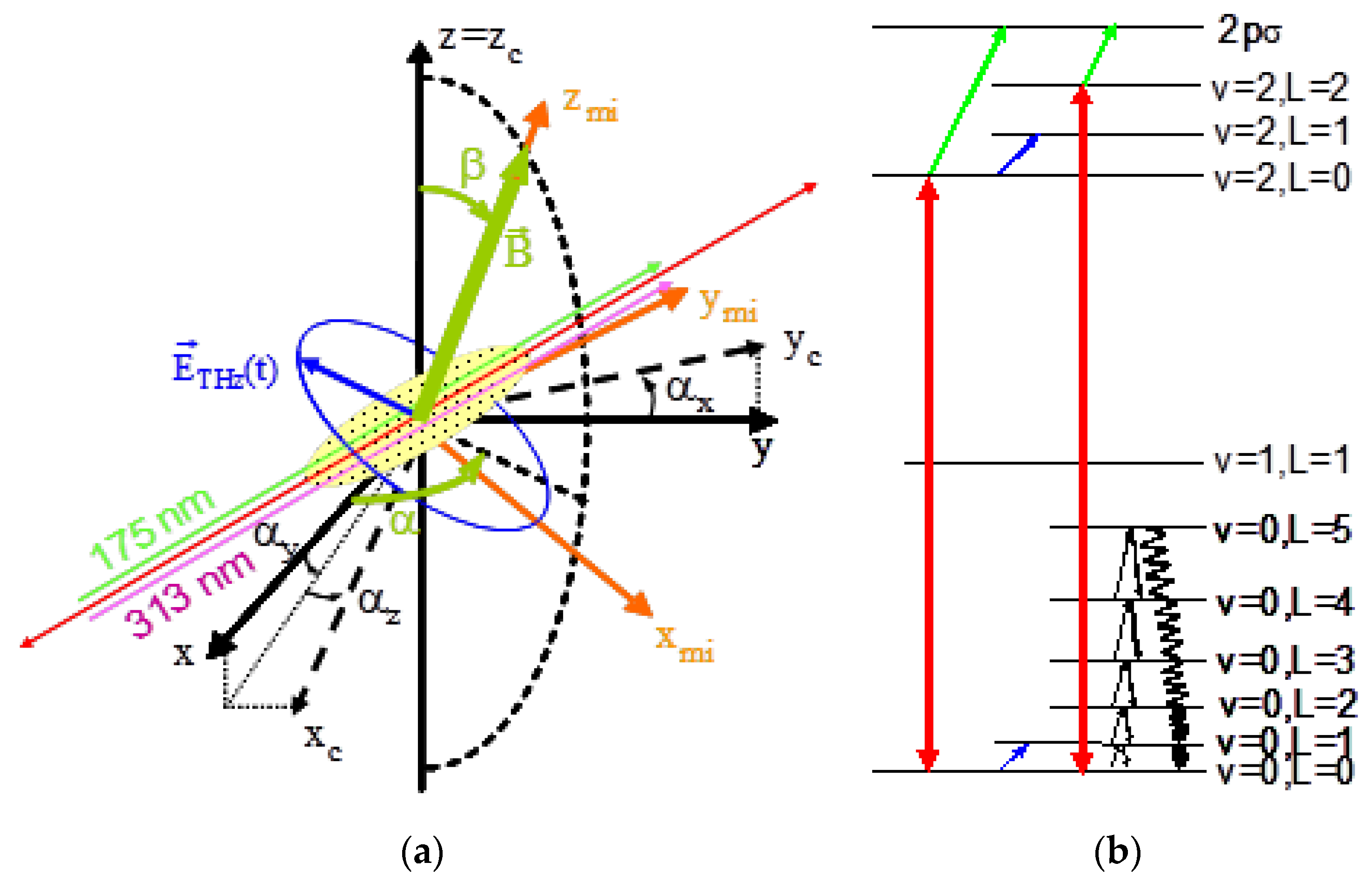
This work proposes investigating the electromagnetic fields by Doppler-free spectroscopy of the HD+ ions in a radiofrequency trap that allows narrow linewidths and small systematic shifts. The parameters characterizing the electromagnetic fields are assumed with no time dependence during the experimental measurements. The proposed experimental setup (Figure 1a) builds on previous approaches demonstrated for HD+ spectroscopy [36,38]. Typically, ≈102 HD+ ions are stored together with ≈103 Be+ ions that are laser-cooled with a 313 nm continuous-wave laser. The electrostatic interactions embed both ion species in a Coulomb crystal and sympathetically cool the HD+ ion motional degrees of freedom at the 10 mK level. The number of the HD+ ions is monitored through the change of the fluorescence of the Be+ ions at 313 nm upon excitation of the secular motion of the HD+ ions in the trap. A small static magnetic field with no spatial gradient, generated with three coil pairs in the Helmholtz configuration driven independently with three current sources, is applied to the ion trap.
Figure 1b indicates the rotation–vibration HD+ energy levels addressed in the sensing scheme. Two-photon spectroscopy is performed on the rovibrational transition (v, L) = (0, 0)→(2, 0) of HD+ using a stationary wave from an infrared laser tuned around 55.909 THz. The laser source for two-photon spectroscopy should have an ultranarrow linewidth, be tunable, and be continuously monitored against a frequency standard. These requirements may be met, for example, using the linewidth transfer technique approach [43], with a stabilized frequency comb and frequency down-conversion from near-infrared to the 5 µm spectral region. A feasible detection method is to dissociate the population transferred to the (v, L) = (2, 0) level with a 175 nm laser, as it was discussed in [44], without probing additionally a rotational transition. The population of the HD+ ions is initially distributed among the rotational levels of the ground vibrational state with a dependence determined by the thermal equilibrium with the blackbody radiation at room temperature. The blackbody radiation continuously recycles the HD+ ions population among these levels by driving electric dipole transitions, which are quantified here with the appropriate Einstein rate coefficients for spontaneous emission as well as stimulated absorption and emission. A set of rate equations, describing all transitions driven by the lasers and the blackbody radiation and taking into account the natural lifetimes of the relevant HD+ energy levels, allows characterizing the time dependence of the HD+ ions population during the resonance-enhanced multiphoton dissociation (REMPD) detection scheme assuming the hyperfine-free approximation. The lineshape of the two-photon resonance, probed with a 5362 nm laser, displays a full-width at half-maximum linewidth of 20 Hz for a two-photon transition rate of 10 s−1, a dissociation rate of 200 s−1, and an REMPD time of 10 s [44]. A similar approach based on REMPD allowed recently demonstrating the two-photon infrared spectroscopy of the (v, L) = (0, 3)→(9, 3) transition of HD+ [38]. The REMPD detection scheme proposed here estimates that a single datapoint may be recorded in 30 s, and the two-photon rovibrational line of HD+, which is used as frequency reference, may be defined within ten minutes. These timescales are comparable with the timescales of the recording of the rotational lines [37]. It is assumed that the laser can be referenced to the HD+ line with an uncertainty at a fraction of its linewidth within a ten-minute timescale.
The transitions between the spin states with a maximum total angular momentum J and extreme values of the projection Jz = ±J (stretched states) of the levels (v, L) = (0, 0) and (v, L) = (2, 0) are weakly split by the magnetic field [42]. The lightshifts of these transitions are used as probes for THz electric fields coupled off-resonantly to Zeeman subcomponents of the rotational transition (v, L) = (0, 0)→(0, 1) at 1.315 THz or (v, L) = (2, 0)→(2, 1) at 1.197 THz, respectively. The electric quadrupole shifts of the sublevels of the L = 0 states, induced by couplings with other L = 0 sublevels driven by a THz electric field with a spatial gradient, vanish [45]. The electric quadruple shifts of the sublevels of the L = 0 states due to off-resonant couplings to sublevels of the L = 2 states are neglected. In addition, the same experimental approach based on two-photon rovibrational spectroscopy of HD+ may be exploited for characterization of the magnetic field in the ion trap. Precision Zeeman spectroscopy with a 5196 nm laser of a sensitive subcomponent of the (v, L) = (0, 0)→(2, 2) two-photon transition, using a detection based on the dissociation of the (v, L) = (2, 2) level, may be exploited for determination of the magnitude of the magnetic field.
The fractional uncertainty of the frequency measurement of a transition is estimated with the Allan variance for the quantum projection noise limit:
which is expressed with the quality factor of the two-photon transition Q = f2ph/ΔfHWHM in terms of the half-linewidth ΔfHWHM. A single measurement with Nion ions at the two-photon resonance is performed during the cycle time Tc. The measurements are averaged during the interrogation time τ. For a single ion spectroscopy experiment with Tc = τ, where the linewidth is the inverse of the radiative lifetime of the excited energy level [46], the frequency uncertainty for (v, L) = (0, 0)→(2, 0) line is estimated at 2.49 Hz and for (v, L) = (0, 0)→(2, 2) line at 2.57 Hz.
This proposal is based on precision spectroscopy in an ion trap, frequency control of the spectroscopy laser, and measurements against a frequency standard, which are approaches that were previously developed for atomic ion clocks in frequency metrology institutes. The setup is a tabletop experiment involving specific lasers and optical components. Particularly, ultrastable near-infrared lasers and a stabilized frequency comb, referenced to a frequency standard, may be down-converted to the 5 µm spectral region and then amplified for two-photon spectroscopy or exploited with an enhancement cavity. The laser radiation at 175 nm may be obtained by frequency quadrupling with nonlinear crystals from a 700 nm amplified laser system.
2.3. Coordinate Frames and External Fields
The coordinate frames used here are represented in Figure 1a. The external fields applied to the HD+ ions are characterized relative to a Cartesian Laboratory Coordinate Frame locally fixed to the Earth’s surface , and its axes are pointing to East–North–Up. The Z-axis is oriented along the Earth’s ellipsoid normal direction. The magnetic field in the experimental setup is controlled with three pairs of magnetic coils. Each pair of opposite coils is driven with the same current. The coil pairs, driven independently by three stabilized current sources, define the Coil Coordinate Frame , which is not necessarily orthogonal. The orientations of the CCF axes relative to the LCF are defined with the Euler angles: for , for , and for , respectively. The nonorthogonality of the CCF axes is accounted here relative to the LCF frame with three small angles . The magnetic field vector generated by the coil pairs is expressed as:
as a function of the current-to-field parameters kx,y,z, and the coil currents I1,2,3. The conversion between the components of a vector in the orthogonal and nonorthogonal frames can be performed using a linear transformation [47].
The THz electric field vector, expressed with the complex amplitude , complex polarization vector , and angular frequency , is decomposed further in three orthogonal linearly polarized components, which read:
as a function of real positive amplitudes and phases . This dependence is represented by the polarization ellipse of the THz wave, in terms of three field amplitudes and two phases, in which the third phase is arbitrarily fixed to zero . To describe the interaction with the radiation, it is suitable to define the Cartesian Molecular Ion Coordinate Frame such that the direction of is along the direction of the magnetic field that defines the quantization axis. The THz electric field vector is expressed in the MICF using the standard components:
with real positive amplitudes and phases having linear or circular polarizations defined with . The orientation of the MICF relative to the can be changed by varying the currents in the coils. The relative orientation of the two coordinate frames is defined with the Euler angles (the third angle being fixed here arbitrarily to zero). Each standard component of the THz electric field in the MICF, denoted with , couples off-resonantly to the π or σ± Zeeman subcomponents of the (v, L) = (v, 0)→(v, 1) transitions and induces a lightshift in proportion with its squared amplitude. The standard components of the THz electric field in the MICF are related to the polarization ellipse parameters in the LCF:
2.4. Lightshifts in HD+ Spectroscopy
The coupling between the HD+ energy levels and the THz electric field is expressed in the electric dipole approximation with the interaction Hamiltonian:
where is the electric dipole operator in the laboratory frame. When the THz electric field is far from the resonance with another energy level, the lightshift of an energy level, calculated with the second-order perturbation theory [48], reads:
in terms of the matrix elements of the dipole operator, the unperturbed energy levels Er, En, and their decay rates . The matrix elements of the dipole operator have been calculated ab initio in the Born–Oppenheimer approximation using nonrelativistic three-body wavefunctions [40]. The lightshift can be related to the reduced matrix elements of the dipole operator between rovibrational states, using the tensor formalism applied to the cyclic components dq of the dipole operator. Equation (8) can be expanded with the squared modules of the standard components of the THz electric field:
The last line of Equation (9) introduces the standard dynamic polarizabilities of the HD+ energy levels ; these are expressed in terms of the complex operator , which is defined as and , having the eigenvalues .
The standard dynamic polarizabilities of the Zeeman sublevels of the (v, L) = (0, 0) and (v, L) = (2, 0) states, depending on
are calculated approximately with Equation (9), by summing over the allowed electric dipole couplings to the sublevels of the (v, L) = (0, 1) and (v, L) = (2, 1) states, respectively. The standard dynamic polarizability is a function of a set of five types of theoretical parameters—the rovibrational energies (2 parameters from [49]), the hyperfine energies (up to 11 parameters from [41]), the Zeeman energies calculated approximately with quadratic magnetic field dependences with the parameters Zk = 1,2,3 (up to 33 parameters from [42]) and Jz, the reduced dipole moment (1 parameter from [40]), the natural linewidths of the energy levels (2 parameters from [46])—and a set of experimental parameters: the magnitude of the magnetic field B, the polarization q, and the frequency of the THz wave fTHz.
In order to avoid divergences and to maintain the approximation of a far-detuned THz electric field, the contribution of the resonant coupling was neglected on a small frequency domain centered on each resonance (assumed at 10 Hz for the polarizabilities of the (v, L) = (0, 0) sublevels, and at 1.1 kHz for the polarizabilities of the (v, L) = (2, 0) sublevels, respectively).
The covariances between the differential standard dynamic polarizabilities are calculated on the basis of the analytical dependences from Equation (10) by using the error propagation law, the uncertainties of the theoretical and experimental parameters, and their correlation coefficients. The uncertainties of the theoretical rovibrational energies are estimated at a fraction of their predicted values [49]. The uncertainty of the theoretical hyperfine energies from [41] is assumed at . The uncertainty of the theoretical Zeeman parameters from [42] is assumed at . The uncertainty of the theoretical dipole moments from [40] is assumed at . The uncertainties of the theoretical radiative linewidths of the energy levels are estimated at and , by using values of energy level lifetimes from [46]. In addition, the correlation coefficients between these parameters are assumed to be equal to 1. The uncertainty of the magnitude of the magnetic field is calculated with the error propagation law by exploiting its dependence on the theoretical parameters and on the Zeeman-shifted molecular ion frequency (the approach is presented in Section 3.1). Finally, the uncertainty of the THz wave frequency is assumed at a fraction of the experimental value.
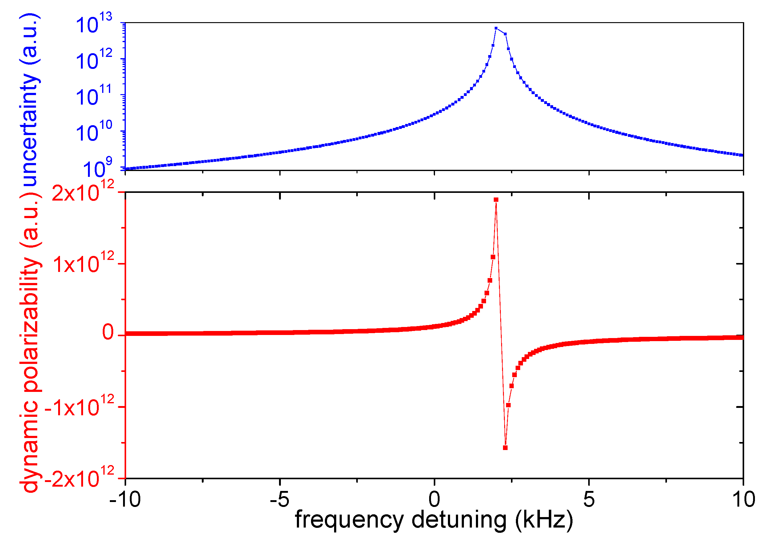
The standard dynamic polarizability of a stretched state of the ground rotational level and its uncertainty are calculated here for a given magnetic field as a function of the THz wave frequency and plotted in Figure 2. The profile of the standard dynamic polarizability has a narrow resonance when the THz wave is resonant with the transition (v, L, F, S, J, Jz) = (0, 0, 1, 2, 2, 2)→(0, 1, 1, 2, 3, 3). The uncertainty increases dramatically at resonance. Using a small detuning to the resonance for sensing a THz wave enhances the sensitivity at the expense of a loss in the calibration accuracy.
3. Results
3.1. Determination of the Magnetic Field Vector
The magnitude of the magnetic field in the ion trap can be determined from the measurements of the Zeeman shift of a two-photon rovibrational transition (v, L, F, S, J, Jz) = (n, Jz)→(n’, J’z) of HD+ by adopting the linear approximation:
as a function of the experimental frequency that is shifted by the magnetic field from the theoretical zero-field hyperfine frequency. The linear Zeeman coefficient of the two-photon transition is expressed on the second line as a function of the theoretical parameters for the Zeeman effect [42].
The magnetic field vector is controlled with three currents that drive the coil pairs independently. The uncertainty of the current in a coil pair is assumed at a fraction of the setting value. The magnetic field vector is fully described with a set of nine experimental parameters: the current-to-field parameters the nonorthogonality angles of the CCF, and the external bias magnetic field components . As a function of these parameters, the magnetic field components in the LCF read:
The set of experimental parameters can be calibrated by inversing Equation (11) using a nonlinear least-squares minimization. A number of N > 9 Zeeman spectroscopy measurements provide the Zeeman-shifted frequencies at different current setpoints . The uncertainty of the calibration procedure is evaluated with the 9 × 9 covariance matrix of the estimation errors of the model parameters:
which is expressed as a function of the N × N covariance matrix of the input data and the N × 9 Jacobian matrix , which is calculated for the input data with the assumed values of the model parameters. The value of the theoretical frequency at zero-magnetic field is expressed as the sum of the rovibrational frequency and the hyperfine frequency. The errors of the input data are estimated as the quadratic sum of the contributions from the experimental uncertainty of the Zeeman subcomponent and from the theoretical uncertainties of the rovibrational frequency the hyperfine frequency and the Zeeman shift coefficient . Nondiagonal elements in the covariance matrix of the input data arise from covariances between the theoretical parameters. The matrix reads:
Let us consider an experiment designed with the following current-to-field parameters which is operated under the Earth’s magnetic field with components along the directions east north and up with the nonorthogonality angles of the CCF assumed as The calibration is performed by Zeeman spectroscopy of the transition (v, L, F, S, J, Jz) = (0, 0, 1, 2, 2, −2)→(2, 2, 1, 2, 4, 0) of HD+. The frequencies of this Zeeman subcomponent are measured for 27 sets of current intensities = , where I0 = 1 A, Ioff1 = 3.82 mA, Ioff2 = 208 mA, Ioff3 = 422 mA, and n1,2,3 = 0,1,2. These frequency-standard calibrated measurements may be performed during a timespan estimated by five hours. The errors of the calibrated parameters , determined from the nonlinear adjustment of the Zeeman spectroscopy data, are estimated by the covariance matrix calculated using Equations (11)–(14). Particularly, the estimations for the uncertainties are:
The Cartesian components of the magnetic field in the LCF or, alternatively, the components in spherical coordinates may subsequently be derived on the basis of Equation (12), using the calibrated parameters and the currents in the coil pairs. The angular components of the magnetic field define the Euler angles in the LCF for the direction of the quantization axis. The errors for these quantities are estimated with the covariances evaluated using the error propagation law:
The previous equation expresses the covariance as the sum of the contributions from the experimental parameters determined with the magnetic field calibration procedure and from setting currents in the coil pairs.
The Earth’s magnetic field may be cancelled in the ion trap by setting the current intensities that yield a null result in Equation (12): Inull1 = −6.34 mA, Inull2 = 230 mA, and Inull3 = 434 mA. The uncertainty is estimated at 85 nT, with the root sum of squares of the uncertainties of the Cartesian components of the magnetic field in the LCF. The contribution of the Earth’s magnetic field to the total magnetic field components in the LCF is canceled when the total current in each coil pair is expressed as the sum of the nulling current with an offset current. The total currents read = in Cartesian coordinate parametrization and in spherical coordinate parametrization, respectively.
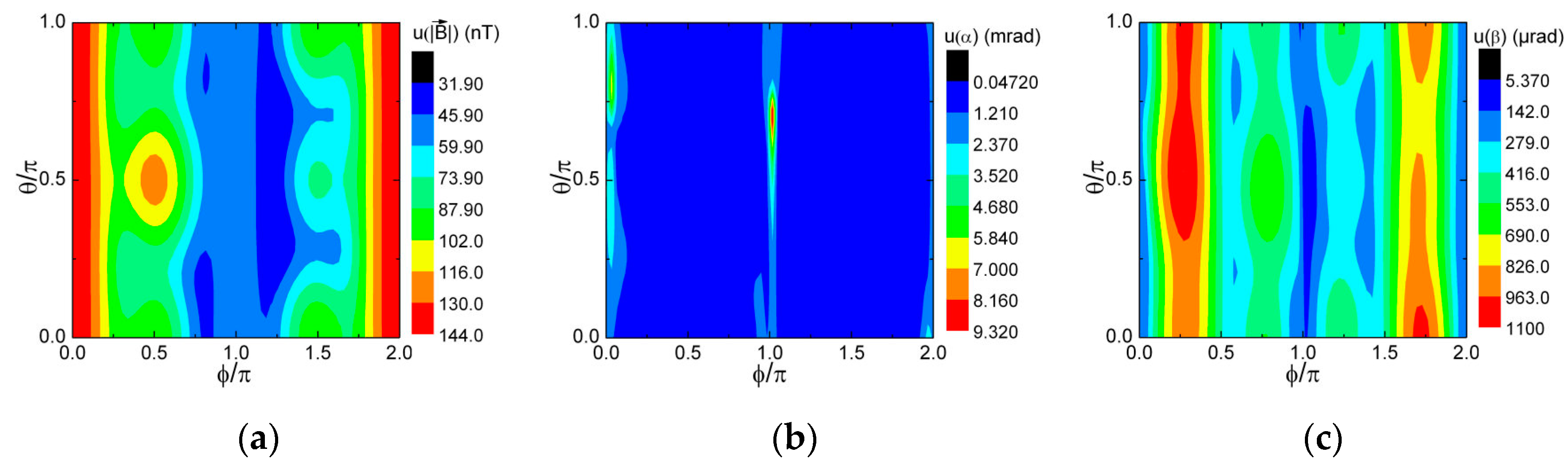
The total uncertainties of the spherical components of the magnetic field in the LCF are calculated using Equations (12)–(16) and shown in Figure 3, in the case where the total currents in the coil pairs are described by the spherical coordinate parametrization with I0 = 1 A. The uncertainties from the driving currents yield the dominant contribution to the uncertainty of the magnetic field components that is at the level or better. The contribution to this uncertainty coming only from the experimental measurements, which is at the level, is orders of magnitude smaller. Although the Euler angles do not depend on the value of the parameter I0, their uncertainties do. As for the magnitude of the magnetic field, these uncertainties decrease by increasing the value of I0.
3.2. Determination of the Polarization Ellipse of the THz Wave
The lightshifts induced on a two-photon rovibrational transition of HD+ by coupling the THz wave to the molecular ions are exploited here for characterization of the THz wave. For a given orientation of the magnetic field, three independent lightshift measurements may allow the determination of the squared modules of the standard components of the THz electric field in the MICF by solving a system of three equations depending on differential standard dynamic polarizabilities. The measurements should be performed with nondegenerate transitions that are experimentally resolved. In order to determine the amplitudes and phases of the THz electric field components in the LCF, a set of five independent measurements of the squared modules of the standard components of the electric field in the MICF are required for the inversion of Equation (6), using at least two different orientations of the magnetic field. The independence of the measurements means that the relevant systems of equations should be nonsingular. On one hand, that is possible by using different magnitudes of the magnetic field or by probing lightshifts on different two-photon hyperfine or Zeeman transitions; on the other hand, that is possible by using a set of suitable orientations of the magnetic field that takes into account the periodicity of the trigonometric functions in Equation (6). The contributions from offset THz electric fields in the LCF, similar to the blackbody radiation field, are not addressed here, and it is assumed that these fields do not vary when the THz wave is coupled to the molecular ions.
The lightshift measurements are performed by adjusting the magnitude of the magnetic field so that the THz wave is near resonant with a Zeeman subcomponent of the (v, L) = (v, 0)→(v, 1) dipole-allowed transitions of HD+. These resonance frequencies may be tuned up to ±7 GHz by applying a magnetic field up to 10−4 T. Using a small detuning to the resonance frequency is interesting for increasing the lightshift. The drawbacks are significant mixings of the Zeeman energy levels that may invalidate the second-order perturbation theory approach, a change of their populations by driving rotational transitions with the THz electric field, and a change of the quantization axis relative to the magnetic field orientation.
This work proposes exploiting six independent lightshift measurements performed on a set of two-photon transitions:
by setting suitable currents in the coil pairs such as for i = 1, 2, 3 and for i = 4, 5, 6. These measurements may be performed during a timespan by two hours. These lightshifts are related to the squared modules of the standard components of the THz electric field, which are expressed as by using the corresponding differential standard dynamic polarizabilities for the two-photon transitions. These are calculated as a function of the relevant set of theoretical parameters , the magnitude of the magnetic field expressed with the experimental parameters {Vk} that was calibrated previously by Zeeman spectroscopy, and the frequency of the THz wave. Equation (17) can be written in the matrix form by introducing a 6 × 6 matrix , which is composed of two 3 × 3 diagonal blocks having as matrix elements the differential standard dynamic polarizabilities multiplied with the suitable prefactors. The standard components of the THz electric field are derived by inversion , and their covariances are estimated from the covariances of the inverse matrix elements and the covariances of :
The errors of are assumed to be uncorrelated, and the uncertainties are the same. The second line of Equation (18) indicates the expression of the covariance of the inverse matrix elements calculated with the approach presented in [50]. The last two lines give the expression of the covariance between the differential standard dynamic polarizabilities, which are determined with the error propagation law from the covariances between the theoretical parameters , the dependences on the magnetic field magnitude, and the frequency of the THz wave, respectively. The covariances of are indicated in Section 2.4, the covariance of the magnetic field magnitudes may be calculated with Equation (16), and the uncertainty of the THz wave frequency is assumed fractionally at the ppt level.
Furthermore, the amplitudes and phases of the THz electric field components in the LCF are derived from these standard components by inverting the nonlinear system of equations of Equation (6). The solutions are expressed with the analytic dependences on for this particular choice of orientations:
In order to estimate the uncertainties, Equation (6) is linearized around these solutions:
The second line expresses the linear dependence in a compact form with the 6 × 6 Jacobian matrix , which is calculated using the solution . The errors for the amplitudes and phases of the electric field components in the LCF are given by the 5 × 5 covariance matrix of the estimation errors of the model parameters:
as a function of the 6 × 6 covariance matrix of the standard components at and , which is calculated using Equation (18).
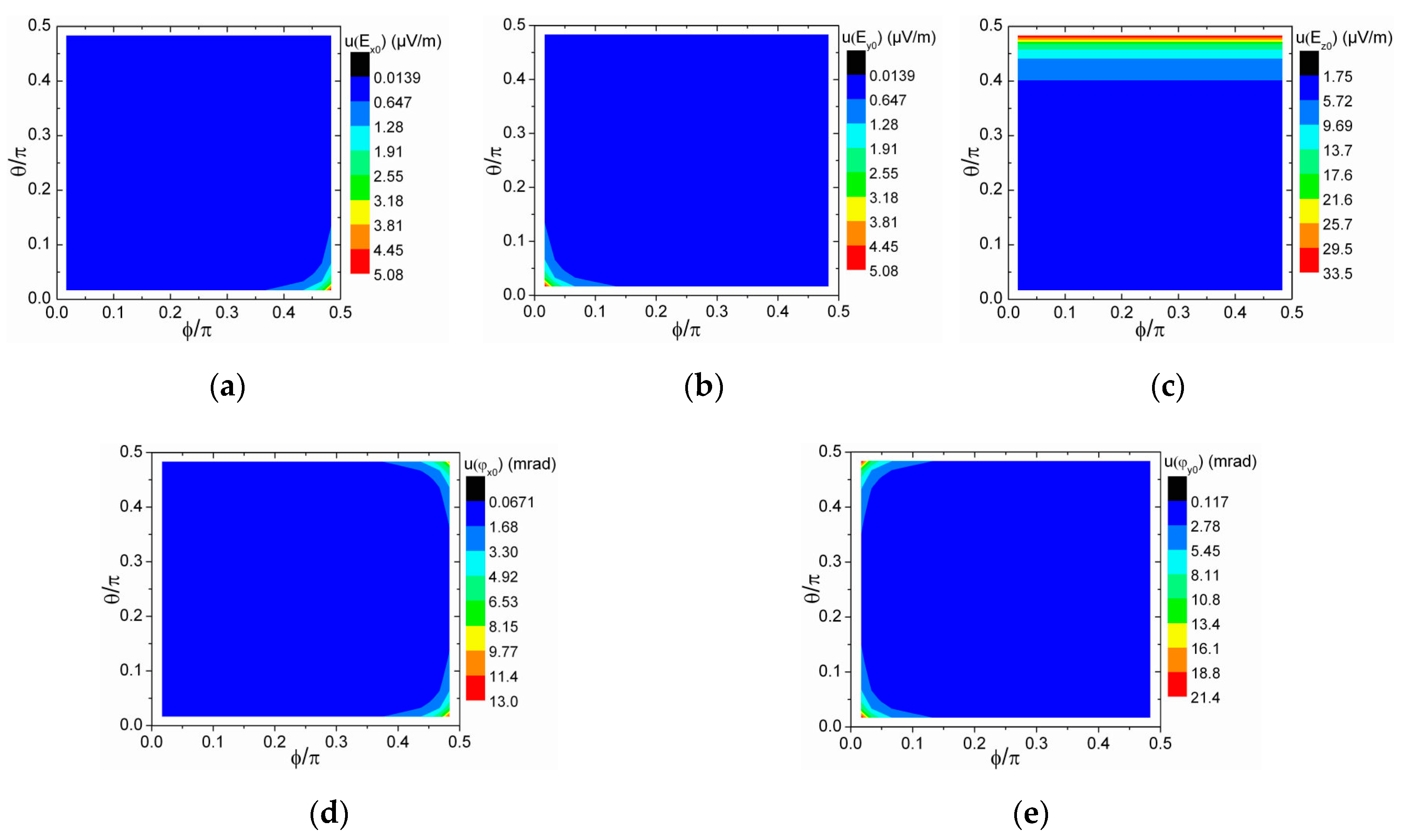
Let us discuss the application of this method for the characterization of a THz wave that is linearly polarized along an arbitrary direction. The amplitudes of the Cartesian components of the electric field are parametrized in the LCF as , as a function of the amplitude of the THz wave and two spherical angles . The relevant phases are assumed as . Here, the frequency of the THz wave is assumed at fTHz = 1,314,947,502.3 kHz (a detuning of 1.6 MHz to the frequency of the (v, L, F, S, J) = (0, 0, 1, 2, 2)→(0, 1, 1, 2, 3) hyperfine transition at zero-magnetic field) and the intensity at 1 W/m2 (E0 = 27.42 mV/m). A set of six lightshifts are measured for the two-photon transition between the stretched states (v, L, F, S, J, Jz) = (0, 0, 1, 2, 2, 2)→(2, 0, 1, 2, 2, 2) of HD+ for two orientations of the magnetic field in the case of three different values of the magnitude of the magnetic field B1 = 10−6 T, B2 = 5 × 10⁻⁶ T, and B3 = 10−5 T. The total uncertainties of the Cartesian components of the THz wave in the LCF and of their phases are calculated using Equations (16)–(21) on the basis of the standard dynamic polarizabilities given by Equation (10) and by using the calculated covariance matrix of the magnetic field components derived from Equations (11)–(14). The results are plotted in Figure 4 using the spherical angle parametrization for i = 0–30, j = 0–30. The total uncertainties are estimated at:
for a broad range of angular parameters. The uncertainty of the polarization orientation may be conservatively estimated by assuming that the total electric field uncertainty is perpendicular to the electric field direction. Summing quadratically the uncertainties of the amplitudes of the Cartesian components from Equation (22) and dividing to the amplitude yields an angular uncertainty of 2.1 × 10⁻⁴ rad.
The THz electric field parameters cannot be determined for the following sets of angular parameters because of exceedingly high uncertainties. In this case, the THz electric field may be properly characterized by using a different set of orientations of the magnetic field. The lowest uncertainties of the parameters are reached for different orientations of the polarization of the THz wave: for for for for and for That points at the importance of the choice of the orientation of the magnetic field respective to the polarization of the THz wave and to the potential accuracy with this method. Moreover, even if the uncertainties of the differential standard dynamic polarizabilities are assumed to be zero, the results plotted in Figure 4 remain nearly the same. Therefore, for these measurements, the uncertainty of the electric field characterization is dominated by the experimental uncertainties of the lightshift measurements.
The sensitivity of this method is estimated with the lowest amplitude of the THz wave for which the amplitudes and phases of the Cartesian components of the THz electric field can be determined with uncertainties smaller than the corresponding nominal values. The limit of vector detection of linearly polarized THz waves is estimated here at 350 µV/m, for which the parameters of the THz electric field can be characterized with uncertainties at the levels or better. The requirement for the uncertainties of the amplitudes is satisfied alone for a broad range of angular parameters. The requirement for the determination of the phases is satisfied only for narrow ranges of orientation of the THz wave polarization.
4. Discussion and Conclusions
This article proposes a new method to measure a THz electric field by using precision measurements of the lightshifts induced on Zeeman subcomponents of the two-photon rovibrational transition (v, L) = (0, 0)→(2, 0) of cold trapped HD+ ions detected by resonance-enhanced multiphoton dissociation. The fractional frequency uncertainty of the infrared transition measurements is estimated at the 10−12 level. An electric field oscillating by 1.3 THz is off-resonantly coupled to the electric-dipole allowed (v, L) = (0, 0)→(0, 1) rotational transition of HD+. The lightshifts of the magnetic subcomponents of the ground rotational level may be measured with uncertainties estimated with the molecular ion quantum projection noise limit at 3.5 Hz, using state-selective two-photon rovibrational spectroscopy. The THz electric field is calibrated by comparing the frequency measurements of the lightshifts against a frequency standard and the ab initio predictions of the molecular theory for the energy levels [39,41,42] and for the dipole moments [40]. This approach takes also into account the uncertainties from the theoretical calculations and ensures traceability to the SI units and to a set of fundamental constants, namely the Rydberg constant, the fine structure constant, the proton, deuteron, and electron masses, the proton and deuteron radii, the electric charge, the Planck constant [4], and the deuteron electric quadrupole moment [51].
The lightshift measurement allows scalar sensing of a THz wave. The extension toward polarization measurement is allowed by introducing a directional reference for the molecular ions—that is the quantization axis, which is defined with a static magnetic field. The SI traceability of the magnitude and of the orientation of the magnetic field is allowed by comparing two-photon rovibrational frequencies from Zeeman spectroscopy referenced to a frequency standard, with frequency measurement uncertainty estimated with the molecular ion quantum projection noise limit at 2.57 Hz, with the theoretical predictions for the HD+ energy levels. The comparison of theory and spectroscopy results based on the (v, L, F, S, J, Jz)=(0, 0, 1, 2, 2, −2)→(2, 2, 1, 2, 4, 0) transition allows the calibration of the magnetic field magnitude with an accuracy at the 10−7 T level, and it also allows defining the quantization axis with an angular accuracy at the mrad level.
The electric field of a THz wave can be fully characterized using the response of the HD+ molecular ions with respect to the quantization axis direction. The lightshift, depending on the standard components of the THz electric field, is quantified with the dynamic polarizabilities of the HD+ energy levels that are calculated here with their uncertainties. This work proposes an algorithm to calculate the values and the uncertainties of the Cartesian components of the THz electric field in the laboratory frame and their relative phases from a set of six independent lightshift measurements performed for two different orientations of the quantization axis. Although similar to the approaches demonstrated with Rabi rate measurements using coherent population transfer [52,53], this method based on lightshift measurements can allow direct referencing of the response to a frequency standard.
The application of this method to a linearly polarized THz wave with an intensity of 1 W/m2 (THz electric field amplitude 27.42 mV/m), which is detuned by 1.6 MHz from the (v, L, F, S, J) = (0, 0, 1, 2, 2)→(0, 1, 1, 2, 3) hyperfine component of the fundamental rotational transition of HD+, can allow SI calibration of the Cartesian components of the THz electric field with µV/m accuracy and of their phases with mrad accuracy for a broad range of orientations of the THz wave polarization. The accuracy of the phase measurement is two hundred times better than the previous result in microwave electric field phase measurement obtained with the Rydberg atom mixer [21]. The orientation of the polarization is determined with 0.21 mrad accuracy, which is forty times better than the vector microwave electrometry result obtained with Rydberg atom spectroscopy [20]. The lowest THz electric field vector that can be completely characterized with this method has an amplitude estimated at 350 µV/m. The detection limit in scalar THz electrometry at 11 µV/m estimated for HD+ ion spectroscopy [54] represents a 16 times improvement to the result obtained in Rydberg atom-based scalar microwave electrometry [18]. That points to the potential of lightshift measurements for THz electric field sensing—a method extensible to a number of cold trapped molecular ion species, to the optical fields, and to the magnetic components, which is compatible with the quantum enhancement techniques [32,33]. The significant improvements in performances allowed by this method compared to the traditional techniques can be of general relevance to the field of the electric field metrology.
Funding
This research received no external funding.
Conflicts of Interest
The author declares no conflict of interest.
References
- Ludlow, A.D.; Boyd, M.M.; Ye, J.; Peik, E.; Schmidt, P.O. Optical atomic clocks. Rev. Mod. Phys. 2015, 87, 637–701. [Google Scholar] [CrossRef]
- Cronin, A.D.; Schmiedmayer, J.; Pritchard, D.E. Optics and interferometry with atoms and molecules. Rev. Mod. Phys. 2009, 81, 1051–1129. [Google Scholar] [CrossRef]
- Degen, C.L.; Reinhard, F.; Cappellaro, P. Quantum sensing. Rev. Mod. Phys. 2017, 89, 035002. [Google Scholar] [CrossRef] [Green Version]
- Mohr, P.J.; Newell, D.B.; Taylor, B.N. CODATA recommended values of the fundamental physical constants: 2014. Rev. Mod. Phys. 2016, 88, 035009. [Google Scholar] [CrossRef] [Green Version]
- Sedlacek, J.A.; Schwettmann, A.; Kübler, H.; Löw, R.; Pfau, T.; Shaffer, J.P. Microwave electrometry with Rydberg atoms in a vapour cell using bright atomic resonances. Nat. Phys. 2012, 8, 819–824. [Google Scholar] [CrossRef]
- Holloway, C.L.; Gordon, J.A.; Schwarzkopf, A.; Anderson, D.A.; Miller, S.A.; Thaicharoen, N.; Raithel, G. Broadband Rydberg atom-based electric-field probe for SI traceable, self-calibrated measurements. IEEE Trans. Antenna Propag. 2014, 62, 6169–6182. [Google Scholar] [CrossRef] [Green Version]
- Camparo, J.C. Atomic stabilization of electromagnetic field strength using Rabi resonances. Phys. Rev. Lett. 1998, 80, 222–225. [Google Scholar] [CrossRef]
- Gallagher, T.F. Rydberg Atoms; Cambridge University Press: Cambridge, UK, 1994. [Google Scholar]
- Mohapatra, A.K.; Jackson, T.R.; Adams, C.S. Coherent optical detection of highly excited Rydberg states using electromagnetically induced transparency. Phys. Rev. Lett. 2007, 98, 113003. [Google Scholar] [CrossRef] [Green Version]
- Miller, S.A.; Anderson, D.A.; Raithel, G. Radio-frequency modulated Rydberg states in a vapor cell. New J. Phys. 2016, 18, 053017. [Google Scholar] [CrossRef] [Green Version]
- Gordon, J.A.; Holloway, C.L.; Schwarzkopf, A.; Anderson, D.A.; Miller, S.A.; Thaicharoen, N.; Raithel, G. Millimeter wave detection via Autler-Townes splitting in rubidium Rydberg atoms. Appl. Phys. Lett. 2014, 105, 024104. [Google Scholar] [CrossRef] [Green Version]
- Kanda, M.; Driver, L. An isotropic electric-field probe with tapered resistive dipoles for broad-band use, 100 kHz to 18 GHz. IEEE Trans. Microw. Theory Tech. 1987, 35, 124–130. [Google Scholar] [CrossRef] [Green Version]
- Hill, D.A.; Kanda, M.; Larsen, E.B.; Koepke, G.H.; Orr, R.D. Generating Standard Reference Electromagnetic Fields in the NIST Anechoic Chamber, 0.2 to 40 GHz; NIST Tech. Note 1335; National Institute of Standards and Technology: Boulder, CO, USA, 1990.
- Anderson, D.A.; Miller, S.A.; Gordon, J.A.; Holloway, C.L.; Raithel, G. Optical measurements of strong microwave fields with Rydberg atoms in a vapor cell. Phys. Rev. Appl. 2016, 5, 034003. [Google Scholar] [CrossRef] [Green Version]
- Holloway, C.L.; Simons, M.T.; Gordon, J.A.; Dienstfrey, A.; Anderson, D.A.; Raithel, G. Electric field metrology for SI traceability: Systematic measurement uncertainties in electromagnetically induced transparency in atomic vapour. J. Appl. Phys. 2017, 121, 233106. [Google Scholar] [CrossRef] [Green Version]
- Fan, H.; Kumar, S.; Sheng, J.; Shaffer, J.P.; Holloway, C.L.; Gordon, J.A. Effect of vapor-cell geometry on Rydberg-atom-based measurements of radio-frequency electric fields. Phys. Rev. Appl. 2015, 4, 044015. [Google Scholar] [CrossRef]
- Kumar, S.; Fan, H.; Sheng, J.; Shaffer, J.P. Atom-based sensing of weak radio frequency electric fields using homodyne readout. Sci. Rep. 2017, 7, 42981. [Google Scholar] [CrossRef]
- Kumar, S.; Fan, H.; Kübler, H.; Jozani, A.; Shaffer, J.P. Rydberg-atom based radio-frequency electrometry using frequency modulation spectroscopy in room temperature vapour cells. Opt. Express 2017, 25, 8625–8637. [Google Scholar] [CrossRef] [Green Version]
- Fan, H.; Kumar, S.; Sedlacek, J.; Kübler, H.; Karimkashi, S.; Shaffer, J.P. Atom based RF electric field sensing. J. Phys. B At. Mol. Opt. Phys. 2015, 48, 202001. [Google Scholar] [CrossRef]
- Sedlacek, J.A.; Schwettmann, A.; Kübler, H.; Shaffer, J.P. Atom-based vector microwave electrometry using rubidium Rydberg atoms in a vapor cell. Phys. Rev. Lett. 2013, 111, 063001. [Google Scholar] [CrossRef] [Green Version]
- Simons, M.T.; Haddab, A.H.; Gordon, J.A.; Holloway, C.L. A Rydberg atom-based mixer: Measuring the phase of a radio frequency wave. Appl. Phys. Lett. 2019, 114, 114101. [Google Scholar] [CrossRef]
- Gordon, J.A.; Simons, M.T.; Haddab, A.H.; Holloway, C.L. Weak electric-field detection with sub-1 Hz resolution at radio frequencies using a Rydberg atom-based mixer. AIP Adv. 2019, 9, 045030. [Google Scholar] [CrossRef] [Green Version]
- Wing, W.H.; Ruff, G.A.; Lamb, W.E.; Spezeski, J.J. Observation of the infrared spectrum of the hydrogen molecular ion HD+. Phys. Rev. Lett. 1976, 36, 1488–1491. [Google Scholar] [CrossRef]
- Leach, C.A.; Moss, R.E. Spectroscopy and quantum mechanics of the hydrogen molecular cation: A test of molecular quantum mechanics. Annu. Rev. Phys. Chem. 1995, 46, 55–82. [Google Scholar] [CrossRef] [PubMed]
- Critchley, A.D.J.; Hughes, A.N.; McNab, I.R. Direct measurement of a pure rotation transition in H2+. Phys. Rev. Lett. 2001, 86, 1725–1728. [Google Scholar] [CrossRef] [PubMed]
- Osterwalder, A.; Wüest, A.; Merkt, F.; Jungen, C. High-resolution millimeter wave spectroscopy and multichannel quantum defect theory of the hyperfine structure in high Rydberg states of molecular hydrogen. J. Chem. Phys. 2004, 121, 11810–11838. [Google Scholar] [CrossRef]
- Koelemeij, J.C.J.; Roth, B.; Wicht, A.; Ernsting, I.; Schiller, S. Vibrational spectroscopy of HD+ with 2-ppb accuracy. Phys. Rev. Lett. 2007, 98, 173002. [Google Scholar] [CrossRef]
- Bressel, U.; Borodin, A.; Shen, J.; Hansen, M.; Ernsting, I.; Schiller, S. Manipulation of individual hyperfine states in cold trapped molecular ions and application to HD+ frequency metrology. Phys. Rev. Lett. 2012, 108, 183003. [Google Scholar] [CrossRef] [Green Version]
- Haase, C.; Beyer, M.; Jungen, C.; Merkt, F. The fundamental rotational interval of para-H2+ by MQDT-assisted Rydberg spectroscopy of H2. J. Chem. Phys. 2015, 142, 064310. [Google Scholar] [CrossRef] [Green Version]
- Biesheuvel, J.; Karr, J.-P.; Hilico, L.; Eikema, K.S.E.; Ubachs, W.; Koelemeij, J.C.J. Probing QED and fundamental constants through laser spectroscopy of vibrational transitions in HD+. Nat. Commun. 2016, 7, 10385. [Google Scholar] [CrossRef] [Green Version]
- Roth, B.; Koelemeij, J.; Schiller, S.; Hilico, L.; Karr, J.-P.; Korobov, V.; Bakalov, D. Precision spectroscopy of molecular hydrogen ions: Towards frequency metrology of particle masses. In Precision Physics of Simple Atoms and Molecules; Karshenboim, S.G., Ed.; Springer: Berlin, Germany, 2008; Volume 745, pp. 205–232. [Google Scholar]
- Wolf, F.; Wan, Y.; Heip, J.C.; Gebert, F.; Shi, C.; Schmidt, P.O. Non-destructive state detection for quantum logic spectroscopy of molecular ions. Nature 2016, 530, 457–460. [Google Scholar] [CrossRef] [Green Version]
- Chou, C.-W.; Kurz, C.; Hume, D.B.; Plessow, P.N.; Leibrandt, D.R.; Leibfried, D. Preparation and coherent manipulation of pure quantum states of a single molecular ion. Nature 2017, 545, 203–207. [Google Scholar] [CrossRef] [Green Version]
- Tran, V.Q.; Karr, J.-P.; Douillet, A.; Koelemeij, J.C.J.; Hilico, L. Two-photon spectroscopy of trapped HD+ ions in the Lamb-Dicke regime. Phys. Rev. A 2013, 88, 033421. [Google Scholar] [CrossRef] [Green Version]
- Constantin, F.L. THz/infrared double resonance two-photon spectroscopy of HD+ for determination of fundamental constants. Atoms 2017, 5, 38. [Google Scholar] [CrossRef] [Green Version]
- Alighanbari, S.; Hansen, M.; Korobov, V.; Schiller, S. Rotational spectroscopy of cold and trapped molecular ions in the Lamb–Dicke regime. Nat. Phys. 2018, 14, 555–559. [Google Scholar] [CrossRef] [Green Version]
- Alighanbari, S.; Giri, G.S.; Constantin, F.L.; Korobov, V.; Schiller, S. Precise test of quantum electrodynamics and determination of fundamental constants with HD+ ions. Nature 2020, 581, 152–158. [Google Scholar] [CrossRef]
- Patra, S.; Germann, M.; Karr, J.-P.; Haidar, M.; Hilico, L.; Korobov, V.I.; Cozijn, F.M.J.; Eikema, K.S.E.; Ubachs, W.; Koelemeij, J.C.J. Proton-electron mass ratio from laser spectroscopy of HD+ at the part-per-trillion level. Science 2020, 369, 1238–1241. [Google Scholar] [CrossRef]
- Korobov, V.I.; Hilico, L.; Karr, J.-P. Fundamental transitions and ionization energies of the hydrogen molecular ions with few ppt uncertainty. Phys. Rev. Lett. 2017, 118, 233001. [Google Scholar] [CrossRef] [Green Version]
- Bakalov, D.; Schiller, S. Static Stark effect in the molecular ion HD+. Hyperfine Interact. 2012, 210, 25–31. [Google Scholar] [CrossRef]
- Bakalov, D.; Korobov, V.I.; Schiller, S. High-precision calculation of the hyperfine structure of the HD+ ion. Phys. Rev. Lett. 2006, 97, 243001. [Google Scholar] [CrossRef] [Green Version]
- Bakalov, D.; Korobov, V.I.; Schiller, S. Magnetic field effects in the transitions of the HD+ molecular ion and precision spectroscopy. J. Phys. B At. Mol. Opt. Phys. 2011, 44, 025003. [Google Scholar] [CrossRef]
- Akamatsu, D.; Nakajime, Y.; Inaba, H.; Hosaka, K.; Yasuda, M.; Onae, A.; Hong, F.-L. Narrow linewidth laser system realized by linewidth transfer using a fiber based frequency comb for the magneto-optical trapping of strontium. Opt. Express 2012, 20, 16010–16016. [Google Scholar] [CrossRef]
- Constantin, F.L. Double-resonance two-photon spectroscopy of hydrogen molecular ions for improved determination of fundamental constants. IEEE Trans. Instrum. Meas. 2019, 68, 2151–2159. [Google Scholar] [CrossRef]
- Bakalov, D.; Schiller, S. The electric quadrupole moment of molecular hydrogen ions and their potential for a molecular ion clock. Appl. Phys. B 2014, 114, 213–230. [Google Scholar] [CrossRef] [Green Version]
- Amitay, Z.; Zajfman, D.; Forck, P. Rotational and vibrational lifetime of isotopically asymmetrized homonuclear diatomic molecular ions. Phys. Rev. A 1994, 50, 2304–2308. [Google Scholar] [CrossRef] [PubMed]
- Pfeifer, L. Orthogonalization of nonorthogonal vector components. In Proceedings of the IEEE Position Location and Navigation Symposium ‘Navigation into the 21st Century’, Orlando, FL, USA, 29 November–2 December 1988; pp. 553–559. [Google Scholar]
- Le Kien, F.; Schneeweiss, P.; Rauschenbeutel, A. Dynamical polarizability of atoms in arbitrary light fields: General theory and application to cesium. Eur. Phys. J. D 2013, 67, 92. [Google Scholar] [CrossRef] [Green Version]
- Moss, R.E. Calculations for vibration-rotation levels of HD+, in particular for high N. Mol. Phys. 1993, 78, 371–405. [Google Scholar] [CrossRef]
- Lefebvre, M.; Keeler, R.K.; Sobie, R.; White, J. Propagation of errors for matrix inversion. Nucl. Instrum. Methods Phys. Res. A 2000, 451, 520–528. [Google Scholar] [CrossRef] [Green Version]
- Pyykkö, P. Year-2017 nuclear quadrupole moments. Mol. Phys. 2018, 116, 1328–1338. [Google Scholar] [CrossRef] [Green Version]
- Köpsell, J.; Thiele, T.; Deiglmayr, J.; Wallraff, A.; Merkt, F. Measuring the polarization of electromagnetic fields using Rabi-rate measurements with spatial resolution: Experiment and theory. Phys. Rev. A 2017, 95, 053860. [Google Scholar] [CrossRef] [Green Version]
- Thiele, T.; Lin, Y.; Brown, M.O.; Regal, C.A. Self-calibrating vector atomic magnetometry through microwave polarization reconstruction. Phys. Rev. Lett. 2018, 121, 153202. [Google Scholar] [CrossRef] [Green Version]
- Constantin, F.L. Sensing electromagnetic fields with the ac-Stark effect in two-photon spectroscopy of cold trapped HD+. In Proceedings of the SPIE 11347, Quantum Technologies 2020, Strasbourg, France, 6–10 April 2020; Diamanti, E., Ducci, S., Treps, N., Whitlock, S., Eds.; SPIE: Bellingham, WA, USA, 2020. [Google Scholar] [CrossRef]
Figure 1.
(a) The experimental setup and the reference coordinate frames. The THz electric field (blue polarization ellipse) is off-resonantly coupled to the energy levels of the HD+ ions embedded in a Coulomb crystal (yellow). Two-photon spectroscopy is performed with a stationary wave from the IR laser (red line). Be+ ions are cooled with the 313 nm laser (magenta line). The detection is performed by dissociating HD+ ions with the 175 nm laser (green line). The static magnetic field in the ion trap (olive line) can be oriented to any direction, which is defined with the Euler angles (α, β) in the Cartesian Laboratory Coordinate Frame (x, y, z) (black lines) (LCF). The orientation of the coil pairs defines the Coil Coordinate Frame (xc, yc, zc) (dotted black lines) (CCF), with the nonorthogonality angles (αx, αy, αz) relative to the laboratory frame. The standard components of the THz wave are referenced to the Cartesian Molecular Ion Coordinate Frame (xmi,ymi,zmi) (orange lines) (MICF) and related to the laboratory frame through a z–y–z rotation with the Euler angles (α, β, χ = 0). (b) Rotation–vibration energy levels of HD+ addressed in the THz sensing scheme. The two-photon rovibrational transitions are shown with red lines with arrows, the dissociation is shown with green lines with arrows, the THz wave-driven electric dipole couplings are shown with blue lines with arrows, and the blackbody-radiation-driven transitions are shown with black lines and curves with arrows.

Figure 2.
Standard dynamic polarizability σ+ (red) and its uncertainty (blue) of the stretched state |v, L, F, S, J, Jz> = |0, 0, 1, 2, 2, 2> as a function of the frequency detuning to 1,314,945,902.3 kHz (the hyperfine resonance |v, L, F, S, J> = |0, 0, 1, 2, 2>→|0, 1, 1, 2, 3> at zero-magnetic field). Magnetic field: 10−4 T.

Figure 3.
Estimated uncertainties of the spherical components of the magnetic field in the LCF as a function of the spherical angles (φ, θ) for I0 = 1 A: (a) Uncertainty of the magnetic field strength; (b) Uncertainty of the magnetic field azimuth angle; (c) Uncertainty of the magnetic field zenith angle.

Figure 4.
Estimated uncertainties of the amplitudes and phases of the components of the THz electric field in the LCF as a function of the spherical angles (φ, θ): (a) Uncertainty of Ex,0; (b) Uncertainty of Ey,0; (c) Uncertainty of Ez,0; (d) Uncertainty of φx,0; (e) Uncertainty of φy,0.
Figure 4.
Estimated uncertainties of the amplitudes and phases of the components of the THz electric field in the LCF as a function of the spherical angles (φ, θ): (a) Uncertainty of Ex,0; (b) Uncertainty of Ey,0; (c) Uncertainty of Ez,0; (d) Uncertainty of φx,0; (e) Uncertainty of φy,0.

© 2020 by the author. Licensee MDPI, Basel, Switzerland. This article is an open access article distributed under the terms and conditions of the Creative Commons Attribution (CC BY) license (http://creativecommons.org/licenses/by/4.0/).
Share and Cite
MDPI and ACS Style
Constantin, F.L. Phase-Sensitive Vector Terahertz Electrometry from Precision Spectroscopy of Molecular Ions. Atoms 2020, 8, 70. https://0-doi-org.brum.beds.ac.uk/10.3390/atoms8040070
AMA Style
Constantin FL. Phase-Sensitive Vector Terahertz Electrometry from Precision Spectroscopy of Molecular Ions. Atoms. 2020; 8(4):70. https://0-doi-org.brum.beds.ac.uk/10.3390/atoms8040070
Chicago/Turabian StyleConstantin, Florin Lucian. 2020. "Phase-Sensitive Vector Terahertz Electrometry from Precision Spectroscopy of Molecular Ions" Atoms 8, no. 4: 70. https://0-doi-org.brum.beds.ac.uk/10.3390/atoms8040070
Note that from the first issue of 2016, this journal uses article numbers instead of page numbers. See further details here.