Casimir Force between Two Vortices in a Turbulent Bose–Einstein Condensate


1
IPFN, Instituto Superior Técnico, Universidade de Lisboa, 1049-001 Lisboa, Portugal
2
Blackett Laboratory, Physics Department, Imperial College London, Prince Consort Road, London SW7 2AZ, UK
3
Instituto de Física, Universidade de São Paulo, São Paulo, SP 05508-090, Brazil
*
Author to whom correspondence should be addressed.
Atoms 2020, 8(4), 77; https://0-doi-org.brum.beds.ac.uk/10.3390/atoms8040077
Submission received: 18 September 2020
/
Revised: 26 October 2020
/
Accepted: 27 October 2020
/
Published: 4 November 2020
(This article belongs to the Section Cold Atoms, Quantum Gases and Bose-Einstein Condensation)
Abstract
:We consider the Casimir force between two vortices due to the presence of density fluctuations induced by turbulent modes in a Bose–Einstein condensate. We discuss the cases of unbounded and finite condensates. Turbulence is described as a superposition of elementary excitations (phonons or BdG modes) in the medium. Expressions for the Casimir force between two identical vortex lines are derived, assuming that the vortices behave as point particles. Our analytical model of the Casimir force is confirmed by numerical simulations of the Gross–Pitaevskii equation, where the finite size of the vortices is retained. Our results are valid in the mean-field description of the turbulent medium. However, the Casimir force due to quantum fluctuations can also be estimated, assuming the particular case where the occupation number of the phonon modes in the condensed medium is reduced to zero and only zero-point fluctuations remain.
1. Introduction
The concept of quantum vacuum plays a central role in modern physics and the Casimir force is a direct manifestation of its properties. This force was first considered for two parallel plates located at some distance in vacuum, due to quantum fluctuations of the electromagnetic vacuum field [1,2]. It was then generalised to other configurations, such as atom-wall interactions, usually called the Casimir–Polder interaction [3], and to other vacuum states, such as the acoustic vacuum in a fluid [4,5,6] and the electrostatic wave vacuum in a plasma [7]. Of particular interest was the extension, in this last reference, to the case of a turbulent medium. Here we consider the Casimir effect in this broader sense, as the mean force associated with a large spectrum of fluctuations in a medium, but quantum vacuum fluctuations will also be considered.
The Casimir effect has been previously studied in a BEC for a variety of purposes, with a major focus on the Casimir–Polder force [8,9,10,11,12], but the mechanical coupling between a two-dimensional BEC with a graphene sheet [13], and the motion of impurity atoms in a BEC [14] were also studied. Here we introduce another configuration relevant to BECs, by considering the contribution of the Casimir force to the interaction between two vortices in a turbulent BEC. This is directly relevant to the important problem of vortex-vortex interactions [15,16,17], which has been a central issue on quantum turbulence in superfluids and condensates [18]. It should also be mentioned that vortex dynamics and their interaction with the background have been also studied in a variety of papers (see, in particular, [19] and further references in [16]).
Turbulence is an important topic in quantum fluids. It has a long tradition in superfluid Helium research [20], and has also been studied in Bose–Einstein condensates (BEC) of diluted alkali vapours [21,22]. Turbulence in a quantum fluid can be seen as a non-equilibrium state resulting from the coexistence of vortices with a broad spectrum of elementary excitations in the medium. The interaction of vortices with a broad spectrum of such fluctuations is therefore recognised as an important ingredient of BEC turbulence [23].
The Casimir force can then provide an appropriate and natural tool for the diagnosis of quantum turbulence and vortex interactions. Furthermore, vortices can easily be excited in rotating or in time-varying media, and provide a spontaneous material structure on which elementary excitations can collide. From a quantum field perspective, the turbulent modes themselves can be seen as microscopic particles acting on the macroscopic structure of the vortex lines, changing both the single vortex dynamics and the two-vortex interactions. The case of single vortex dynamics could be used as a BEC analogue of Brownian motion. However, the Casimir force is clearly distinct from the addition of two independent Brownian forces, because it is intrinsically dependent on the interaction between two nearby vortices.
In this paper, we consider the Casimir force between two vortices due to the presence of density fluctuations induced by turbulent modes in a Bose–Einstein condensate. The turbulence spectrum is described as a superposition of appropriate Bogolioubov–de Gennes (BdG) modes, which are the elementary excitations of the medium. They are a special kind of phonons, sometimes also called bogolons.
In our description, two vortices are assumed immersed in a gas of quasi-particles, phonons or bogolons. We discuss the cases of both unbounded and finite condensates. The particular case of a cylindrical BEC will be considered. We use a mean-field description, which ultimately relies on the vortex and Thomas–Fermi (TF) equilibrium solutions of the Gross–Pitaevskii (GP) equation. On a more phenomenological basis, we will also be able to discuss the case of quantum fluctuations, considered as a particular case of the turbulent fluctuations where the occupation number of the quantised BdG modes tends to zero, and only the zero-point fluctuations of the quantised field remain.
2. Theoretical Model
Our theoretical framework is the GP equation describing the evolution of the condensate wavefunction , with the slow component defining the presence of topological vortices, and the (rapidly) oscillating part describing the fluctuations from the turbulent background. Here, is the chemical potential. The slow part is determined by the time-averaged GP equation [24]
with the Hamiltonian , the confining potential, and quantifying the interaction strength, where a is the scattering length. We also have defined the average density and the turbulent density , with denoting a time average.
We shall now consider the case of a condensate containing two vortices located at positions and . In a quasi-two-dimensional sample, one can consider the vortex lines parallel to the z axis. Moreover, in the case of large distances , with the healing length, we can describe them as point particles on the plane. Here, is the asymptotic value of the condensate density, far away from the vortex lines. In this case, we can show that the interaction energy (per unit length) between the two vortices is given by—see Appendix A for details
with
and , with , the topological charge of the vortices. In the absence of turbulence, , the factor becomes equal to one, as seen from Equation (A5), and we are reduced to previously known results. This allows us to determine the additional dynamical features of the two vortices, due to the presence of a turbulent background. The previous expressions are valid for , which means that this new contribution remains small.
For convenience, let us define the potential , such that . It can then be shown that the equations of motion for the two vortices can be written in the form [25]
or, alternatively
Here, we have defined the regular force as
as well as the turbulent forces
where the gradients are taken at positions . From these expressions, we can conclude that the existence of turbulent forces breaks the symmetry of the equations of motion and introduces important qualitative changes in the motion of vortex pairs. In order to understand these changes we consider the evolution of the vector distance , which evolves according to
Here, we have introduced the Casimir force between the two vortices, as defined by
This expression indicates that significant qualitative changes in the dynamics of two interacting vortices will occur in the presence of turbulence. However, we should stress that the absolute value of the Casimir force is much smaller than the usual Magnus force between vortices, .
Let us now consider the case of two identical vortices, such that . This is the most relevant case for typical experimental conditions, a discussion on which we shall elaborate later. In the absence of turbulence, Equation (8) reduces to
The two vortices rotate around their centre-of-mass (CM), with an angular frequency equal to . When we include the turbulent background, two distinct effects appear. On the one hand, the first term in Equation (8) is modified by the factor . While the modified Magnus force keeps the inter-vortex separation nearly constant, one observes a slight change on the vortex-pair rotation frequency, which becomes slow varying in time according to as the vortex pair evolves in the medium. On the other hand, the relative distance will also vary, due to the existence of the Casimir force . Notice, however, given the definition in Equation (9), that the inter-vortex radius seems to solely depend on the local density inhomogeneities (at the vortex positions). An overall attractive or repulsive interaction arises when we consider how the presence of the vortices influences the turbulent background. Since the condensate density vanishes at the centre of the vortex core, one expects a complex structure of modes that are consistent with the condition of vanishing density at the vortex core. On the average, this will lead to a vortex repulsion, rooted in a mechanism that is analogous to the well known Casimir effect between conducting plates in vacuum, as we shall demonstrate via numerical simulations of the Gross–Pitaevskii equation. In such simulations, the finite size of the vortices will be retained, in contrast with the above simple analysis, which is based on point-like vortex structures. Such a difference is not important at long distances, such that , but will eventually become relevant at short distances. (The case of finite condensates is discussed in greater detail in Appendix B).
3. Numerical Simulations
In order to understand the influence of a turbulent background on a vortex pair, we numerically integrate the two-dimensional Gross–Pitaevskii equation using a split-step Fourier scheme [26]. The two-dimensional approximation should be accurate as long as the transverse size of the sample is much larger than its longitudinal extension, in which case the degrees of freedom across this direction are essentially frozen (these include vortex-line dynamics such as Kelvin waves).
Details of the numerical integration are given: The spatial step size is 0.2 (in units of the healing length ), with a grid of points, and an integration time step of 0.01 (in units of the healing length divided by the speed of sound, ). Here, is the Bogolioubov (or sound) speed. As previously stated, the most experimentally relevant scenario is that of two vortices of equal vorticity. In this case, the co-rotation around their centre-of-mass (CM) allows for a much longer acquisition time, essential to the investigation of slow turbulence-induced dynamical features.
In order to mimic a realistic experimental scenario, we consider a finite size system, in particular, a quasi-box trap with a radius of approximately 40 —see Figure 1. This creates a quasi-homogeneous sample, a crucial ingredient to preclude any effect arising from trap inhomogeneities. The system is initialised by placing two vortices close to each other at some predetermined distance. These are placed off the axis of the trap, to prevent any symmetry induced effect of the latter. The GP equation is initially integrated in imaginary time in order to approach the ground state solution consistent with the presence of the two vortices. We start the simulation (in real time) by shaking the external potential in order to excite a turbulent wave background. This excitation last for approximately 500 s.
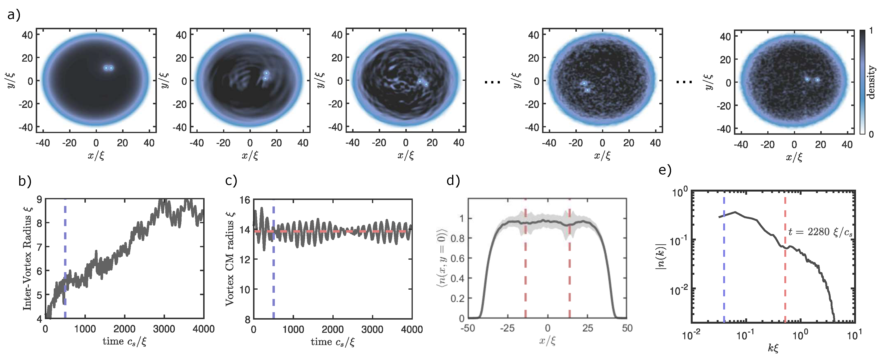
The numerical results are summarised in Figure 1. In Panels (a) and (b) we can observe a slow increase in the inter-vortex distance. The fact that the distance of the two vortices centre-of-mass to the trap axis—in Panel (c)—remains constant demonstrates that this effect originates from vortex-vortex interactions and not from trap inhomogeneities. This is also demonstrated in Panel (d), where we depict the presence of an overall homogeneous trap, at least in the regions where the vortices are present. The extent of the shaded area, indicating higher density fluctuations, is higher in the regions where the vortices travel. For illustration, we also show, in Panel (e) the power spectrum of the density fluctuations at a given instant of time.
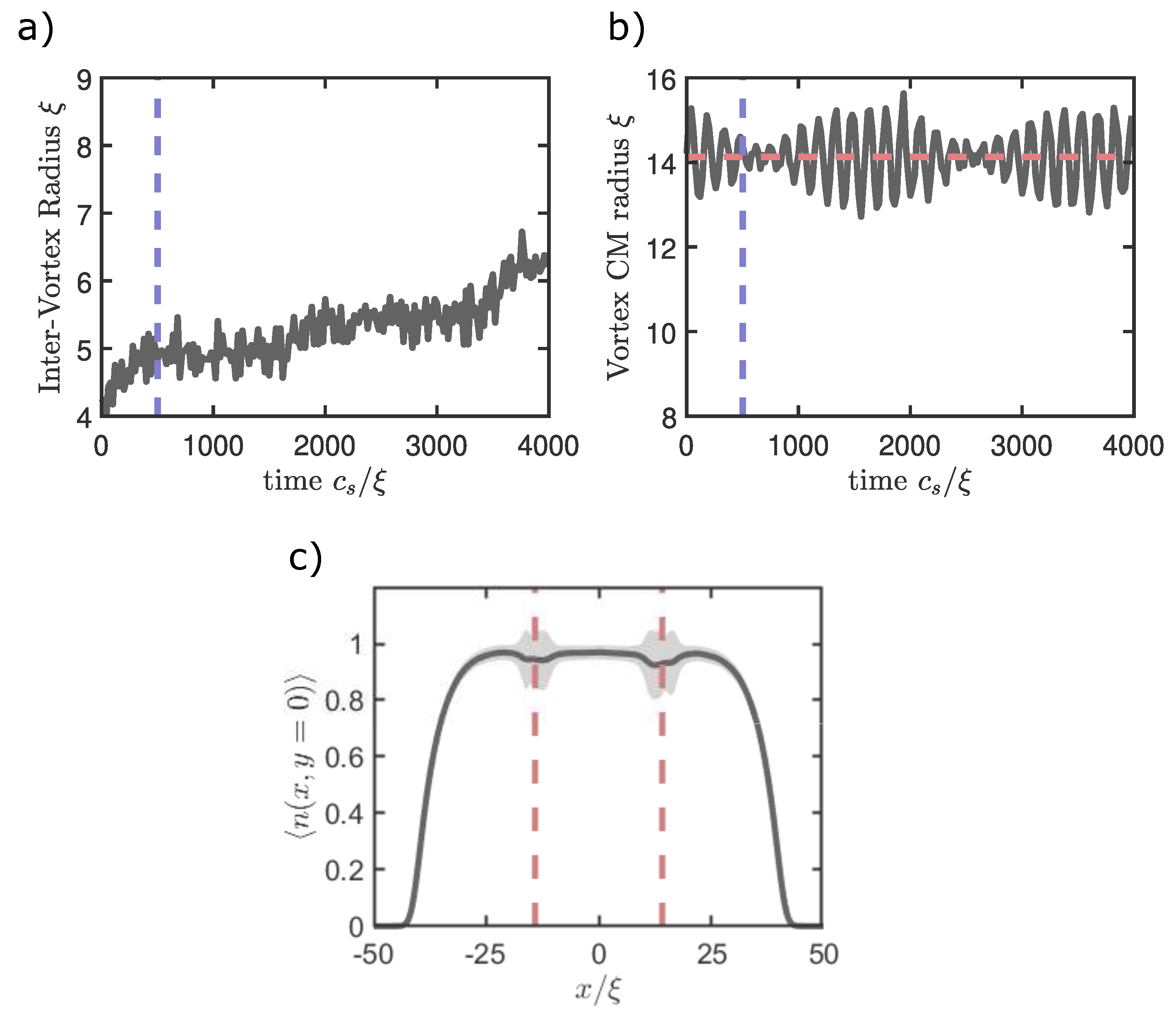
We should point out that a vortex pair, even in the presence of a quiescent background, radiates sound waves due to its co-rotational motion as well as its precession around the trap [27]. This leads to a loss of energy which, in turn, results in an increase of the inter-vortex distance. This process, however, is much slower than the effect depicted here, and is irrelevant to the present analysis. To further demonstrate this claim, we perform a simulation where all remains identical to the situation depicted in Figure 1, except that there is no initial shaking of the external potential and generation of turbulent modes is not occurring. These new simulation results are shown in Figure 2 where, in the absence of the initial shaking, we observe a much slower increase in the vortex-vortex distance. Notice, that the emission of sound waves itself induces a background of turbulent fluctuations, although of much lower amplitude, hence a much smaller effect on the vortex inter-separation. All the evidence therefore point towards the existence of vortex-vortex repulsion induced by the presence of a turbulent background.
4. Conclusions
We have studied the Casimir force between two vortices, due to vortex interactions in a turbulent medium. Both the infinite homogeneous case and the confined cylindrical configuration were considered. We have assumed that the two vortex lines were parallel to each other, but extensions of the present approach to the general case and the inclusion of Kelvin waves can also be envisaged. Our discussion was based on the well-known mean-field solutions for the average density profiles and vortex velocity profiles. The turbulent field was described as a superposition of BdG modes. The observed slow increase in the inter-vortex distance is mainly due to the unbalanced contributions of short scale and large scale oscillations to the vortex-vortex interactions, in complete analogy with the original quantum Casimir model [1,2]. We have assumed that the distance between vortices was much larger than the healing length, so that, on a plane perpendicular to the vortex lines, the two interacting vortices could be described as point particles, forming a two-dimensional dynamical system driven by the turbulent medium.
Our results show that, although the Casimir force stays much weaker that the usual mean-field force between two vortices, it introduces important qualitative changes on the dynamics of vortex pairs, which seems appropriate for experimental investigation. In particular, this force can eventually be used as an additional diagnostic of the properties of quantum turbulence. For instance, in a pair of identical vortices rotating around its centre of mass, the rotation frequency will vary in time according to the content of the turbulent spectrum, and the distance between the two vortices will not stay constant, in contrast with the case of a quiescent medium. Our analytical estimates of the turbulent Casimir force were illustrated by numerical examples and confirmed by 2D numerical simulations of the GP equation.
It would be interesting to explore the possible connection between the spacial bunching in density fluctuations with the actual value of the Casimir force. In that respect, our present numerical results are inconclusive, and a more detailed analysis is needed. We hope that the present work will stimulate theoretical and experimental work on the proposed new directions. In particular, detection of the Casimir force by measuring the distance between two nearby vortices, seems feasible using the state of the art of turbulent BEC experiments [22].
It could also be shown that our present model, although based on the mean-field approximation, is able to describe the Casimir force due to quantum zero-point fluctuations, when the occupation number of the phonon or bogolon modes in the condensed is reduced to zero. A discussion of this phenomenological approach to quantum fluctuations is included in Appendix C. A more rigorous formulation, going beyond the present mean-field approximation, will be addressed in the future.
Author Contributions
All authors contributed equally to this work. All authors have read and agreed to the published version of the manuscript.
Funding
This research was funded by the European Union Horizon 2020 program under Grant Agreement No. 820392 (PhoQuS Consortium).
Acknowledgments
J.T.M. and A.G. would like to thank the financial support of CNPq Brazil. A.G. also thanks funding of FAPESP Brazil. H.T. and J.D.R. would like to thank FCT Portugal for support.
Conflicts of Interest
The authors declare no conflict of interest.
Appendix A. Energy of Two Vortices
We consider cylindrical coordinates . Using the standard definition for the vortex energy [28,29], for a single vortex with topological charge ℓ, axis parallel to the z-direction and location at , we obtain
This is the energy per unit length, taken over a cylindrical volume with size , with the healing length . This differs from the usual expression for , by the addition of a term proportional to turbulent density . This is only valid for , which means that this new contribution remains small. However, it will introduce important qualitative changes.
Let us now consider two interacting vortices, immersed in the turbulent medium. For vortex lines parallel to the z-axis and positions in the perpendicular plane described by , with , such that , we can describe them as point particles on this plane. The total vortex energy is , where are the single vortex energies considered above, and is the interaction energy
where . The vortex velocities can be defined as
Noting that , and that the Green’s function is solution of the equation , we can obtain after integration by parts, the total energy (per unit length)
with
Here, we have symmetrised the result with respect to and .
Appendix B. The Case of Finite Condensates
Let us consider vortices in a cylindrical condensate. In the presence of turbulence, we can define a modified Thomas–Fermi (TF) equilibrium profile , with a radius , such that [24]
where refers to a quiescent medium. The energy of a single vortex located at, , is [28,29]
This differs from the usual value in the absence of turbulence, , for two reasons: first, because the radius of the condensate has changed from to a; second, because the background density has also changed, from to . We can approximately write , where is the unperturbed energy
and the additional energy associated with turbulence is determined by
Using Equation (A6), this can also be written as
It is useful to describe turbulence as a superposition of BdG modes such that [24]
where are the mode amplitudes, and the radial mode functions. Here, as the successive zeros of the Bessel functions, such that , and are normalisation factors. The mode frequency is related with the axial wavenumber through the BdG dispersion relation [24]. in general, the time average defining the turbulent density is taken over a period larger than that of the relevant BdG modes. This is compatible with the existence of very slow time variations, due to a slow beating between different modes, eventually non-negligible with respect with the rotation frequency .
If we now have two different vortices at a distance , both located at but on different angles with respect to the axis, their interaction energy (per unit length) will be
For a modified TF density profile, we can use , where is the density at the centre. Assuming the generic turbulent modes of Equation (A11), we can also write: , where the purely radial part of the turbulent density fluctuations is defined by
and the angular part results from the beating between modes with different helicity, as
where . A similar beating between modes with different axial wavenumber k could also be defined, but with no influence on the vortex interaction processes described here.
Following the same procedure as for the case of an unbounded medium, we can then derive an expression for the Casimir force, formally identical to Equation (9). For turbulence with a cylindrical symmetry and , we are reduced to
This shows that, for identical vortex numbers , located opposite to each other, the Casimir force can only result from a cylindrical symmetry breaking of the background turbulence. In the simplest case, this can result from the beating between two BdG modes with different values of , as shown by Equation (A14). For a single mode , we simply have .
Appendix C. Quantum Fluctuations
Fluctuations of the quantised turbulent vacuum become relevant when the amplitude of the turbulent modes tends to zero. Only fluctuations associated with the zero-point energy of the BdG mode spectrum will remains. In order to calculate the corresponding Casimir force, we start with the energy associated with the turbulent modes . We have previously noticed that the turbulent density can be described by mode superposition. Using Equation (A13), we can then write for a cylindrical condensate:
This should be compared with the energy associated with the mode quantisation, which can be stated as
Here, are the mode occupation numbers, defined as the expectation values of the product between the creation and destruction operators, in the usual way. For a given axial wavenumber k, the BdG mode frequencies satisfy the dispersion relation , where is the Bogolioubov sound speed [24]. Comparing the two expressions of and , for , we obtain the zero-point density fluctuations of the BdG spectrum, as
The turbulent density profile associated with these zero point fluctuations can then be determined as
Given the weak dependence of the mode frequency with respect to the helicity , we can assume that the amplitudes associated with the angular part of the fluctuations (A14) are of the same order. We should notice that the summation over the quantum modes extends to infinity, which means that appropriate cutoffs should be used. This could be determined by the relevant temporal scales the boundary conditions.
In this phenomenological model, the zero-point fluctuations are described as a limiting case of the turbulent fluctuations. The advantage of such an approach is that it provides a unifying description of both turbulence and quantum fluctuations. However, the spectral cutoffs remain uncertain and a more rigorous formulation of quantum turbulence will be needed.
References
- Casimir, H.B.G. On the attraction between two perfectly conducting plates. Proc. Kon. Ned. Akad. Wet. 1948, 51, 793. [Google Scholar]
- Milton, K.A. The Casimir Effect: Physical Manifestations of Zero-Point Energy; World Scientific: Singapore, 2011. [Google Scholar]
- Casimir, H.B.G.; Polder, D. The influence of retardation on the London-van de Waals forces. Phys. Rev. 1948, 73, 360. [Google Scholar] [CrossRef]
- Larraza, A.; Holmes, C.D.; Susbulla, R.T. The force between two parallel rigid plates due to the radiation pressure of broadband noise: An acoustic Casimir effect. J. Acoust. Soc. Am. 1998, 103, 2763. [Google Scholar] [CrossRef]
- Denardo, B.C.; Puda, J.J.; Larraza, A. A water wave analog of the Casimir effect. Am. J. Phys. 2009, 77, 1095. [Google Scholar] [CrossRef] [Green Version]
- Jaskula, J.-C.; Partridge, G.B.; Bonneau, M.; Lopes, R.; Ruaudel, J.; Boiron, D.; Westbrook, C.I. Acoustic analog of the dynamical Casimir effect in a Bose-Einstein condensate. Phys. Rev. Lett. 2012, 109, 220401. [Google Scholar] [CrossRef] [PubMed] [Green Version]
- Mendonça, J.T.; Bingham, R.; Shukla, P.K.; Resendes, D. Casimir effect in a turbulent plasma. Phys. Lett. A 2001, 289, 233. [Google Scholar] [CrossRef]
- Pasquini, T.A.; Shin, Y.; Sanner, C.; Saba, M.; Schirotzek, A.; Pritchard, D.E.; Ketterle, W. Quantum reflection from a solid surface at normal incidence. Phys. Rev. Lett. 2004, 93, 223201. [Google Scholar] [CrossRef] [PubMed] [Green Version]
- Harber, D.M.; Obrecht, J.M.; McGuirk, J.M.; Cornell, E.A. Measurement of the Casimir-Polder force through center-of-mass oscillations of a Bose-Einstein condensate. Phys. Rev. A 2005, 72, 033610. [Google Scholar] [CrossRef] [Green Version]
- Impens, F.; Contreras-Reyes, A.M.; Neto, P.A.M.; Dalvit, D.A.R.; Guérout, R.; Lambrecht, A.; Reynaud, S. Driving quantized vortices with quantum vacuum fluctuations. EuroPhys. Lett. 2010, 92, 40010. [Google Scholar] [CrossRef]
- Moreno, G.A.; Messina, R.; Dalvit, D.A.R.; Lambrecht, A.; Neto, P.A.M.; Reynaud, S. Disorder in quantum vacuum: Casimir-induced localization of matter waves. Phys. Rev. Lett. 2010, 105, 210401. [Google Scholar] [CrossRef] [Green Version]
- Bender, H.; Stehle, C.; Zimmermann, C.; Slama, S.; Fiedler, J.; Scheel, S.; Buhmann, S.Y.; Marachevsky, V.N. Probing atom-surface interactions by diffraction of Bose-Einstein condensates. Phys. Rev. X 2014, 4, 011029. [Google Scholar] [CrossRef] [Green Version]
- Terças, H.; Ribeiro, S.; Mendonça, J.T. Quasi-polaritons in Bose-Einstein condensates induced by Casimir-Polder interaction with graphene. J. Phys. Condens. Matter 2015, 27, 214011. [Google Scholar] [CrossRef] [PubMed] [Green Version]
- Marino, J.; Recati, A.; Carusotto, I. Casimir forces and quantum friction from Ginzburg radiation in atomic Bose-Einstein condensates. Phys. Rev. Lett. 2017, 118, 045401. [Google Scholar] [CrossRef] [Green Version]
- Serafini, S.; Barbiero, M.; Debrotoli, M.; Donatello, S.; Larcher, F.; Dalfovo, F.; Lamporesi, G.; Ferrari, G. Dynamics and interaction of vortex lines in an elongated Bose-Einstein condensate. Phys. Rev. Lett. 2015, 115, 170402. [Google Scholar] [CrossRef]
- Fetter, A. Rotating trapped Bose-Einstein condensates. Rev. Mod. Phys. 2009, 81, 647. [Google Scholar] [CrossRef] [Green Version]
- Sonin, E.B. Vortex oscillations and hydrodynamics of rotating superfluids. Rev. Mod. Phys. 1987, 59, 87. [Google Scholar] [CrossRef]
- Paoletti, M.S.; Lathrop, D.P. Quantum turbulence. Annu. Rev. Condens. Matter Phys. 2011, 2, 213. [Google Scholar] [CrossRef] [Green Version]
- Sheehy, D.E.; Radzihovsky, L. Vortices in spatially inhomogeneous superfluids. Phys. Rev. A 2004, 70, 063620. [Google Scholar] [CrossRef] [Green Version]
- Skrbek, L.; Sreenivasan, K.R. Developed quantum turbulence and its decay. Phys. Fluids 2012, 24, 011301. [Google Scholar] [CrossRef]
- Henn, E.A.L.; Seman, J.A.; Roati, G.; Magalhães, K.M.F.; Bagnato, V.S. Emergence of turbulence in an oscillating Bose-Einstein condensate. Phys. Rev. Lett. 2009, 103, 045301. [Google Scholar] [CrossRef] [PubMed]
- Madeira, L.; Cidrim, A.; Hemmerling, M.; Caracanhas, M.A.; dos Santos, F.E.A.; Bagnato, V.S. Quantum turbulence in Bose-Einstein condensates: Present status and new challenges ahead. AVS Quantum Sci. 2020, 2, 035901. [Google Scholar] [CrossRef]
- White, A.C.; Proukakis, N.P.; Youd, A.J.; Wacks, D.H.; Baggaley, A.W.; Barenghi, C.F. Turbulence in a Bose-Einstein condensate. J. Phys. Conf. Ser. 2011, 318, 062003. [Google Scholar] [CrossRef]
- Mendonça, J.T.; Haas, F.; Gammal, A. Nonlinear vortex-phonon interactions in a Bose-Einstein condensate. J. Phys. B At. Mol. Opt. Phys. 2016, 49, 145302. [Google Scholar] [CrossRef]
- Calderaro, L.; Fetter, A.L.; Massignan, P.; Wittek, P. Vortex dynamics in coherently coupled Bose-Einstein condensates. Phys. Rev. A 2017, 95, 023605. [Google Scholar] [CrossRef] [Green Version]
- Antoine, X.; Boa, W.; Besse, C. Computational methods for the dynamics of the nonlinear Schrödinger/Gross-Pitaevskii equations. Comp. Phys. Commun. 2013, 184, 2621. [Google Scholar] [CrossRef] [Green Version]
- Parker, N.G.; Proukakis, N.P.; Barenghi, C.F.; Adams, C.S. Controlled vortex-sound interactions in atomic Bose-Einstein condensates. Phys. Rev. Lett. 2004, 92, 160403. [Google Scholar] [CrossRef] [Green Version]
- Pethick, C.; Smith, H. Bose–Einstein Condensates in Dilute Gases; Cambridge University Press: Cambridge, UK, 2008. [Google Scholar]
- Pitaevskii, L.; Stringari, S. Landau damping in dilute Bose gases. Phys. Lett. A 1997, 235, 398. [Google Scholar] [CrossRef] [Green Version]
Figure 1.
(color online) Panel (a) depicts a typical simulation. The first three plots correspond to 0, 250, 500 , during the shaking of the external potential. The remaining density maps depict later stages, at 2000, 4000 , respectively, where vortices evolve a fully developed turbulent background. Notice that the vortex dipole precesses around the trap axis due to the total content of orbital angular momentum in the system. The inter-vortex distance and the dipole centre-of-mass distance to the trap axis is plotted in panels (b,c), respectively. Here, the vertical blue line corresponds to the end of the potential shaking step, while the red line in panel (c) depicts the average CM distance. In panel (d) we plot the density profile across a slice 0, with denoting time average (during the entire simulation span) and the red lines indicating the average CM distance, as before. Moreover, the shaded are corresponds to the one sigma level of density fluctuations. Panel (e) depicts the power spectrum of the density fluctuations for a particular time instant, with the blue and red lines indicating the scales associated with the size of the trap and mean inter-vortex radius.

Figure 2.
(color online) Simulation in the absence of potential shaking. Here Panels (a–c) are equivalent to Panels (b–d) of Figure 1.
Figure 2.
(color online) Simulation in the absence of potential shaking. Here Panels (a–c) are equivalent to Panels (b–d) of Figure 1.

Publisher’s Note: MDPI stays neutral with regard to jurisdictional claims in published maps and institutional affiliations. |
© 2020 by the authors. Licensee MDPI, Basel, Switzerland. This article is an open access article distributed under the terms and conditions of the Creative Commons Attribution (CC BY) license (http://creativecommons.org/licenses/by/4.0/).
Share and Cite
MDPI and ACS Style
Mendonça, J.T.; Terças, H.; Rodrigues, J.D.; Gammal, A. Casimir Force between Two Vortices in a Turbulent Bose–Einstein Condensate. Atoms 2020, 8, 77. https://0-doi-org.brum.beds.ac.uk/10.3390/atoms8040077
AMA Style
Mendonça JT, Terças H, Rodrigues JD, Gammal A. Casimir Force between Two Vortices in a Turbulent Bose–Einstein Condensate. Atoms. 2020; 8(4):77. https://0-doi-org.brum.beds.ac.uk/10.3390/atoms8040077
Chicago/Turabian StyleMendonça, José Tito, Hugo Terças, João D. Rodrigues, and Arnaldo Gammal. 2020. "Casimir Force between Two Vortices in a Turbulent Bose–Einstein Condensate" Atoms 8, no. 4: 77. https://0-doi-org.brum.beds.ac.uk/10.3390/atoms8040077
Note that from the first issue of 2016, this journal uses article numbers instead of page numbers. See further details here.