Scattering and Its Applications to Various Atomic Processes: Elastic Scattering, Resonances, Photoabsorption, Rydberg States, and Opacity of the Atmosphere of the Sun and Stellar Objects

Abstract
:1. Introduction
2. Calculations Involving Electrons
3. Hybrid Theory
4. Photoabsorption
5. Recombination Rates
6. Photoejection with Excitation
7. Excitation by Electron Impact
8. Resonances
9. Polarizabilities
10. Optical Properties of Helium Gas
11. Lamb Shift
12. Retardation Correction (Casimir)
13. Hyperfine Structure of Li
14. Parity-Violating Electric-Dipole Transitions in Helium
15. Positron–Hydrogen Scattering
16. Zeff
17. Positronium Formation
18. Resonances in Systems Involving Positrons
19. Resonances in Positronium Ion
20. Positron Impact Excitation
21. High-Energy Cross-Sections
22. Photodetachment of a Positronium Ion
23. Opacity of the Atmosphere of the Sun
24. Conclusions
Funding
Conflicts of Interest
References
- Compton, A.H. A Quantum Theory of the scattering of X-rays by light. Elements. Phys. Rev. 1923, 21, 152. [Google Scholar] [CrossRef]
- Bothe, W.; Geiger, H. Uber das Wesen des Compton effects ein experimenteller Breitrag Theorie der Strahlung. Zeits für Phys. 1925, 22, 639. [Google Scholar] [CrossRef]
- Compton, A.H.; Simon, A.W. Directed Quanta of Scattered X-rays. Phys. Rev. 1925, 26, 289. [Google Scholar] [CrossRef]
- Bohr, N.; Kramers, H.A.; Slaters, J.C. The quantum theory of radiation. Phil. Mag. J. Science. 1924, 47, 785. [Google Scholar] [CrossRef]
- Schrödinger, E. An undulatory theory of the mechanics of atoms and molecules. Phys. Rev. 1926, 28, 1049. [Google Scholar] [CrossRef]
- Chadwick, J. Possible Existence of a neutron. Nature 1932, 129, 312. [Google Scholar] [CrossRef]
- Temkin, A. A note on Scattering of Electrons from Atomic Hydrogen. Phys. Rev. 1959, 116, 358. [Google Scholar] [CrossRef]
- Mittleman, M.H. Resonances in Proton-Hydrogen and Positron-Hydrogen. Phys. Rev. 1966, 152, 76. [Google Scholar] [CrossRef]
- Casimir, H.B.G.; Polder, D. The influence of Radiation on the London-van der Waals Forces. Phys. Rev. 1948, 73, 360. [Google Scholar] [CrossRef]
- Kelsey, E.J.; Spruch, L. Radiation effects on high Rydberg States. A retarded R−5polarization potential. Phys. Rev. A 1978, 18, 15. [Google Scholar] [CrossRef]
- Lundeen, S.R. Experimental Studies of High-L High Rydberg States in Helium in Long-Range Casimir Forces Theory and Experiments on Atomic Systems; Levin, F.S., Micha, D.A., Eds.; Plenum Press: New York, NY, USA, 1993; p. 73. [Google Scholar]
- Morse, P.M.; Allis, W.P. The effect of Exchange on the scattering of Slow Electrons from Atoms. Phys. Rev. 1933, 44, 269. [Google Scholar] [CrossRef]
- Sloan, I.H. The method of polarized orbitals for the elastic scattering of slow electrons by ionized helium and atomic hydrogen. Proc. Roy. Soc. 1961, 281, 151. [Google Scholar]
- Burke, P.G.; Smith, K. The Low-Energy Scattering of Electrons and Positrons by Hydrogen Atoms. Rev. Mod. Phys. 1962, 34, 458. [Google Scholar] [CrossRef]
- Burke, P.G.; Robb, W.D. The R-Matrix Theory of Atomic Processes. Adv. Atom. Mole. Phys. 1976, 11, 143. [Google Scholar]
- Burke, P.G.; Noble, C.J.; Scott, M.P. Electron-hydrogen atom scattering at intermediate energies. Proc. Roy. Soc. A 1987, 410, 289. [Google Scholar]
- Schwartz, C. Electron Scattering from hydrogen. Phys. Rev. 1961, 124, 1468. [Google Scholar] [CrossRef] [Green Version]
- Feshbach, H. A unified theory of nuclear reactions II. Ann. Phys. (NY.) 1962, 19, 287. [Google Scholar] [CrossRef]
- Bhatia, A.K.; Temkin, A. Complex-correlation Kohn T-matrix method of calculating total cross sections: Electron-hydrogen elastic scattering. Phys. Rev. A 2001, 64, 032709. [Google Scholar] [CrossRef]
- McCurdy, C.W.; Baertschy, M.; Rescigno, T.N. Solving the three-body Coulomb breakup problem. J. Phys. B 2004, 37, R137. [Google Scholar] [CrossRef]
- Bhatia, A.K. Hybrid theory of electron-hydrogen elastic scattering. Phys. Rev. A 2007, 75, 032713. [Google Scholar] [CrossRef]
- Bhatia, A.K.; Temkin, A. Symmetric Euler-Angle Decomposition of the Two-Electron Fixed-Nucleus Problem. Rev. Mod. Phys. 1964, 36, 1050. [Google Scholar] [CrossRef] [Green Version]
- Temkin, A. Polarization and the Triplet-Electron Hydrogen Scattering Length. Phys. Rev. Lett. 1961, 6, 354. [Google Scholar] [CrossRef]
- Oza, D.H. Phase shifts and resonances for electron scattering by He+ below N = 2 threshold. Phys. Rev. A 1986, 33, 824. [Google Scholar] [CrossRef]
- Bhatia, A.K. Applications of the hybrid theory to the scattering of electrons from He+ and Li2+. Phys. Rev. A 2008, 77, 052707. [Google Scholar] [CrossRef]
- Gien, T.T. Accurate calculation of phase shifts for electron-He+ collisions. J. Phys. B 2002, 35, 4475. [Google Scholar] [CrossRef]
- Gien, T.T. Accurate calculation of phase shifts for electron-Li2+ collisions. J. Phys. B 2003, 36, 2291. [Google Scholar] [CrossRef]
- Bhatia, A.K. Electron-He+ elastic Scattering. Phys. Rev. A 2002, 66, 06472. [Google Scholar] [CrossRef]
- Wildt, R. Electron Affinity in Astrophysics. Astrophys. J. 1939, 89, 295. [Google Scholar] [CrossRef]
- Chandrasekhar, S. On the Continuous Absorption Coefficient of the negative Hydrogen Ion. Astrophys. J. 1945, 102, 223. [Google Scholar] [CrossRef]
- Bhatia, A.K. Electron-He+ P-wave elastic scattering and photoabsorption in two-electron systems. Phys. Rev. A 2006, 73, 012705. [Google Scholar] [CrossRef]
- Bhatia, A.K. Hybrid theory of P-wave electron-Li2+elastic scattering and photoabsorption in two electron systems. Phys. Rev. A 2013, 87, 042705. [Google Scholar] [CrossRef]
- Wishart, A.W. The bound—free photodetachment of H. J. Phys. B 1979, 12, 3511. [Google Scholar] [CrossRef]
- Branscomb, L.M.; Smith, S.J. Experimental Cross Sections for Photodetachment of Electrons from H- and D. Phys. Rev. 1955, 98, 1028. [Google Scholar] [CrossRef]
- Ohmura, T.; Ohmura, H. Electron-Hydrogen scattering at low energies. Phys. Rev. 1960, 118, 154. [Google Scholar] [CrossRef]
- Nahar, S.N. The Ultraviolet Properties of Evolved Stellar Populations. In New Quests in Stellar Astrophysics II; Chavez, M., Bertone, E., Rosa-Gonzalez, D., Rodriguez-Merino, L.H., Eds.; Springer: New York, NY, USA, 2009; p. 245. [Google Scholar]
- Samson, J.A.; He, Z.X.; Yin, L.; Haddad, G.N. Precision measurements of the absolute photoionization cross sections of He. J. Phys. B 1994, 27, 887. [Google Scholar] [CrossRef]
- Daskhan, M.; Ghosh, A.S. Photoionization of He and Li+. Phys. Rev. A 1984, 86, 032713. [Google Scholar]
- Bhatia, A.K.; Temkin, A.; Silver, A. Photoionization of Li. Phys. Rev. A 1975, 12, 2044. [Google Scholar] [CrossRef]
- Dasgupta, A.; Bhatia, A.K. Photoionization of Sodium Atoms and Electron scattering from Ionized Sodium Atoms. Phys. Rev. A 1985, 31, 759. [Google Scholar] [CrossRef] [PubMed]
- Bhatia, A.K.; Drachman, R.J. Photoejection with excitation in H- and other systems. Phys. Rev. A 2015, 91, 012702. [Google Scholar] [CrossRef]
- Bhatia, A.K. Application of P-wave hybrid theory for the scattering of electrons from He+and resonances in He and H. Phys. Rev. A 2007, 86, 032713. [Google Scholar] [CrossRef]
- Callaway, J. Scattering of electrons by atomic hydrogen at intermediate energies. Elastic Scattering and n = 2 excitation from 12 to 54 eV. Phys. Rev. A 1985, 32, 775. [Google Scholar] [CrossRef]
- Burke, P.G.; Schey, H.M.; Smith, K. Collisions of slow Electrons and Positrons with Atomic Hydrogen. Phys. Rev. 1963, 129, 1258. [Google Scholar] [CrossRef] [Green Version]
- Scott, M.P.; Scholz, T.T.; Walters, H.R.; Burke, P.G. Electron scattering by atomic hydrogen at intermediate energies: Integrated elastic 1s-2s and 1s-2p cross sections. J. Phys. B 1989, 22, 3055. [Google Scholar] [CrossRef]
- Madden, R.P.; Codling, K. Two-Electron Excitation States of Helium. Ap. J. 1965, 141, 364. [Google Scholar] [CrossRef]
- Bhatia, A.K.; Burke, P.G.; Temkin, A. Calculation of (2s2p) 1P Autoionization State of He with a Pseudostate Nonresonant Continuum. Phys. Rev. A 1973, 8, 21. [Google Scholar] [CrossRef]
- Bhatia, A.K. Autoionization and quasibound states of Li+. Phys. Rev. A 1977, 15, 1315. [Google Scholar] [CrossRef]
- Drake, G.W.F. High-Precision Calculations for The Rydberg States of Helium in Long-Range Casimir Forces Theory and Experiments on Atomic Systems; Levin, F.S., Micha, D.A., Eds.; Plenum Press: New York, NY, USA, 1993; p. 107. [Google Scholar]
- Drachman, R.J. High Rydberg States of Two-Electron Atoms in Perturbation Theory in Long-Range Casimir Forces Theory and Experiments on Atomic Systems; Levin, F.S., Micha, D.A., Eds.; Plenum Press: New York, NY, USA, 1993; p. 219. [Google Scholar]
- Rothery, N.E.; Storry, C.H.; Hessel, E.A. Precision radio-frequency measurements of the high-L Rydberg states of lithium. Phys. Rev. A 1995, 51, 2919. [Google Scholar] [CrossRef] [PubMed]
- Bhatia, A.K.; Drachman, R.J. Relativistic, retardation, and radiative corrections in Rydberg states in lithium. Phys. Rev. A 1997, 55, 1842. [Google Scholar] [CrossRef]
- Bhatia, A.K.; Drachman, R.J. Energy levels of C IV. The polarization model. Phys. Rev. A 1999, 60, 2848. [Google Scholar] [CrossRef]
- Bhatia, A.K.; Drachman, R.J. Properties of two-electron systems in an electric field. Can. J. Phys. 1997, 75, 11. [Google Scholar] [CrossRef]
- Bhatia, A.K.; Drachman, R.J. Optical properties of helium including relativistic corrections. Phys. Rev. A 1998, 58, 4470. [Google Scholar] [CrossRef]
- Bhatia, A.K.; Drachman, R.J. Another way to calculate the Lamb Shift in two-electron systems. Phys. Rev. A 1998, 57, 4301. [Google Scholar] [CrossRef]
- Dalgarno, A.; Stewart, A.L. The screening approximation for the helium sequence. Proc. Phys. Soc. Lond. 1960, 70, 49. [Google Scholar] [CrossRef]
- Goldman, S.P.; Drake, G.W.F. 1/Z expansion calculation of the Bethe logarithm for the ground state Lamb-shift of two-electron ions. J. Phys. B 1983, 16, L183. [Google Scholar] [CrossRef]
- Au, C.K.; Feingberg, G. Sucher, Retarded Long-Range Interaction in He Rydberg States. J. Phys. Rev. Lett. 1984, 53, 1145. [Google Scholar] [CrossRef]
- Bhatia, A.K.; Drachman, R.J. A new way to calculate the Lamb shift in Two-electron systems. Phys. Rev. A. 1997, 55, 1842B. [Google Scholar] [CrossRef]
- Larsson, S. Calculations on the 2S Ground State of of the Lithium Atom Using Wave Functions of Hylleraas type. Phys. Rev. 1968, 169, 49. [Google Scholar] [CrossRef]
- Hiller, J.; Feinberg, G.; Sucher, J. New technique for revaluating parity-conserving and parity violating contact term. Phys. Rev. A 1978, 18, 2399. [Google Scholar] [CrossRef]
- Bhatia, A.K.; Sucher, J. New approach to hyperfine structure: Application to the Li ground state. J. Phys. B 1980, 13, L409. [Google Scholar] [CrossRef]
- Kusch, P.; Taub, H. On the gJ Values of the Alkali Atoms and the Hyperfine structure of the Alkali Atoms. Phys. Rev. 1949, 78, 1477. [Google Scholar] [CrossRef]
- Hiller, J.; Sucher, J.; Bhatia, A.K.; Feinberg, G. Parity-violating electric-dipole transitions in helium. Phys. Rev. A 1980, 21, 1082. [Google Scholar] [CrossRef]
- Bhatia, A.K.; Temkin, A.; Drachman, R.J.; Eiserike, H. Generalized Hylleraas Calculation of Positron-Hydrogen Scattering. Phys. Rev. A 1971, 3, 1328. [Google Scholar] [CrossRef]
- Bhatia, A.K. Positron-Hydrogen Scattering, Annihilation, and Positronium Formation. Atoms 2016, 4, 27. [Google Scholar] [CrossRef] [Green Version]
- Houston, S.K.; Drachman, R.J. Positron-Atom Scattering by Kohn and Harris Methods. Phys. Rev. A 1971, 3, 1335. [Google Scholar] [CrossRef]
- Bhatia, A.K.; Temkin, A.; Eiserike, H. Rigorous Precision P-wave Positron-Hydrogen scattering Calculations. Phys. Rev. A 1974, 9, 219. [Google Scholar] [CrossRef]
- Bhatia, A.K. P-wave Positron-Hydrogen Scattering, Annihilation, and Positronium formation. Atoms 2017, 5, 17. [Google Scholar] [CrossRef] [Green Version]
- Ferrell, R. Theory of Positron Annihilations in Solids. Rev. Mod. Phys. 1956, 28, 308. [Google Scholar] [CrossRef]
- Humberston, J.W.; Wallace, J.B.G. Positronium formation in S-wave positron-hydrogen scattering. J. Phys. B 2001, 5, 1138. [Google Scholar] [CrossRef]
- Green, D.G.; Gribakin, G.F. Positron scattering and annihilation in hydrogen like ions. Phys. Rev. A 2013, 88, 032708. [Google Scholar] [CrossRef] [Green Version]
- Houston, S.K.; Drachman, R.J. Positron-Atom Scattering by the Kohn and Harris Methods. (unpublished).
- Mohorovocic, S. Possibility of new elements and their meaning in astrophysics. Asron. Nahr. 1934, 253, 93. [Google Scholar]
- Zhou, S.; Li, H.; Kauppila, W.E.; Kwan, C.K.; Stein, T.S. Measurements of total and positronium formation cross sections for positrons and electrons scattered by hydrogen atoms and molecules. Phys. Rev. A 1997, 55, 361. [Google Scholar] [CrossRef]
- Khan, A.; Ghosh, A.S. Positronium formation in positron-hydrogen scattering. Phys. Rev. A 1983, 27, 1904. [Google Scholar] [CrossRef]
- Cheshire, I.M. Positronium formation by fast positrons in atomic hydrogen. Proc. Phys. Soc. 1964, 83, 227. [Google Scholar] [CrossRef]
- Direnzi, J.; Drachman, R.J. Re-examination of a Simplified Model for Positronium-Helium Scattering. J. Phys. B 2003, 36, 2409. [Google Scholar] [CrossRef]
- Humberston, J.W. Positronium formation in a s-wave positronium-hydrogen scattering. Can. J. Phys. 1982, 60, 591. [Google Scholar] [CrossRef]
- Kvitsky, A.A.; Wu, A.; Hu, C.Y. scattering of electrons and positrons on hydrogen using Faddev equations. J. Phys. B 1995, 28, 275. [Google Scholar] [CrossRef]
- Doolan, G.D.; Nuttal, J.; Wherry, C.J. Evidence of a Resonance in a e+-H S-wave scattering. Phys. Rev. Lett. 1978, 40, 313. [Google Scholar] [CrossRef]
- Balslev, E.B.; Combes, J.W. Spectral properties of many-body Schrödinger Operators with Dialation-analytic interactions. Comm. Math. Phys. 1971, 22, 280. [Google Scholar] [CrossRef]
- Ho, Y.K. Doubly-excited resonances of positronium negative ion. Phys. Rev. A 1984, 102, 348. [Google Scholar] [CrossRef]
- Ho, Y.K.; Bhatia, A.K. Doubly excited 3Peresonant states in Ps−. Phys. Rev. A 1992, 45, 62688. [Google Scholar]
- Bhatia, A.K.; Ho, Y.K. Complex-coordinate calculation of 1,3P resonances in Ps-using Hylleraas functions. Phys. Rev. A 1990, 42, 1119. [Google Scholar] [CrossRef] [PubMed]
- Ho, Y.K.; Bhatia, A.K. P-wave shape resonances I positronium ion. Phys. Rev. A 1993, 47, 1497. [Google Scholar] [CrossRef]
- Michishio, K.; Katani, T.; Kuma, S.; Azuma, T.; Wade, K.; Mochizuka, I.; Hydo, T.; Yogishita, A.; Ngashima, Y. Observation of shape resonance. Nat. Artic. 2016, 7, 11060. [Google Scholar]
- Bhatia, A.K. Positron Impact Excitation of the 2S State of Atomic Hydrogen Atoms. Atoms 2019, 7, 69. [Google Scholar] [CrossRef] [Green Version]
- Bhatia, A.K. Positron Impact Excitation of the nS State of Atomic Hydrogen Atoms. Atoms 2019, 8, 9. [Google Scholar] [CrossRef] [Green Version]
- Bhatia, A.K. Positron Impact of Excitation of the nS, nP, and nD States of Atomic Hydrogen. Mod. Concepts Mater. Sci. 2020, 3, 1. [Google Scholar]
- Wigner, E.P. On the behavior of cross sections near thresholds. Phys. Rev. 1948, 71, 100. [Google Scholar] [CrossRef]
- Sadegpour, H.R.; Bohn, J.L.; Covagnero, M.L.; Esry, B.D.; Fabrikant, I.I.; Macek, J.H.; Rao, A.R.P. Collision near threshold in atomic and molecular physics. J. Phys. B 2000, 33, R93. [Google Scholar] [CrossRef]
- Kauppila, W.E.; Stein, T.S.; Smart, J.H.; Debabneh, H.Y.K.; Dawning, J.P.; Pol, V. Measurements of total cross sections for intermediate-energy positrons and electrons colliding with helium, neon, and argon. Phys. Rev. A 1981, 24, 308. [Google Scholar] [CrossRef]
- Bhatia, A.K.; Drachman, R.J. Photodetachment of the positronium negative ion. Phys. Rev. A 1985, 32, 3745. [Google Scholar] [CrossRef]
- Lailement, R.; Quemerais, E.; Bertaux, J.-L.; Sandel, B.R.; Izamodenov, V. Voyager Measurements of Hydrogen Lyman-αDiffuse Emission from Milky Way. Science 2011, 334, 1665. [Google Scholar] [CrossRef] [Green Version]
- Bhatia, A.K. Photodetachment of the Positronium Negative ion with Excitation in the Positronium Atom. Atoms 2018, 7, 2. [Google Scholar] [CrossRef] [Green Version]
- Chandrasekhar, S.; Elbert, D.D. On continuous absorption coefficient of the negative hydrogen ion. Ap. J. 1958, 128, 633. [Google Scholar] [CrossRef]
- Chandrasekhar, S.; Breen, F.H. On continuous absorption coefficient of the negative hydrogen ion. Ap. J. 1946, 104, 430. [Google Scholar] [CrossRef]
- Ohmura, T.; Ohmura, H. Continuous Absorption Due to Free-Free Transitions in Hydrogen. Phys. Rev. 1961, 121, 513. [Google Scholar] [CrossRef]
- Ward, S.J.; Humberston, J.W.; McDowell, M.R.C. Elastic scattering of electrons (or positrons) from positronium and photodetachment of positronium negative ion. J. Phys. B 1987, 20, 127. [Google Scholar] [CrossRef]


| k | EA a | PO b | Kohn c | Close-Coupling d | R-Matrix e | Feshbach Method f | Hybrid Theory g |
|---|---|---|---|---|---|---|---|
| 0 | 8.10 | 5.8 | 5.965 | 5.96554 | |||
| 0.1 | 2.396 | 2.553 | 2.553 | 2.491 | 2.550 | 2.55358 | 2.55372 |
| 0.2 | 1.870 | 2.144 | 2.673 | 1.9742 | 2.062 | 2.06678 | 2.06699 |
| 0.3 | 1.508 | 1.750 | 1.6964 | 1.519 | 1.691 | 1.09816 | 1.69853 |
| 0.4 | 1.239 | 1.469 | 1.4146 | 1.257 | 1.410 | 1.41540 | 1.41561 |
| 0.5 | 1.031 | 1.251 | 1.202 | 1.082 | 1.196 | 1.20094 | 1.20112 |
| 0.6 | 0.869 | 1.041 | 1.035 | 1.04083 | 1.04110 | ||
| 0.7 | 0.744 | 0.930 | 0.925 | 0.93111 | 0.93094 | ||
| 0.8 | 0.651 | 0.854 | 0.886 | 0.608 | 0.88718 | 0.88768 |
| k | EA a | PO b | Kohn c | Close-Coupling d | R-Matrix e | Feshbach Method f | Hybrid Theory g |
|---|---|---|---|---|---|---|---|
| 0 | 2.35 | 1.9 | 1.7686 | 1.900 | |||
| 0.1 | 2.908 | 2.949 | 2.9388 | 2.9355 | 2.939 | 2.93853 | 2.93856 |
| 0.2 | 2.679 | 2.732 | 2.7171 | 2.715 | 2.717 | 2.71741 | 2.71751 |
| 0.3 | 2.461 | 2.519 | 2.4996 | 2.461 | 2.500 | 2.49975 | 2.49987 |
| 0.4 | 2.257 | 2.320 | 2.2938 | 2.2575 | 2.294 | 2.29408 | 2.29465 |
| 0.5 | 2.070 | 2.133 | 2.1046 | 2.0956 | 2.105 | 2.10454 | 2.10544 |
| 0.6 | 2.901 | 1.9329 | 1.933 | 1.93272 | 1.93322 | ||
| 0.7 | 1.749 | 1.815 | 1.7797 | 1.780 | 1.77950 | 1.77998 | |
| 0.8 | 1614 | 1.682 | 1.643 | 1.616 | 1.64379 | 1.64425 |
| k | Hybrid Theory [25] | OP [28] | CC [24] | Gien [26] |
|---|---|---|---|---|
| 0.4 | 0.42608 | 0.42602 | 4228 | |
| 0.5 | 0.41974 | 0.41964 | 0.4078 | |
| 0.6 | 0.41265 | 0.41278 | 0.4111 | 0.4086 |
| 0.7 | 0.40568 | 0.40561 | 0.4046 | 0.4024 |
| 0.8 | 0.39865 | 0.39857 | 0.3974 | 0.3968 |
| 0.9 | 0.39865 | 0.39202 | 0.3906 | 0.3893 |
| 1.0 | 0.38694 | 0.38634 | 0.3850 | 0.3836 |
| 1.1 | 0.38200 | 0.38187 | 0.3805 | 0.3794 |
| 1.2 | 0.37914 | 0.37899 | 0.3780 | 0.3741 |
| 1.3 | 0.37846 | 0.37832 | 0.3774 | 0.3721 |
| 1.4 | 0.38158 | 0.38560 | 0.3786 |
| k | Hybrid Theory [25] | OP | CC [24] | Gien [26] |
|---|---|---|---|---|
| 0.4 | 0.91302 | 0.91300 | 0.9128 | |
| 0.5 | 0.90282 | 0.90275 | 0.9019 | 0.9023 |
| 0.6 | 0.89057 | 0.89050 | 0.8910 | 0.8902 |
| 0.7 | 0.87645 | 0.87640 | 0.8777 | 0.8762 |
| 0.8 | 0.86066 | 0.86069 | 0.8617 | 0.8605 |
| 0.9 | 0.84366 | 0.84356 | 0.8440 | 0.8435 |
| 1.0 | 0.82536 | 0.82531 | 0.8253 | 0.8251 |
| 1.1 | 0.80636 | 0.80625 | 0.8062 | 0.8062 |
| 1.2 | 0.78677 | 0.78666 | 0.7868 | 0.7865 |
| 1.3 | 0.76696 | 0.76684 | 0.7672 | 0.7665 |
| k | 1S Hybrid Theory [25] | 1S [27] | 3S Hybrid Theory [25] | 3S [27] |
|---|---|---|---|---|
| 0.5 | 0.23064 | 0.2273 | 0.55435 | 0.5526 |
| 0.6 | 0.23012 | 0.2264 | 0.55142 | 0.5499 |
| 0.7 | 0.22960 | 0.2265 | 0.54799 | 0.5467 |
| 0.8 | 0.22906 | 0.2272 | 0.54413 | 0.5430 |
| 0.9 | 0.22855 | 0.2277 | 0.53925 | 0.5390 |
| 1.0 | 0.22807 | 0.2275 | 0.53514 | 0.5345 |
| 1.1 | 0.22769 | 0.2262 | 0.53000 | 0.5296 |
| 1.2 | 0.22740 | 0.2250 | 0.52456 | 0.5244 |
| 1.3 | 0.22724 | 0.2258 | 0.51880 | 0.5189 |
| 1.4 | 0.22724 | 0.2328 | 0.51276 | 0.5131 |
| 1.5 | 0.22742 | 0.2521 | 0.50646 | 0.5069 |
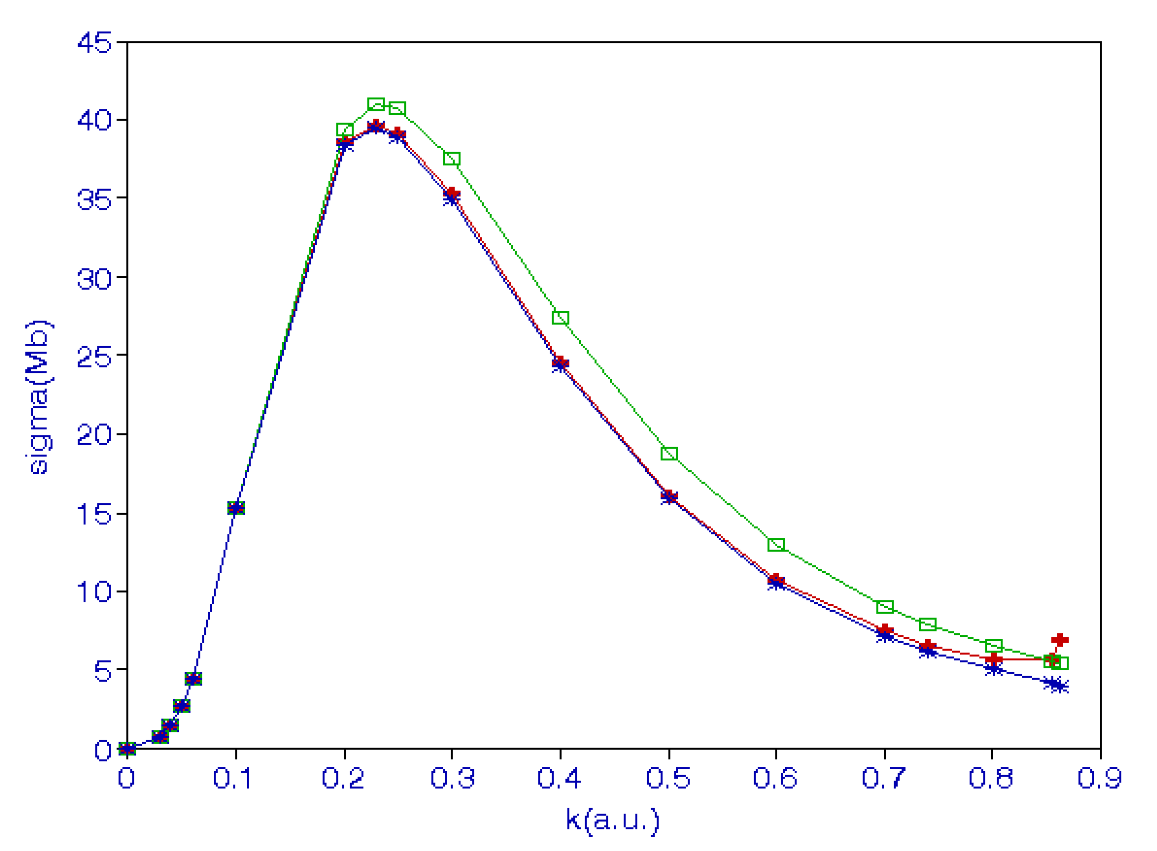
| k | Hybrid Theory [32] | PHQ [31] | Wishart [33] |
|---|---|---|---|
| 0.1 | 15.3024 | 15.400 | 15.937 |
| 0.2 | 38.5443 | 39.411 | 37.870 |
| 0.3 | 35.2318 | 36.639 | 34.239 |
| 0.4 | 24.4774 | 25.296 | 23.858 |
| 0.5 | 16.0858 | 16.473 | 15.720 |
| 0.6 | 10.7410 | 11.601 | 10.431 |
| 0.7 | 7.4862 | 7.587 | 7.101 |
| 0.8 | 5.6512 | 6.456 | 4.978 |
| k | Hybrid Theory [32] | R-Matrix [36] | Experiment [37] |
|---|---|---|---|
| 0.1 | 7.3300 | 7.295 | 7.44 |
| 0.2 | 7.1544 | 7.115 | 7.13 |
| 0.3 | 6.8716 | 6.838 | 6.83 |
| 0.4 | 6.4951 | 6.474 | 6.46 |
| 0.5 | 6.0461 | 6.006 | 6.02 |
| 0.6 | 5.5925 | 5.535 | 5.55 |
| 0.7 | 5.0120 | 4.995 | 5.04 |
| 0.8 | 4.4740 | 4.482 | 4.51 |
| 1.0 | 3.4654 | 3.476 | 3.48 |
| 1.1 | 3.0206 | 3.023 | 3.00 |
| 1.3 | 2.2561 | 2.271 | 2.19 |
| 1.4 | 1.9821 | 1.943 | 1.89 |
| k | [32] | [38] |
|---|---|---|
| 0.2 | 2.5677 | 2.501 |
| 0.3 | 2.5231 | 2.432 |
| 0.4 | 2.4373 | 2.355 |
| 0.5 | 2.3970 | 2.271 |
| 0.6 | 2.2988 | 2.182 |
| 0.7 | 2.0005 | 2.087 |
| 0.8 | 2.0925 | 1.988 |
| 0.9 | 1.9792 | 1.885 |
| 1.0 | 1.8613 | 1.780 |
| 1.1 | 1.7396 | 1.674 |
| 1.2 | 1.6219 | 1.566 |
| 1.3 | 1.5035 | 1.459 |
| 1.4 | 1.3879 | 1.353 |
| 1.5 | 1.2768 | 1.248 |
| 1.6 | 1.1706 | 1.146 |
| N | L | Asymptotic | Variational |
|---|---|---|---|
| 5 | 4 | −4677.0562 | −4676.93484501 |
| 8 | −1391.4385 | −1391.4401873 | |
| 10 | −741.8875 | −741.8935917 | |
| 8 | 5 | −472.5483 | −472.5451674 |
| 10 | −257.9853 | −257.9830286 | |
| 8 | 6 | −187.82161 | −187.821493674 |
| 10 | −105.82980 | −105.829683489 | |
| 9 | 7 | −63.0915572 | −63.0915519990 |
| 10 | −48.6065203 | −48.606514337 |
| Interval | Experiment-Theory | Standard Deviation |
|---|---|---|
| 10G–0H | 0.02 | 0.11 |
| 10H–10I | 0.0003 | 0.0048 |
| System | ln(K) | [58] |
|---|---|---|
| He | 4.367578 | 4.364 |
| Li+ | 5.177763 | 5.177 |
| Be+2 | 5.753615 | 5.754 |
| Ne+8 | 7.586072 | 7.585 |
| L = 4 | L = 5 | L = 6 | L = 7 | L = 8 | L = 9 |
|---|---|---|---|---|---|
| 0.0653658 | 0.0212477 | 0.00790948 | 0.00325464 | 0.00142682 | 0.000646286 |
| N | Energy (a.u.) | fN | |
|---|---|---|---|
| 3 | −7.442225 | 3.2852 | 3.1177 |
| 6 | −7.445404 | 3.0018 | 2.8608 |
| 10 | −7.445413 | 3.0057 | 2.8644 |
| 16 | −7.446614 | 3.0339 | 2.8855 |
| 20 | −7.469530 | 3.0001 | 2.8352 |
| 24 | −7.469904 | 3.0003 | 2.8261 |
| 34 | −7.470761 | 3.0539 | 2.8782 |
| 40 | −7.473393 | 3.0717 | 2.9014 |
| 100-term a | −7.478025 | 2.906 | |
| Experiment b | −7.478069 | 2.9062 | |
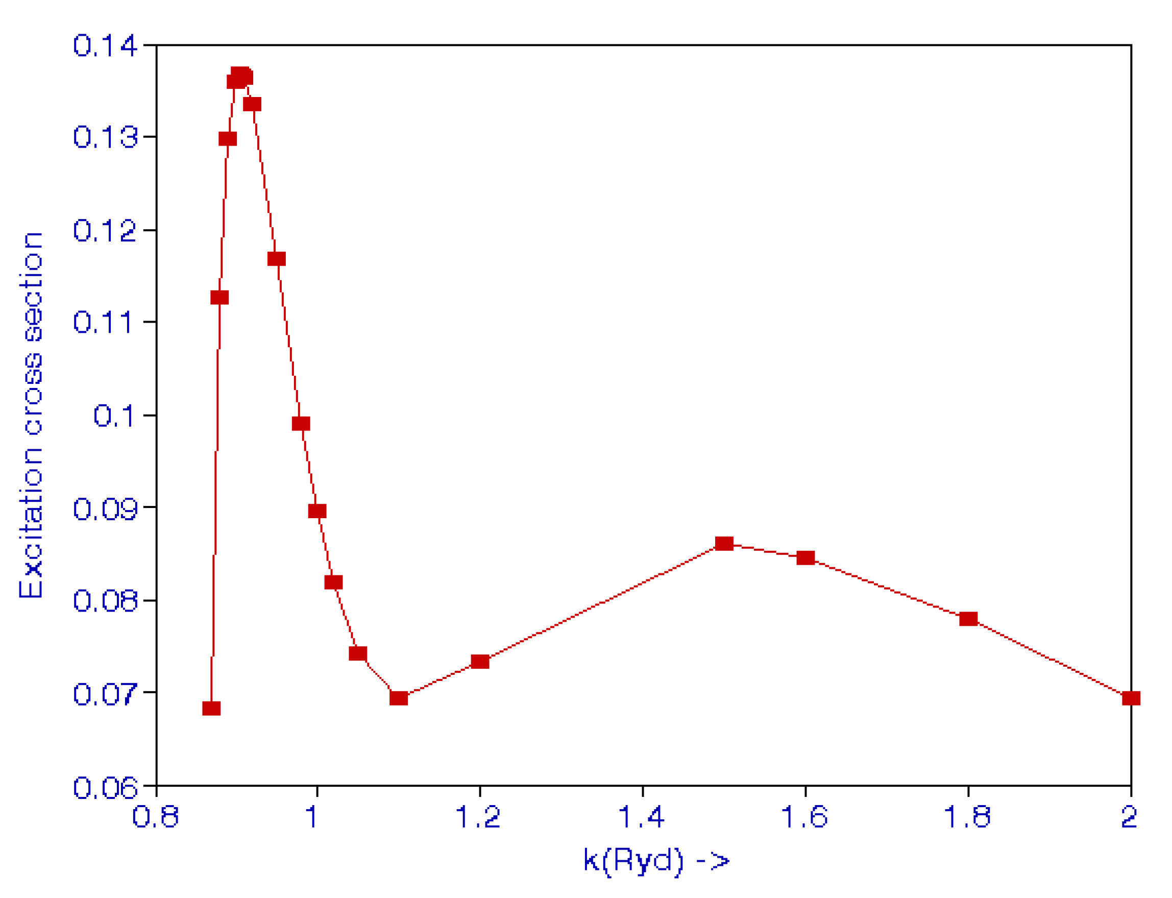
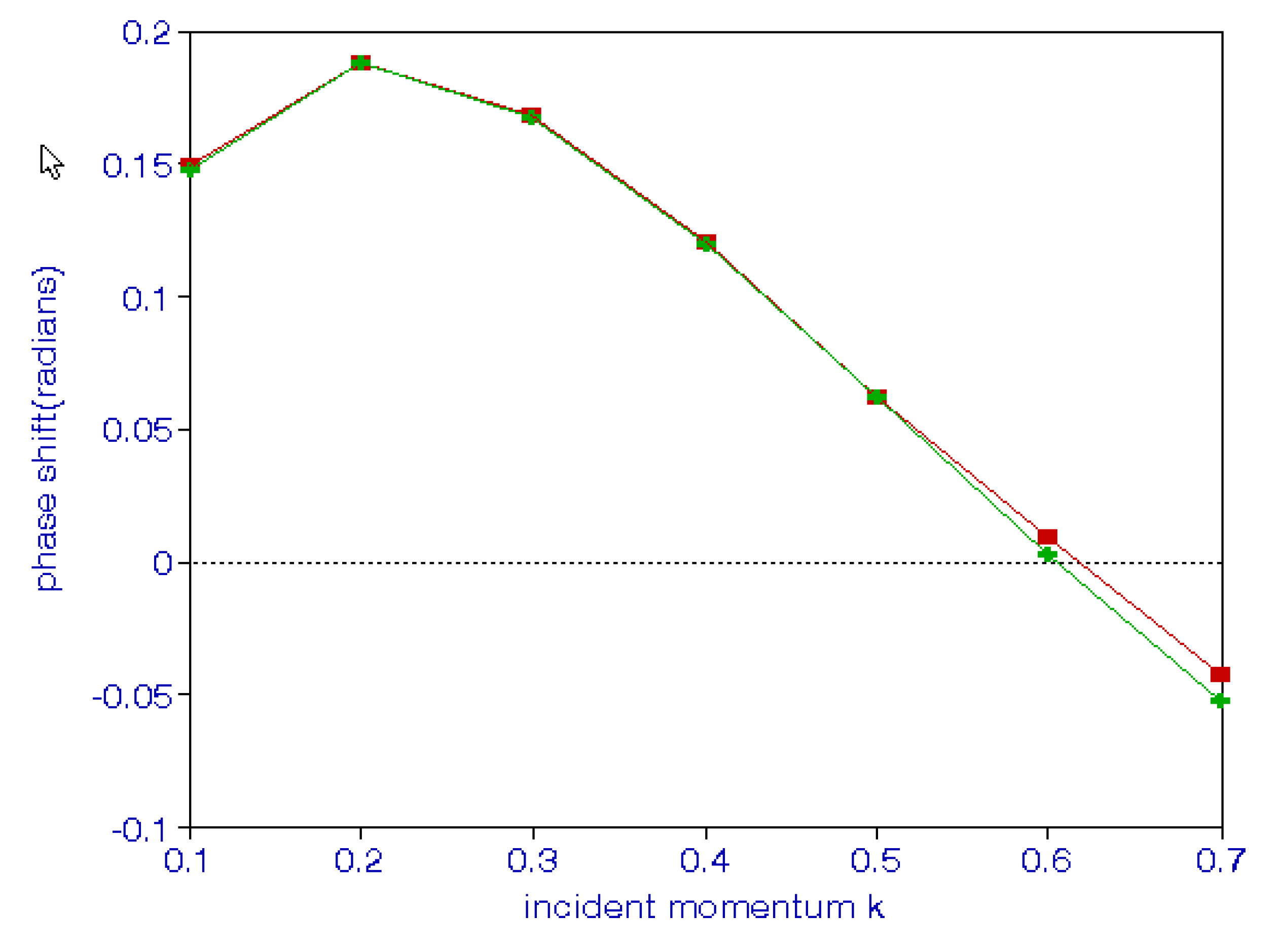
| k | [67] | [66] | [17] | [70] | [69] |
|---|---|---|---|---|---|
| S-wave | P-wave | ||||
| 0.1 | 0.14918 | 0.1483 | 0.151 | 0.008871 | 0.00876 |
| 0.2 | 0.18803 | 0.1877 | 0.188 | 0.032778 | 0.03251 |
| 0.3 | 0.16831 | 0.1677 | 0.168 | 0.06964 | 0.06556 |
| 0.4 | 0.12083 | 0.1201 | 0.120 | 0.10047 | 0.1005 |
| 0.5 | 0.06278 | 0.0624 | 0.062 | 0.13064 | 0.13027 |
| 0.6 | 0.00903 | 0.0039 | 0.007 | 0.15458 | 0.15410 |
| 0.7 | −0.04253 | −0.0512 | −0.54 | 0.17806 | 0.17742 |
| k | L = 0 | L = 1 | L > 1 | Total | ||
|---|---|---|---|---|---|---|
| [67] | [66] | [72] | [70] | |||
| 0.1 | 7.363 | 7.5 | 7.5 | 0.13008 | <0.001 | 7.494 |
| 0.2 | 5.538 | 5.7 | 5.5 | 0.53994 | 0.001 | 6.078 |
| 0.3 | 4.184 | 4.3 | 4.1 | 1.12441 | 0.004 | 5.312 |
| 0.4 | 3.327 | 3.3 | 3.5 | 1.76293 | 0.010 | 5.100 |
| 0.5 | 2.730 | 2.7 | 3.0 | 2.33910 | 0.022 | 5.091 |
| 0.6 | 2.279 | 2.3 | 2.8 | 3.84988 | 0.039 | 4.168 |
| 0.7 | 1.850 | 2.2 | 3.67030 | 0.063 | 5.583 | |
| A | B | C | D | E | |
|---|---|---|---|---|---|
| 0.5041 | 0.0010053 | 0.0066228 | 0.009037 | 0.0041 | 0.0038 |
| 0.5476 | 0.0025753 | 0.018783 | |||
| 0.5625 | 0.0026829 | 0.020249 | 0.024795 | 0.0044 | 0.0041 |
| 0.64 | 0.0025604 | 0.022566 | 0.0248 | 0.0049 | 0.0047 |
| 0.6724 | 0.002412 | 0.022350 | |||
| 0.7225 | 0.0021366 | 0.021456 | 0.021164 | 0.0058 | |
| 0.75 | 0.0020034 | 0.020835 | 0.019707 | ||
| 0.81 | 0.0017211 | 0.019256 | |||
| 0.9025 | 0.0013698 | 0.016760 | |||
| 1.00 | 0.0010916 | 0.014327 |
| Number of Terms | Position | Γ/2 |
|---|---|---|
| 286 | −0.2573744 | 0.0000676 |
| 364 | −0.2573733 | 0.0000674 |
| 455 | −0.2573745 | 0.0000671 |
| 560 | −0.2573740 | 0.0000677 |
| 680 | −0.2573741 | 0.0000677 |
| Threshold n | Position | Width | Position | Width |
|---|---|---|---|---|
| Singlet states | Triplet states | |||
| 2 | 4.7340 | 0.00117 | 5.0742 | 0.000136 |
| 5.0709 | 0.000274 | |||
| 3 | 7.7646 | 0.00204 | 6.0038 | 0.000272 |
| 5.9908 | 0.00150 | |||
| 4 | 6.2526 | 0.00327 | 6.3383 | 0.000272 |
| 6.3267 | 0.00408 | |||
| 6.3317 | 0.00463 | |||
| 5 | 6.4519 | 0.00612 | ||
| 6.4723 | 0.00191 | |||
| Threshold n | Position (Ry) | Width (Ry) |
|---|---|---|
| 2 | −0.12440 a | 0.00054 |
| 3 | −0.063261 | 3.58(−4) |
| −0.0562095 | 5.78(−5) | |
| 4 | −0.037789236 | 3.01(−5) |
| −0.0033087 | 1.8(−6) | |
| 5 | −0.03090972 a | 6.4(−5) |
| −0.02493166 | 5.09(−5) | |
| −0.0220972 | 5.24(−5) | |
| −0.021660 | 2.64(−5) | |
| 6 | −0.017596 | 1.06(−4) |
| −0.015894 | 1.6(−4) | |
| −0.015811 | 1.14(−4) | |
| −0.013761 | 4.0(−5) |
| Threshold | Position (Ry) | Width (Ry) |
|---|---|---|
| 3 | −0.05450 | 9.20(−4) |
| 5 | −0.01971 | 6.60(−5) |
| 7 | −0.01008 | 4.00(−5) |
| Threshold | Position (Ry) | Width (Ry) |
|---|---|---|
| 2 | −0.12434 | 9.00(−4) |
| 4 | −0.030975 | 6.00(−5) |
| 6 | −0.01375 | 5.20(−5) |
| E (eV) | e–He | e+–He |
|---|---|---|
| 50 | 1.27 | 1.97 |
| 100 | 1.16 | 1.26 |
| 150 | 0.967 | 0.987 |
| 200 | 0.796 | 0.812 |
| 300 | 0.614 | 0.612 |
| 500 | 0.437 | 0.434 |
| 600 | 0.371 | 0.381 |
| 0.6 | 0.8 | 0.6 | 0.8 | ||
|---|---|---|---|---|---|
| Electrons | Positrons | ||||
| 0.001 | 911,300 | 2.71(−23) | 3.64(−23) | 1.30(−24) | 2.27(−24) |
| 0.003 | 303,766.7 | 3.01(−24) | 4.05(−24) | 1.44(−25) | 2.52(−25) |
| 0.005 | 182,260 | 7.51(−25) | 1.46(−24) | 5.19(−26) | 9.06(−26) |
| 0.01 | 91,130 | 2.71(−25) | 3.64(−25) | 1.30(−26) | 2.27(−26) |
| 0.02 | 45,565 | 6.77(−26) | 9.09(−26) | 3.33(−27) | 1.02(−26) |
| 0.03 | 30,376.7 | 3.01(−26) | 4.04(−26) | 1.52(−27) | 2.65(−27) |
| 0.04 | 22,782.5 | 1.70(−26) | 2.27(−26) | 8.89(−28) | 1.53(−27) |
| 0.05 | 18,226 | 1.34(−26) | 1.45(−26) | 5.90(−28) | 1.01(−27) |
| 0.06 | 15,188.3 | 7.56(−27) | 1.01(−26) | 4.25(−28) | 7.26(−28) |
| 0.08 | 11,391.3 | 4.27(−27) | 6.44(−27) | 2.56(−28) | 4.32(−28) |
| 0.10 | 9113 | 2.74(−27) | 3.63(−27) | 1.48(−28) | 3.50(−28) |
| 0.5 | 0.6 | 0.7 | 0.8 | 0.9 | 1.0 | 1.4 | 1.6 | 1.8 | 2.0 | |
|---|---|---|---|---|---|---|---|---|---|---|
| Present | 2.22 | 2.71 | 3.18 | 3.64 | 4.09 | 4.53 | 6.19 | 6.95 | 7.68 | 8.36 |
| [99] | 2.28 | 2.78 | 3.25 | 3.70 | 4.15 | 4.59 | 6.30 | 7.10 | 7.90 | 8.70 |
| [100] | 20.2 | 22.4 | 24.4 | 26.1 | 27.8 | 29.4 | 35.0 | 37.6 | 40.8 | 42.3 |
| Present | 0.56 | 0.68 | 0.79 | 0.91 | 1.02 | 1.13 | 1.57 | 1.10 | 1.97 | 2.17 |
| [99] | 0.57 | 0.69 | 0.81 | 0.92 | 1.03 | 1.15 | 1.57 | 1.10 | 1.97 | 2.17 |
| [100] | 2.77 | 3.12 | 3.45 | 3.76 | 4.06 | 4.36 | 5.49 | 6.05 | 6.60 | 7.14 |
| Cf. of Electron + H | Cf. of Positron + H | Cf. of Positron + Ps | ||||
|---|---|---|---|---|---|---|
| 0.10 | 9113 | 4.13(−17) | 3.63(−27) | 2.90(−28) | 4.17(−17) | 7.41(−27) |
| 0.08 | 11,391.25 | 3.34(−17) | 5.66(−27) | 4.32(−28) | 5.82(−17) | 1.13(−26) |
| 0.07 | 13,018.57 | 2.32(−17) | 7.34(−27) | 5.49(−28) | 7.12(−17) | 1.46(−26) |
| 0.065 | 14,020 | 1.57(−17) | 8.58(−27) | 6.28(−28) | 7.95(−17) | 1.68(−26) |
| 0.06 | 15,188.33 | 7.05(−18) | 1.01(−26) | 7.26(−28) | 8.96(−17) | 1.96(−26) |
| 0.05 | 18,226 | 0.00 | 1.45(−26) | 1.01(−27) | 1.18(−16) | 2.78(−26) |
| 0.04 | 22,782.5 | 0.00 | 2.27(−26) | 1.53(−27) | 1.65(−16) | 4.29(−26) |
| 0.03 | 30,376.67 | 0.00 | 4.04(−26) | 2.65(−27) | 2.53(−16) | 7.54(−26) |
| 0.02 | 45,565 | 0.00 | 9.09(−26) | 5.80(−27) | 4.64(−16) | 1.68(−25) |
| 0.015 | 60,753.33 | 0.00 | 1.62(−25) | 1.02(−26) | 7.13(−16) | 2.97(−25) |
| 0.01 | 91,130 | 0.00 | 3.64(−25) | 2.27(−26) | 1.30(−15) | 6.66(−25) |
| 0.005 | 182,260 | 0.00 | 1.01(−25) | 6.30(−26) | 3.63(−15) | 2.66(−24) |
| 0.003 | 303,766.7 | 0.00 | 4.05(−24) | 2.52(−25) | 7.69(−15) | 7.39(−24) |
| 0.001 | 911,300 | 0.00 | 3.64(−23) | 2.27(−24) | 3.55(−14) | 6.66(−23) |
Publisher’s Note: MDPI stays neutral with regard to jurisdictional claims in published maps and institutional affiliations. |
© 2020 by the author. Licensee MDPI, Basel, Switzerland. This article is an open access article distributed under the terms and conditions of the Creative Commons Attribution (CC BY) license (http://creativecommons.org/licenses/by/4.0/).
Share and Cite
Bhatia, A.K. Scattering and Its Applications to Various Atomic Processes: Elastic Scattering, Resonances, Photoabsorption, Rydberg States, and Opacity of the Atmosphere of the Sun and Stellar Objects. Atoms 2020, 8, 78. https://0-doi-org.brum.beds.ac.uk/10.3390/atoms8040078
Bhatia AK. Scattering and Its Applications to Various Atomic Processes: Elastic Scattering, Resonances, Photoabsorption, Rydberg States, and Opacity of the Atmosphere of the Sun and Stellar Objects. Atoms. 2020; 8(4):78. https://0-doi-org.brum.beds.ac.uk/10.3390/atoms8040078
Chicago/Turabian StyleBhatia, Anand K. 2020. "Scattering and Its Applications to Various Atomic Processes: Elastic Scattering, Resonances, Photoabsorption, Rydberg States, and Opacity of the Atmosphere of the Sun and Stellar Objects" Atoms 8, no. 4: 78. https://0-doi-org.brum.beds.ac.uk/10.3390/atoms8040078