Article

Plasma Spectroscopy on an Aluminum-Pellet Ablation Cloud in an LHD Plasma with an Echelle Spectrometer

1
Department of Mechanical Engineering and Science, Graduate School of Engineering, Kyoto University, Kyoto 615-8540, Japan
2
National Institute for Fusion Science, 322-6 Oroshi-cho, Toki, Gifu 5909-5292, Japan
*
Author to whom correspondence should be addressed.
Submission received: 16 September 2020 / Revised: 20 October 2020 / Accepted: 11 November 2020 / Published: 13 November 2020
(This article belongs to the Special Issue Atomic and Molecular Spectra in Magnetically Confined Torus Plasmas)

Abstract

:
We developed an echelle spectrometer for the simultaneous observation of the whole visible range with a high instrumental resolution, for example, 0.055 nm (full width at the half maximum) at 400 nm and 0.10 nm at 750 nm. With the spectrometer, the emission from an ablation cloud of an aluminum pellet injected into a high-temperature plasma generated in the Large Helical Device (LHD) was measured. We separated the emission lines into Al I, II, III and IV groups, and estimated the electron temperature and density of the ablation cloud from the line intensity distribution and Stark broadening respectively, of each of the Al I, II and III groups. We also determined the Stark broadening coefficients of many Al II and III lines from the respective Stark widths with the estimated electron temperature and density.

1. Introduction

A pellet injected into a high-temperature plasma is immediately ablated due to heat flux from the plasma and forms a high-density plasma called an ablation cloud. From the ablation cloud, many atomic and ionic line emissions are observed. Spectroscopic studies of the emissions may offer information about not only atomic data and possibility of new light sources, but also the ablation mechanism and atomic processes therein, and transport in the main plasma. In the Large Helical Device (LHD), for example, pellets of carbon, aluminum, titanium, tin, tungsten bismuth and so on have been injected to examine the dependence of transport coefficients, the emissivity and peak wavelength on the atomic number [1,2,3], owing to its capability to generate stable high-temperature plasmas.
With an assumption that intensity of line emissions from the ablation cloud is proportional to the ablation rate, trajectory of the pellet or shape of the clouds is deduced from the temporal variation of the emission intensity [4,5,6,7,8]. Detailed information about atomic processes taking place in the ablation cloud is necessary for more quantitative understanding of the ablation mechanism. Wideband spectra containing many emission lines have been measured for hydrogen, carbon and aluminum pellets [9,10,11]. From such measurements with intensity ratio analysis of the emission lines, population distribution of excited levels of atoms or ions in the ablation cloud has been investigated and plasma parameters such as electron temperature, neutral atom density and ion density have been estimated. In addition to such wideband measurements, high-resolution spectra of the emission lines have been measured for carbon pellets [10], and the electron density of the cloud has been estimated from the Stark broadening.
It may be desired to perform both the wideband and high-resolution measurements simultaneously for a single pellet injection because ablation clouds are not necessarily in the same condition, even if similar pellets are injected into similar plasmas. However, it is not easy to perform both types of measurements simultaneously. Moreover, in the case of metal elements, the emission lines are so crowded that it is hard to resolve them with an ordinary low-dispersion spectrometer. In fact, in the spectroscopic study on an aluminum pellet [11], the number of discretely measured lines and the accuracy of their intensities were limited by the resolution of the spectrometer.
For the purpose of overcoming this problem, we have developed an echelle spectrometer by ourselves and applied it to study an aluminum pellet ablation cloud generated in the LHD [12]. In this special issue, we report details of the spectrometer and systematic analysis of the Stark broadening coefficient of aluminum ions with the results shown in Reference [12].

2. Experimental Setup

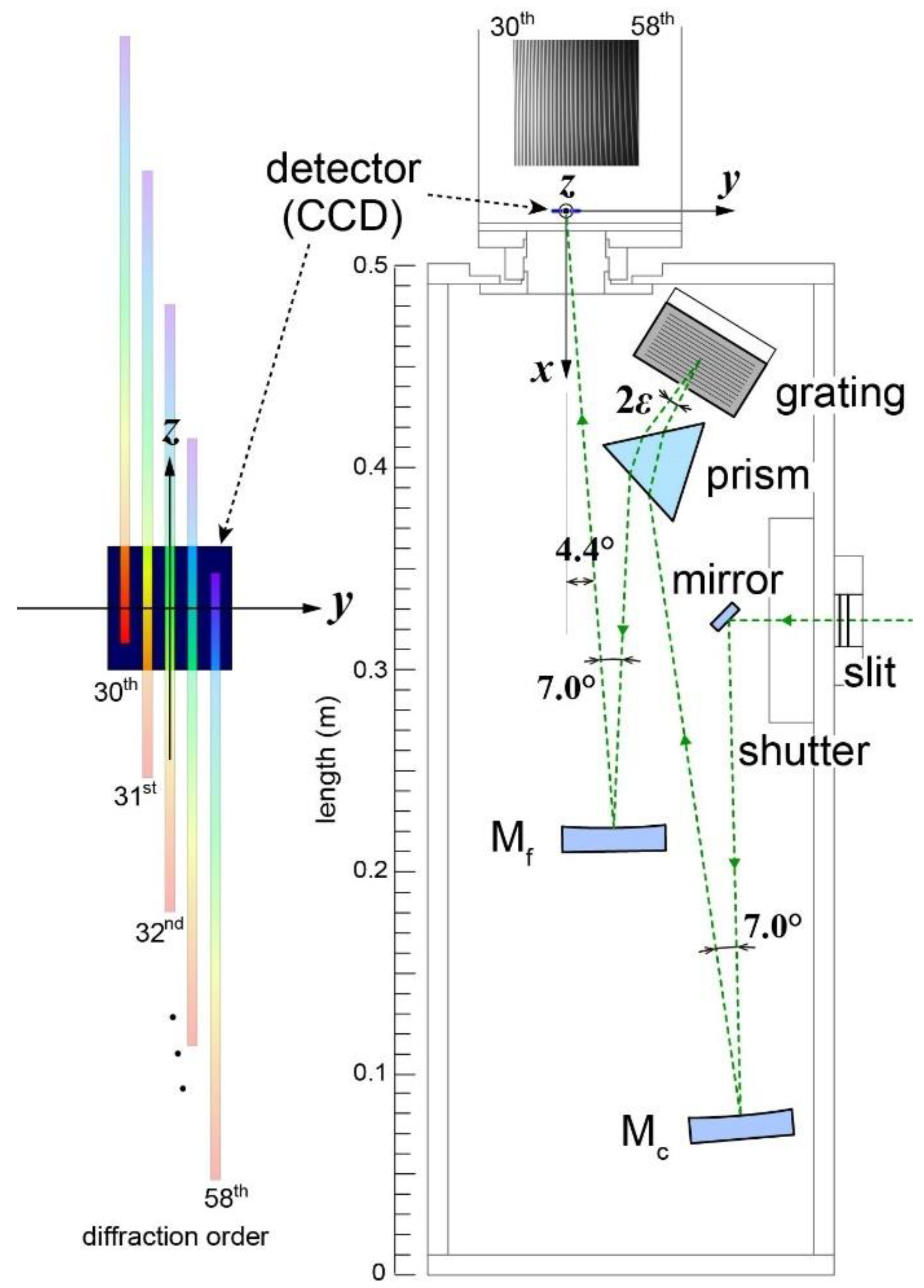
Figure 1 shows a schematic illustration of the echelle spectrometer developed for the present study and x-, y- and z-axes defined for the explanation. Emission light passed through the entrance slit is reflected by a mirror and collimated by a concave mirror, Mc (focal length: 304.8 mm). The parallel light beam is diffracted in the z-direction by an echelle grating (Newport, 46.1 grooves mm−1, 32° blaze) according to their wavelength, but light beams of many diffraction orders overlap each other. These overlapping light beams are spatially separated by a 60° quartz prism in the direction perpendicular to the z-direction. Finally, separated 30th–58th diffraction light beams are focused on a charge-coupled device (CCD) camera (Andor, DV435-BV, 1024 × 1024 pixels) along the y-direction by another concave mirror, Mf (focal length: 304.8 mm). A typical two-dimensional image taken by the CCD camera for white light emission from a deuterium lamp is shown in the top of Figure 1. The CCD is cooled to be −25 °C to reduce thermal noise.
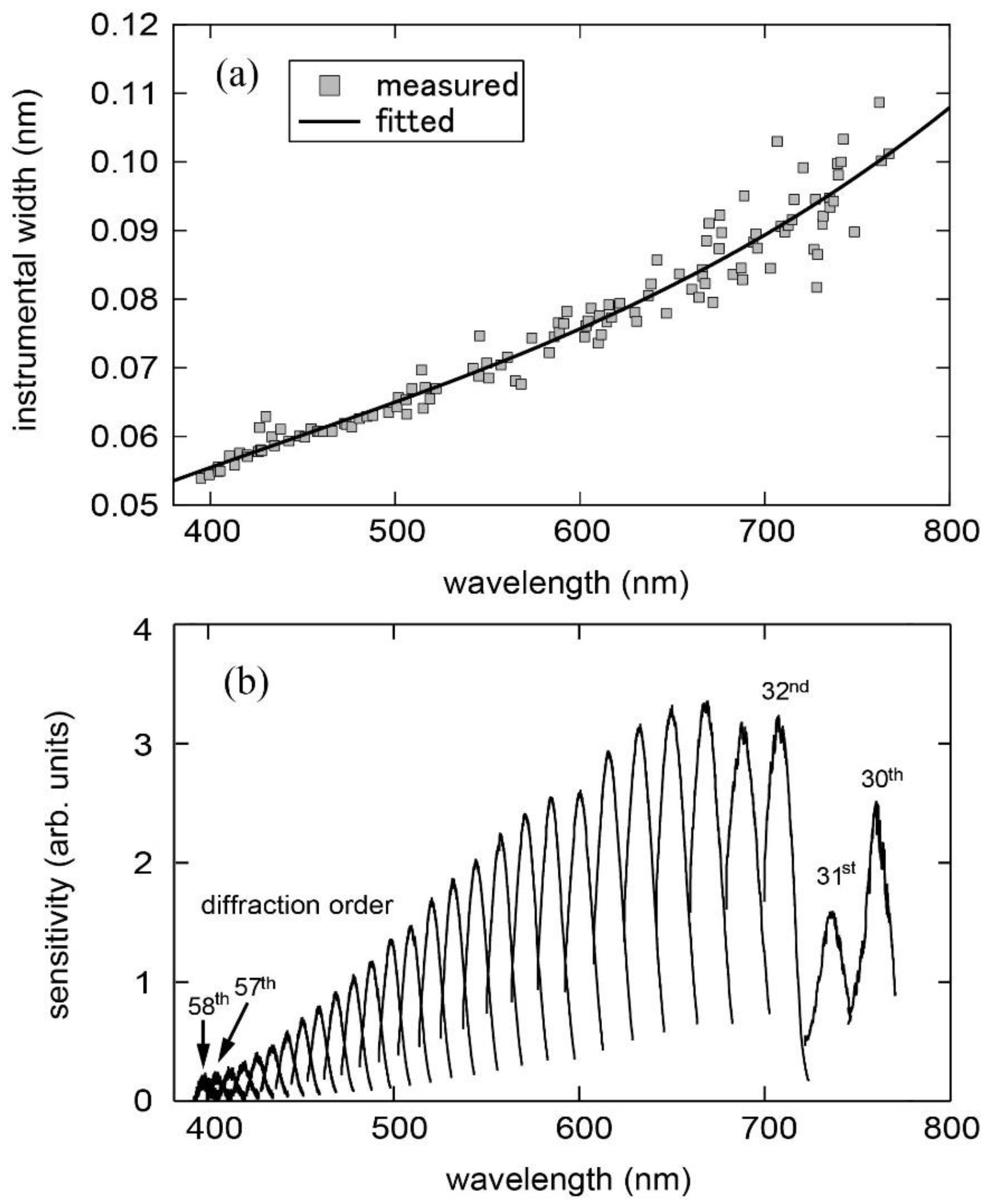
For the purpose of wavelength calibration and resolution estimation, we measure emission lines of a Th-Ar hollow cathode lamp (Heraeus, P858A) [12] because it has many emission lines in the visible region and the line widths are small enough. The instrumental function of the spectrometer is found to be approximated by a Gaussian profile. We evaluate the instrumental width (full width at the half maximum) by fitting bright Th and Ar lines with a Gaussian function. Figure 2a shows the evaluated width at the entrance slit width of 25 μm as a function of the wavelength. The curve in the figure is the result of the fit with a third-order polynomial function. We use this fitted curve as the instrumental width at an arbitrary wavelength in the spectral shape analysis explained later. We also calibrate the relative sensitivity of the spectrometer for the whole wavelength region using a tungsten standard lamp with an integrating sphere (Labsphere, USS-600C, North Sutton, NH, USA) [12]. The result of the sensitivity calibration is shown in Figure 2b.
The LHD has a torus-shape vacuum vessel with a major radius of about 3.9 m and a minor radius of about 1 m, in which a plasma of about 30 m3 is confined. The confinement magnetic field is produced by a pair of superconducting helical coils and three pairs of superconducting poloidal coils. The plasma is heated by electron cyclotron heating, ion cyclotron resonance heating and neutral beam injection. For the pellet ablation measurement, we use a pure Al pellet having a cylindrical shape whose diameter and length are 0.8 mm [12]. The pellet is accelerated in a 6 m long acceleration tube with a pneumatic pipe-gun system, which uses a helium gas of 18 atm pressure, and then injected horizontally into the plasma from an outer port of the LHD (1-O port). Figure 3 shows a schematic illustration for a part of the equatorial plane of the LHD, in which the pellet trajectory is indicated by a dashed arrow. The travelling speed of the pellet is known to be about 200 ms−1 from the time-of-flight measurement for a carbon pellet [10]. The LHD shot number is 104,159, in which the major radius position of the magnetic axis and the field strength are set to be 3.90 m and 2.54 T, respectively [12].
We place a lens having a focal length of 10 mm and an optical fiber having a core diameter of 1 mm at an observation port close to the pellet acceleration tube. The line of sight is parallel to the injection direction of the pellet, as shown in Figure 3. Emission from the ablation cloud is focused on one end of the optical fiber by the lens, relayed by several optical fibers having a core diameter of 0.3 mm, and introduced to the entrance slit of the spectrometer. Since the exposure time of the CCD camera is set to be 95 ms, which is much longer than the period of luminous radiation from the ablation cloud of several ms, time-integrated emission during the pellet ablation is measured.

3. Results and Discussion

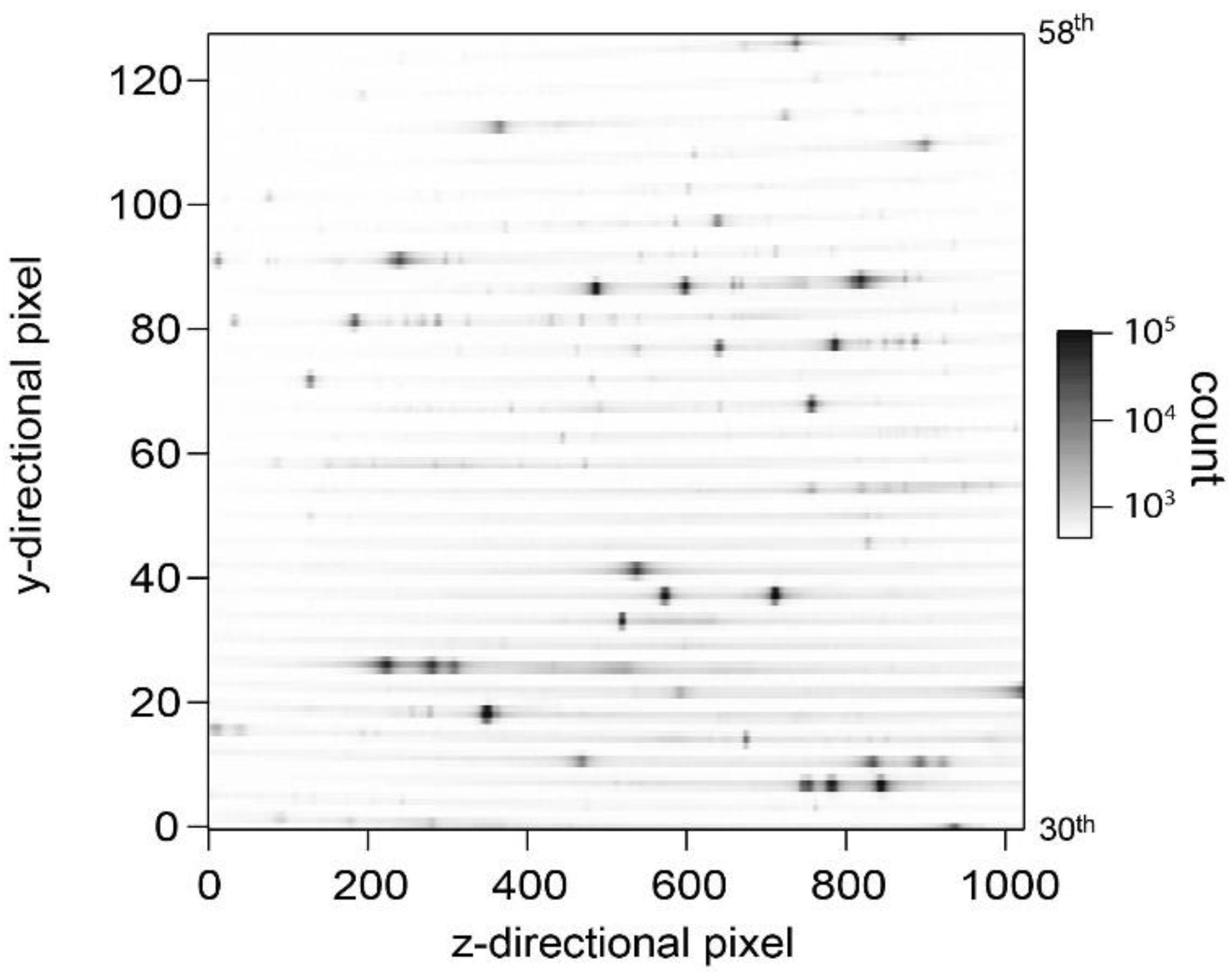
Figure 4 shows a two-dimensional image taken by the CCD camera for the emission from the aluminum pellet ablation cloud. It is noted that since 8-pixel binning in the y-direction is done to shorten the readout time of the data, the image consists of 128 × 1024 pixels. We also take a background image when there is no plasma emission.
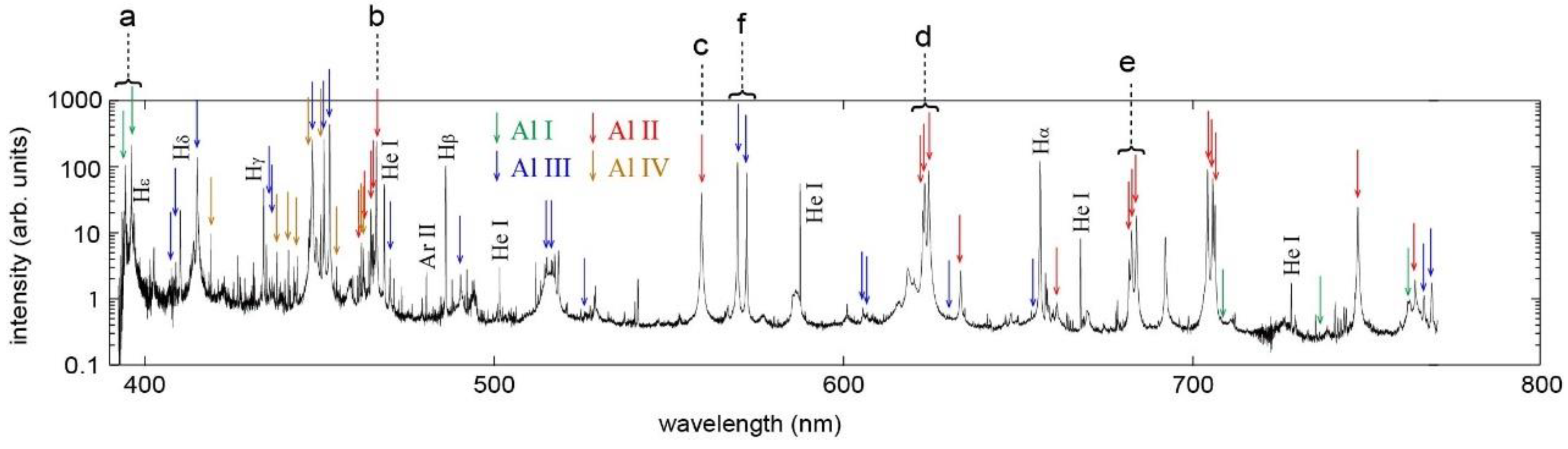
By subtracting the background from the data shown in Figure 4, separating the spectra with respect to the diffraction orders, calibrating wavelength and relative sensitivity, and arranging the spectra according to the wavelength, we obtain the spectrum shown in Figure 5 [12]. It is noted that the intensity in the figure is in a logarithmic scale.
More than 100 emission lines are resolved, in which more than 50 lines are identified as Al I, Al II, Al III and Al IV lines from available databases [13,14]. The identified lines are indicated in Figure 5 by arrows and listed in Table 1, Table 2, Table 3 and Table 4. The lines denoted by ‘a–f’ are used to estimate electron density of the ablation cloud from their Stark width, as explained below. Since the LHD plasma contains hydrogen, helium, argon, etc., emission lines of these elements are also seen in Figure 5.
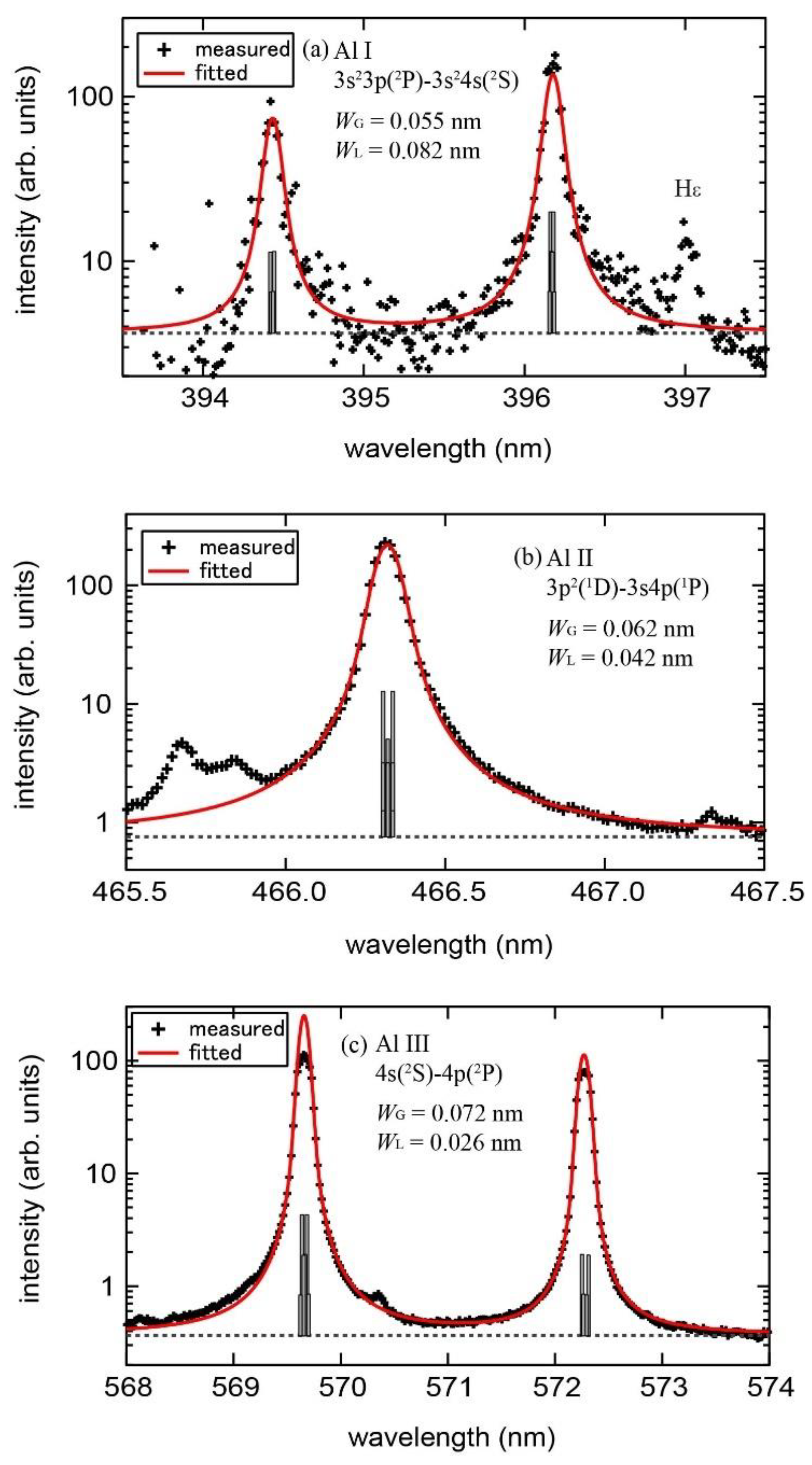
Many of the observed lines are found to show broadenings, which cannot be reproduced by a Gaussian profile [12]. The broadenings may be mainly due to Stark broadening having a Lorentzian profile because electron density in the ablation cloud is expected to be high. Furthermore, influence of the Zeeman splitting on the line profile may not be negligible. We fit the observed line profiles as follows: we calculate the splitting and relative emission intensities of the Zeeman components with the method based on the perturbation theory for B = 1.5   T , which is approximate magnetic field strength at the location where the radiation intensity of the ablation cloud will take its maximum, and then fit the line profile by a sum of several shifted Voigt functions according to the Zeeman splitting, which have a common Lorentz width, W L , and a fixed Gaussian width, W G , determined as the instrumental width shown by the curve in Figure 2a. The adjustable parameters for the fit are W L and the area of the spectrum. Examples of the observed spectra and the result of the fit are shown in Figure 6. In the fit, we use the least square method with weighting the accuracy of the data point in the spectrum estimated from the shot noise of the signal intensity with the dark current noise and the uncertainty of the intensity calibration. It is noted here that the large scatter of the data points in Figure 6a is due to the low sensitivity of the spectrometer at the wavelength around 395 nm, because the wavelength is not only in the low sensitivity region but also in between the 57th and 58th diffraction orders of the spectrometer (see Figure 2b). The sensitivity is more than one order of magnitude smaller than those for Figure 6b,c. Additionally, since the hydrogen, Hε, emission line of 397 nm is detected, we mask the Hε spectrum in the line profile fit. In the spectra shown in Figure 6b, there are unidentified emission lines in 465.5–466.0 nm, where the spectra are masked for the line profile fit. The possible candidates of the unidentified lines are Fe I 465.64570, 465.75845 and 465.82944 nm, and Fe II 465.6981 nm. On the other hand, since saturation around the emission peaks due to the radiation reabsorption is detected for the Al III 4s(2S)–4p(2P) line, as seen in Figure 6c, we mask the spectra around the emission peaks in the line profile fit.
Emission line intensity is given as the area of the line spectrum. The line intensity, I ( p , q ) , from a level p to a level q is proportional to the upper level population, n ( p ) , as
I ( p , q ) = h ν ( p , q ) A ( p , q ) n ( p ) ,
where h is Planck’s constant. ν ( p , q ) and A ( p , q ) 
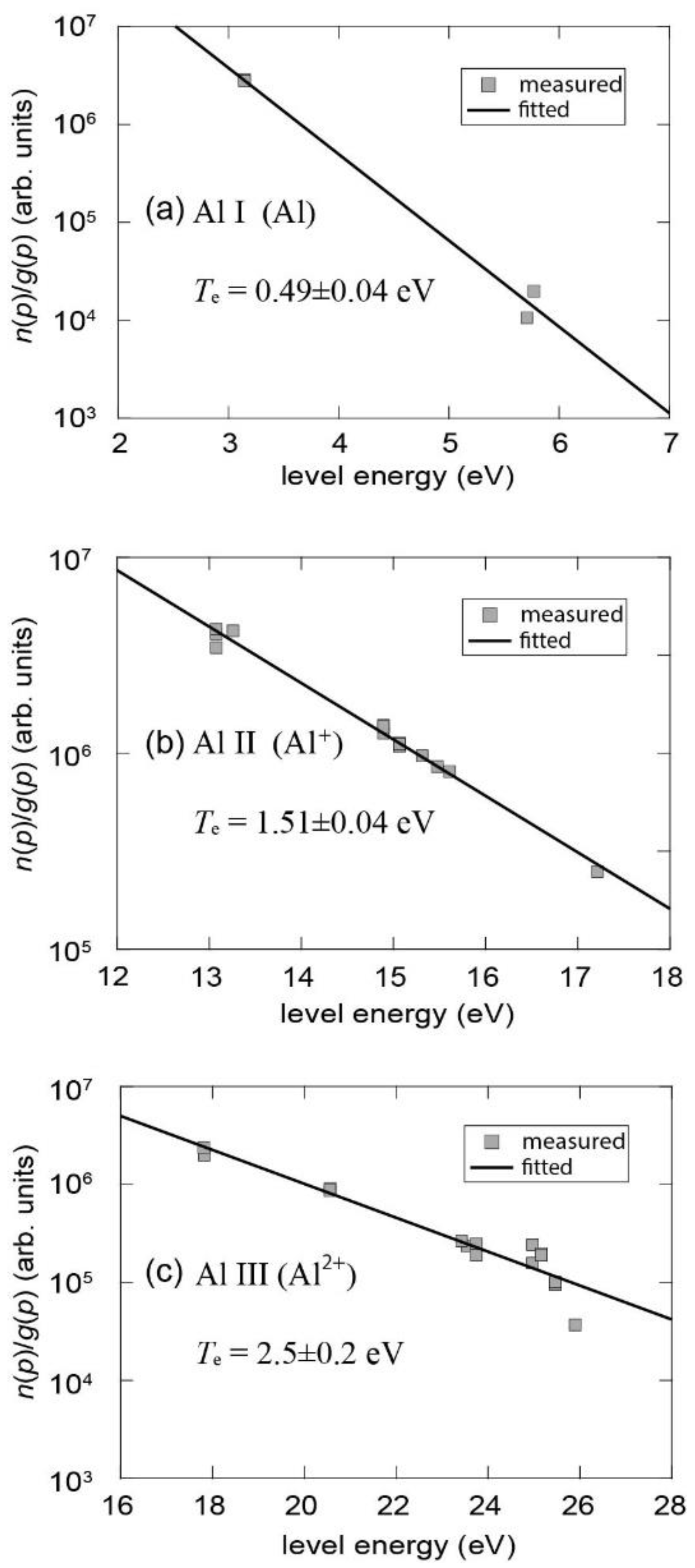
are the frequency of light and the spontaneous transition probability, respectively. Populations of excited levels of atoms and ions in the ablation cloud can be estimated from the observed line intensities with Equation (1) for well-resolved emission lines, enough to evaluate the area of the spectra having available transition probabilities [13,14]. The results for neutral aluminum atoms (Al), singly ionized aluminum ions (Al+) and doubly ionized aluminum ions (Al2+) are shown in Figure 7 by the Boltzmann plot against the upper level energy [12]. It is clear that the population distribution can be fitted with a straight line for each charge state.
It is known that in the case where atoms or ions of an excited level p in a plasma are in the local thermodynamic equilibrium (LTE), population of p follows the Saha-Boltzmann distribution:
n z ( p ) g z ( p ) = 1 2 ( h 2 2 π m k T e ) 3 / 2 exp ( χ z ( p ) k T e ) n e n z + 1 ( 1 ) g z + 1 ( 1 ) ,
where m is the electron mass, k is the Boltzmann constant and n z ( p ) , g z ( p ) and χ z ( p ) are the population, statistical weight and ionization potential of a level p respectively, of a charge state AlZ+ [15]. p = 1 stands for the ground state, and n e and T e are the electron density and temperature, respectively. In this case, the upper level populations in the Boltzmann plot are on a straight line and the slope of the line is determined by the electron temperature. From the straight lines fitted to the population distributions shown in Figure 7, we estimate T e of the ablation cloud for Al, Al+ and Al2+ plasmas. The estimated T e are shown in Figure 7. Validity of the LTE assumption for these plasmas are discussed later.
Regarding the Lorentz width, the natural broadening determined by the spontaneous transition is negligibly small in comparison with the observed width. Therefore, we treated the observed Lorentz width as the Stark width, W s = W L . The Stark width is proportional to the electron density as
W s = C s ( T e ) n e ,
where C s is the Stark broadening coefficient.
W s of the Al I 2s23p(2P)–3s24s(2S) line denoted by ‘a’ in Figure 5 and Table 1 has been calculated for several T e at n e = 1022 m−3, as shown in Figure 8a [16]. The curve in the figure is the fitted result by an exponential function. From the curve, we determine C s of the line at T e = 0.49 eV, which is the electron temperature of the Al plasma. Then, n e of the Al plasma is estimated from the observed W s with the determined C s . The result is shown in Table 5.
A similar analysis can be done for the Al II lines denoted by ‘b’, ‘c’, ‘d’ and ‘e’ in Figure 5 and Table 2. W s determined in previous calculations and experiments at several T e are shown in Figure 8 [16,17,18]. The curves in the figure are the results of the fit with exponential functions. From the curves, we determine C s of the lines at T e = 1.51 eV, which is the electron temperature of the Al+ plasma. Since the experimental data only at T e = 0.9 eV is available for the Al II line denoted by ‘c’, we adopt the value of C s at T e = 0.9 eV as that at T e = 1.51 eV, assuming T e dependence of C s is small in this electron temperature region. The estimated n e from these lines are listed in Table 6 [12]. It is found that the scatter of the values are within 15% of the average. We adopt the average value as the electron density of the Al+ plasma.
Regarding Al III lines, WS of only the line denoted by ‘f’ in Figure 5 and Table 3 was measured at T e = 4.3 eV and n e = 1024 ~ 1025 m−3 [18], as far as the authors know. With the assumption that the difference of C s between T e = 4.3 eV and the Al2+ plasma electron temperature ( T e = 2.5 eV) is negligibly small, we determine C s , and then estimate n e of the Al2+ plasma from the observed W s . The result is shown in Table 7.
In Table 8, we summarize T e and n e of the ablation cloud for Al, Al+ and Al2+ plasmas [12]. It is found that T e increases while n e decreases as an increase in the charge state. This tendency suggests that aluminum in different charge states emits radiation in different regions of the ablation cloud and/or at different times during the ablation. It has been reported, however, that intensity ratios of emission lines of various carbon ions change little during the carbon pellet ablation [10]. Supposing that the ablation mechanism due to heat flux from the LHD main plasma is the same for carbon and aluminum pellets, we attribute the observed tendency to an inhomogeneous structure of the ablation cloud. The plasma region for neutral atoms is close to the ablating pellet, where n e is high and T e is low and the region for a higher charge state is farther from the pellet where the cloud is expanding in the LHD main plasma with increasing T e and decreasing n e .
Here, we discuss the validity of the LTE assumption. It is known that the necessary condition for excited levels of atoms and ions in a plasma to be the LTE is that electron collision processes are dominant and radiative processes can be negligible. The lowest value of the electron density, which realizes such a situation for all levels of an ionization state, is given as McWhirter’s criterion [19,20]:
n e n c = 1.6 × 10 12 T e 1 2 ( Δ E ) 3 ,
where Δ E is the largest energy gap between two adjacent levels allowed by radiative transition (generally, the energy gap between the ground and first excited states). In Equation (4), the unit of Δ E is eV and those of T e and n e are K and cm−3, respectively.
According to Equation (4), n c for the Al, Al+ and Al2+ plasmas are estimated to be in the orders of 1021, 1022 and 1022 m−3, respectively. Moreover, it is confirmed that a collisional-radiative model calculation [21] shows that almost all the excited levels of Al+ would be in LTE when n e is higher than 1022 m−3 at T e = 1 eV. Since the estimated n e of the Al, Al+ and Al2+ plasmas from the observed Stark widths are higher than these values, it is consistent for the observed population distributions to obey the Saha-Boltzmann distribution.
From the observed Stark widths with T e and ne estimated above, we determine Stark broadening coefficients of Al II and III lines, the values of which have not been reported. The determined values are listed in Table 9 and Table 10 together with the data used for the n e estimation. It is demonstrated that the ablation plasma spectroscopy with a simultaneous wideband and high-resolution measurement can be a powerful tool to acquire atomic data, like Stark broadening coefficients.

4. Conclusions

With developing an echelle spectrometer for the simultaneous measurement of the entire visible region with a high resolution, we observed the emission spectrum of an ablation cloud of an aluminum pellet injected into an LHD plasma. More than 50 of Al I, II, III and IV emission lines were identified in the spectrum. Population distributions of excited levels of atoms and ions in the Al, Al+ and Al2+ plasmas converted from the observed line intensities were analyzed. The LTE states were thought to be generated in the Al, Al+ and Al2+ plasmas and the electron temperatures of the plasmas were estimated. The electron densities of the plasmas were also estimated from the observed Stark widths by comparison with the previously reported Stark widths. It was found that the electron temperature and density increased and decreased respectively, as the charge state of aluminum increased. The phenomenon implies a laminar structure of the ablation cloud: higher density, lower temperature and lower ionized plasma inside, and lower density, higher temperature and higher ionized plasma outside. On the other hand, Stark broadening coefficients of many Al II and III lines were newly determined from the observed Stark widths with the estimated electron density.

Author Contributions

Conceptualization, M.H.; methodology, H.T., K.F., T.S. and M.H.; investigation, H.T., K.F., T.S., S.M., M.G. and M.H.; writing—original draft preparation, H.T. and M.H.; writing—review and editing, M.H.; funding acquisition, S.T. and M.H. All authors have read and agreed to the published version of the manuscript.

Funding

This work has been financially supported by the NIFS Collaborative Research Program NIFS12KLPH017 and by the Grant-in-Aid for Scientific Research, No. 20K20962, from the Japan Society for the Promotion of Science.

Acknowledgments

The authors are grateful to technical staff of the workshop of the department of mechanical engineering and science in Kyoto University for their support in manufacturing of the spectrometer. The support of the LHD experiment group is also greatly acknowledged.

Conflicts of Interest

The authors declare no conflict of interest.

References

  1. Tamura, N.; Sudo, S.; Khlopenkov, K.V.; Kato, S.; Sergeev, V.Y.; Muto, S.; Sato, K.; Funaba, H.; Tanaka, K.; Tokuzawa, T.; et al. Impurity transport studies by means of tracer-encapsulated solid pellet injection in neutral beam heated plasmas on LHD. Plasma Phys. Control. Fusion 2002, 45, 27–41. [Google Scholar] [CrossRef]
  2. Nozato, H.; Morita, S.; Goto, M.; Takase, Y.; Ejiri, A.; Amano, T.; Tanaka, K.; Inagaki, S.; LHD Experimental group. A study of charge dependence of particle transport using impurity pellet injection and high-spatial resolution bremsstrahlung measurement on the Large Helical Device. Phys. Plasmas 2004, 11, 1920–1930. [Google Scholar] [CrossRef]
  3. Ohashi, H.; Higashiguchi, T.; Suzuki, Y.; Arai, G.; Otani, Y.; Yatagai, T.; Li, B.; Dunne, P.; O’Sullivan, G.; Jiang, W.; et al. Quasi-Moseley’s law for strong narrow bandwidth soft x-ray sources containing higher charge-state ions. Appl. Phys. Lett. 2014, 104, 234107. [Google Scholar] [CrossRef]
  4. Yoshiaki, S.; Shigeru, M.; Motoshi, G.; Hiroshi, I.; Noriyuki, I.; Shin, K.; Keisuke, M.; Takashi, M.; Satoshi, O.; Shoichi, O. Observation of Plasma Response after Hydrocarbon Pellet Injection in CHS. J. Plasma Fusion Res. Ser. 1998, 1, 302. [Google Scholar]
  5. Morita, S.; Shirai, Y.; Goto, M.; Nakamura, Y.; Idei, H.; Isobe, M.; Kubo, S.; Matsuoka, K.; Minami, T.; Nishimura, S.; et al. Observation of ablation and acceleration of impurity pellets in the presence of energetic ions in the CHS heliotron/torsatron. Nucl. Fusion 2002, 42, 876–880. [Google Scholar] [CrossRef]
  6. Morita, S.; Kawatoh, E.; Ohkubo, K.; Kubo, S.; Ida, K.; Ogawa, Y.; Adati, K.; Amano, T.; Fujita, J.; Hamada, Y.; et al. Impurity pellet injection into current driven plasmas of the JIPP T-IIU tokamak. Nucl. Fusion 1990, 30, 938–944. [Google Scholar] [CrossRef]
  7. Ledl, L.; Burhenn, R.; Lengyel, L.; Wagner, F.; W7-AS team; ECRH Group; Sergeev, V.Y.; Timokhin, V.M.; Kuteev, B.V.; Skokov, V.G.; et al. Study of carbon pellet ablation in ECR-heated W7-AS plasmas. Nucl. Fusion 2004, 44, 600–608. [Google Scholar] [CrossRef]
  8. Bakhareva, O.A.; Sergeev, V.Y.; Kuteev, B.V.; Skokov, V.G.; Timokhin, V.M.; Burhenn, R.; W7-AS Team. Studies of the structure of C pellet ablation clouds in W7-AS. Plasma Phys. Rep. 2005, 31, 282–291. [Google Scholar] [CrossRef]
  9. Goto, M.; Sakamoto, R.; Morita, S. Experimental verification of complete LTE plasma formation in hydrogen pellet cloud. Plasma Phys. Control. Fusion 2007, 49, 1163–1176. [Google Scholar] [CrossRef]
  10. Goto, M.; Morita, S.; Koubiti, M. Spectroscopic study of a carbon pellet ablation cloud. J. Phys. B At. Mol. Opt. Phys. 2010, 43, 144023. [Google Scholar] [CrossRef] [Green Version]
  11. Koubiti, M.; Goto, M.; Morita, S.; Stamm, R. Spectroscopic Investigation of the Ablation Cloud of Aluminum Pellets Injected in LHD. J. Plasma Fusion Res. Ser. 2009, 8, 991. [Google Scholar]
  12. Hasuo, M.; Fujii, K.; Shikama, T.; Morita, S.; Goto, M.; Tanaka, H. Wideband High-Resolution Spectroscopy on Al-pellet Ablation Plasmas in Large Helical Device. J. Phys. Conf. Ser. 2012, 397, 012016. [Google Scholar] [CrossRef] [Green Version]
  13. NIST Atomic Spectra Database ver.4. Available online: http://physics.nist.gov/PhysRefData/ASD/ (accessed on 1 October 2011).
  14. Kelleher, D.E.; Podobedova, L.I. Atomic Transition Probabilities of Aluminum. A Critical Compilation. J. Phys. Chem. Ref. Data 2008, 37, 709. [Google Scholar] [CrossRef]
  15. Fujimoto, T. Plasma Spectroscopy; Clarendon Press: Oxford, UK, 2004. [Google Scholar]
  16. Griem, H.R. Spectral Line Broadening by Plasmas; Academic Press: New York, NY, USA, 1974. [Google Scholar]
  17. Allen, A.W.; Blaha, M.; Jones, W.W.; Sanchez, A.; Griem, H.R. Stark-broadening measurement and calculations for a singly ionized aluminum line. Phys. Rev. A 1975, 11, 477–479. [Google Scholar] [CrossRef]
  18. Konjević, N.; Lesage, A.; Fuhr, J.R.; Wiese, W.L. Experimental Stark Widths and Shifts for Spectral Lines of Neutral and Ionized Atoms (A Critical Review of Selected Data for the Period 1989 through 2000). J. Phys. Chem. Ref. Data 2002, 31, 819. [Google Scholar] [CrossRef]
  19. McWhirter, R.W.P. Plasma Diagnostic Techniques; Academic Press: New York, NY, USA, 1965. [Google Scholar]
  20. Cristoforetti, G.; De Giacomo, A.; Dell’Aglio, M.; Legnaioli, S.; Tognoni, E.; Palleschi, V.; Omenetto, N. Local Thermodynamic Equilibrium in Laser-Induced Breakdown Spectroscopy: Beyond the McWhirter criterion. Spectrochim. Acta Part B At. Spectrosc. 2010, 65, 86–95. [Google Scholar] [CrossRef]
  21. Travaillé, G.; Peyrusse, O.; Bousquet, B.; Canioni, L.; Pierres, K.M.-L.; Roy, S. Local thermodynamic equilibrium and related metrological issues involving collisional-radiative model in laser-induced aluminum plasmas. Spectrochim. Acta Part B At. Spectrosc. 2009, 64, 931–937. [Google Scholar] [CrossRef]
Figure 1. A schematic illustration of the echelle spectrometer.
Atoms 08 00081 g001
Figure 2. (a) Instrumental width and (b) sensitivity of the echelle spectrometer at the entrance slit width of 25 μm as a function of the wavelength. The curve in (a) is the result of fit with a third-order polynomial function.
Atoms 08 00081 g002
Figure 3. Top view of the equatorial plane of the Large Helical Device (LHD) around the 1-O port [12].
Atoms 08 00081 g003
Figure 4. Two-dimensional charge-coupled device (CCD) image of the emission from the aluminum pellet ablation cloud.
Atoms 08 00081 g004
Figure 5. Calibrated emission spectrum of the aluminum pellet ablation cloud [12].
Atoms 08 00081 g005
Figure 6. Enlarged spectra of the line denoted by (a) ‘a’, (b) ‘b’ [12] and (c) ‘f’ in Figure 5. The fitted result is shown by the red curve. The vertical bars show the Zeeman splitting and the intensities of the Zeeman components.
Atoms 08 00081 g006
Figure 7. Boltzmann plots of upper level populations for (a) Al, (b) Al+ and (c) Al2+ plasmas [12].
Atoms 08 00081 g007
Figure 8. Stark widths of (a) the Al I 2s23p(2P)–3s24s(2S) line [16], which is denoted by ‘a’ in Figure 5 and Table 1, and (b) the Al II lines [16,17,18], which are denoted by ‘b’, ‘c’, ‘d’ and ‘e’ in Figure 5 and Table 2 [12]. The curves are the fitted result by exponential functions.
Atoms 08 00081 g008
Table 1. Identified Al I lines.
λ (nm)A (s−1)Configuration (Lower–Upper)TermJ
a394.44.93 × 107[1s22s22p6]3s23p–3s24s2Po2S1/2–1/2
a396.29.80 × 1073s23p–3s24s2Po2S3/2–1/2
708.41.65 × 1063s23d–3s28f2D–2Fo5/2–7/2
1.54 × 10⁶ 3/2–5/2
1.10 × 10⁵ 5/2–5/2
736.22.49 × 1063s23d–3s27f2D–2Fo5/2–7/2
2.32 × 10⁶ 3/2–5/2
1.66 × 10⁵ 5/2–5/2
761.55.20 × 1053s24p–3s27d2Po2D3/2–5/2
8.68 × 10⁴ 3/2–3/2
Table 2. Identified Al II lines.
λ (nm)A (s−1)Configuration (Lower-Upper)TermJ
463.0-[1s22s22p6]3s5s–3s8p1S–1Po0–1
464.7-3s5p–3s11s3Po3S2–1
465.3-3s4d–3s9f1D–1Fo2–3
b466.35.81 × 1073p2–3s4p1D–1Po2–1
c559.39.26 × 1073s4p–3s4d1Po1D1–2
622.66.25 × 1073s4p–3s4d3Po3D0–1
623.24.67 × 1073s4p–3s4d3Po3D1–1
8.40 × 10⁷ 1–2
d624.33.11 × 1063s4p–3s4d3Po3D2–1
2.79 × 10⁷ 2–2
1.11 × 10⁸ 2–3
633.61.53 × 1073s3d–3s5p1D–1Po2–1
661.02.20 × 1063s4d–3s7p1D–1Po2–1
e681.71.20 × 1073s4p–3s5s3Po3S0–1
e682.33.59 × 1073s4p–3s5s3Po3S1–1
e683.75.94 × 1073s4p–3s5s3Po3S2–1
704.25.78 × 1073s4s–3s4p3S–3Po1–2
705.75.74 × 1073s4s–3s4p3S–3Po1–1
706.45.73 × 1073s4s–3s4p3S–3Po1–0
747.15.57 × 1073s3d–3s4f1D–1Fo2–3
763.58.25 × 1063s5p–3s6d3Po3D2–3
2.06 × 10⁶ 2–2
2.29 × 10⁵ 2–1
Table 3. Identified Al III lines.
λ (nm)A (s−1)Configuration (Lower–Upper)TermJ
408.21.78 × 107[1s22s22p6]5p–7s2Po2S1/2–1/2
408.93.55 × 1075p–7s2Po2S3/2–1/2
415.02.05 × 1084d–5f2D–2Fo5/2–7/2
1.37 × 10⁷ 5/2–5/2
1.91 × 10⁸ 3/2–5/2
435.87.40 × 1065p–6d2Po2D1/2–3/2
436.51.44 × 1065p–6d2Po2D3/2–3/2
8.67 × 10⁶ 3/2–5/2
448.0-4f–5g2Fo2G5/2–7/2
- 7/2–9/2
451.32.09 × 1084p–4d2Po2D1/2–3/2
452.94.15 × 1074p–4d2Po2D3/2–3/2
2.49 × 10⁸ 3/2–5/2
470.17.67 × 1064f–5d2Fo2D5/2–3/2
3.65 × 10⁵ 5/2–5/2
7.31 × 10⁶ 7/2–5/2
490.42.34 × 1065d–7f2D–2Fo5/2–5/2
3.51 × 10⁷ 5/2–7/2
3.27 × 10⁷ 3/2–5/2
515.1-5f–7g2Fo2G5/2–7/2
- 7/2–9/2
516.4-5g–7h2G–2Ho7/2–9/2
- 9/2–11/2
526.01.32 × 1055f–7d2Fo2D5/2–5/2
2.77 × 10⁶ 5/2–3/2
2.64 × 10⁶ 7/2–5/2
f569.78.77 × 1074s–4p2S–2Po1/2–3/2
f572.38.65 × 1074s–4p2S–2Po1/2–1/2
605.58.59 × 1065d–7p2D–2Po5/2–3/2
9.54 × 10⁵ 3/2–3/2
606.09.46 × 1065d–7p2D–2Po3/2–1/2
630.29.42 × 1066d–9f2D–2Fo5/2–7/2
8.79 × 10⁶ 3/2–5/2
6.28 × 10⁵ 5/2–5/2
654.3-6f–9g2Fo2G7/2–9/2
- 5/2–7/2
- 7/2–7/2
766.03.80 × 1075p–6s2Po2S1/2–1/2
768.27.60 × 1075p–6s2Po2S3/2–1/2
Table 4. Identified Al IV lines.
λ (nm)A (s−1)Configuration (Lower–Upper)TermJ
419.0-[1s22s2]2p5(2Po3/2)4s–2p5(2Po3/2)4p2[3/2] o2[3/2]2–2
437.9-2p5(2Po3/2)4s–2p5(2Po3/2)4p2[3/2] o2[3/2]1–2
441.1-2p5(2Po3/2)4s–2p5(2Po3/2)4p2[3/2] o2[5/2]2–2
443.6-2p5(2Po1/2)4s–2p5(2Po1/2)4p2[1/2] o2[3/2]0–1
446.9-2p5(2Po3/2)4s–2p5(2Po3/2)4p2[3/2] o2[3/2]1–1
450.2-2p5(2Po1/2)4s–2p5(2Po1/2)4p2[1/2] o2[3/2]1–2
450.4-2p5(2Po3/2)4s–2p5(2Po3/2)4p2[3/2] o2[5/2]2–3
454.9-2p5(2Po1/2)4p–2p5(2Po1/2)4d2[1/2]–2[3/2] o0–1
462.0-2p5(2Po3/2)4s–2p5(2Po3/2)4p2[3/2] o2[5/2]1–2
462.6-2p5(2Po1/2)4s–2p5(2Po1/2)4p2[1/2] o2[3/2]1–1
Table 5. Electron density estimated from the Stark width of the Al I lines denoted by ‘a’.
λ (nm)Transition (Lower-Upper)CS (nm m3)WS (nm)ne (m−3)
3952s23p(2P)–3s24s(2S)2.74 × 10−250.0823.0 × 1023
Table 6. Electron densities estimated from the Stark widths of the Al II lines denoted by ‘b’, ‘c’, ‘d’ and ‘e’ [12].
λ (nm)Transition (Lower–Upper)CS (nm m3)WS (nm)ne (m−3)
b4663p2(1D)–3s4p(1P)1.01 × 10−240.0424.1 × 1022
c5593s4p(1P)–3s4d(1D)3.8 × 10−240.1824.8 × 1022
d6243s4p(3P)–3s4d(3D)3.58 × 10−240.1724.80 × 1022
e6843s4p(3P)–3s5s(3S)3.30 × 10−240.1655.01 × 1022
avg 4.7 × 10²²
Table 7. Electron density estimated from the Stark width of the Al III lines denoted by ‘f’.
λ (nm)Transition (Lower–Upper)CS (nm m3)WS (nm)ne (m−3)
5714s(2S)–4p(2P)7.30 × 10−250.0263.6 × 1022
Table 8. Estimated electron temperatures and densities for Al, Al+ and Al2+ plasmas [12].
Te (eV)ne (m−3)
Al I (Al)0.49 ± 0.043.0 × 1023
Al II (Al+)1.51 ± 0.044.7 × 1022
Al III (Al2+) 2.5 ± 0.23.6 × 1022
Table 9. Stark broadening coefficients of Al II lines (at Te = 1.5 eV) [12].
λ (nm)Transition (Lower–Upper)WS (nm)CS (nm m3)
This WorkPrevious Work
4633s5s(1S)–3s8p(1P)0.0511.1 × 10−24
4653s4d(1D)–3s9f(1F)0.0316.6 × 10−25
4663p2(1D)–3s4p(1P)0.0428.9 × 10−251.01 × 10⁻²⁴ [17]
5593s4p(1P)–3s4d(1D)0.1823.9 × 10−243.8 × 10⁻²⁴ [18]
6243s4p(3P)–3s4d(3D)0.1723.7 × 10−243.58 × 10⁻²⁴ [16]
6343s3d(1D)–3s5p(1P)0.2655.7 × 10−24
6833s4p(3P)–3s5s(3S)0.1653.5 × 10−243.30 × 10⁻²⁴ [16]
7053s4s(3S)–3s4p(3P)0.0771.7 × 10−24
7473s3d(1D)–3s4f(1F)0.1884.0 × 10−24
Table 10. Stark broadening coefficients of Al III lines (at Te = 2.5 eV).
λ (nm)Transition (Lower-Upper)WS (nm)CS (nm m3)
4365p(2P)–6d(2D)0.1764.9 × 10−24
4484f(2F)–5g(2G)0.0792.2 × 10−24
4524p(2P)–4d(2D)0.0349.5 × 10−25
4704f(2F)–5d(2D)0.1062.9 × 10−24
4905d(2D)–7f(2F)0.0287.7 × 10−25
5155f(2F)–7g(2G)0.0411.1 × 10−24
5165g(2G)–7h(2H)0.0298.0 × 10−25
5265f(2F)–7d(2D)0.0972.7 × 10−24
6306d(2D)–9f(2F)0.1313.6 × 10−24
6546f(2F)–9g(2G)0.1113.1 × 10−24
7675p(2P)–6s(2S)0.2266.3 × 10−24
Publisher’s Note: MDPI stays neutral with regard to jurisdictional claims in published maps and institutional affiliations.

