Numerical Procedures for Relativistic Atomic Structure Calculations


1
Department of Computer Science, University of British Columbia, 2366 Main Mall, Vancouver, BC V6T 1Z4, Canada
2
Department of Physics and Astronomy, University of Manitoba, Allen Building, 30A Sifton Road, Winnipeg, MB R3T 2N2, Canada
*
Author to whom correspondence should be addressed.
Atoms 2020, 8(4), 85; https://0-doi-org.brum.beds.ac.uk/10.3390/atoms8040085
Submission received: 20 October 2020
/
Revised: 17 November 2020
/
Accepted: 19 November 2020
/
Published: 26 November 2020
(This article belongs to the Special Issue Atomic Structure Calculations of Complex Atoms)
Abstract
:Variational methods are used extensively in the calculation of transition rates for numerous lines in a spectrum. In the GRASP code, solutions of the multiconfiguration Dirac–Hartree–Fock (MCDHF) equations that optimize the orbitals are represented by numerical values on a grid using finite differences for integration and differentiation. The numerical accuracy and efficiency of existing procedures are evaluated and some modifications proposed with heavy elements in mind.
1. Introduction
Benchmark calculations have shown what can be achieved using the relativistic multiconfiguration Hartree–Fock method [1] as implemented in the General Relativistic Atomic Structure Program (GRASP), the most recent version being GRASP2018 [2]. An example is the paper by Li et al. [3]. Reported were 110, 70, 114, 53 levels of C I-IV, respectively with excitation levels in very good agreement with National Institute of Standards and Technology (NIST) database [4]. Line strengths, weighted oscillator strengths and transition probabilities, were given for radiative electric dipole (E1) transitions involving levels up to for C I, up to for C II, up to for C III and up to for C IV, respectively. The data for each of the transitions were accompanied by an accuracy indicator. The average uncertainty was 8.05%, 7.20%, 1.77% and 0.28% respectively for C I-IV.
In another example, Si et al. [5] report results from extended calculations of spectroscopic accuracy for energy levels and radiative transition rates of Fluorine-like ions for elements with atomic number . Many electric dipole (E1, E2, E3) transition rates are reported along with magnetic dipole (M1) and quadrupole (M2) rates. They believe that the energies and wavelengths are accurate enough to aid line identifications involving the and configurations, for which observations are largely missing. The calculated wavelengths and transition data will be useful in the modeling and diagnostics of astrophysical and fusion plasmas. Both these examples are for relatively light electrons.
For some heavy, but highly ionized systems, Zhang et al. [6] report benchmark calculations of spectroscopic accuracy for excitation energies and wavelengths in sulfur-like tungsten. Energy levels, wavelengths, and transition parameters involving the 88 lowest levels of W (W LIX) were calculated. The relative importance of the valence- and core-valence electron correlation effects, the Breit interaction, the higher-order retardation correction beyond the Breit interaction through the transverse photon interaction, and the quantum electrodynamical corrections were shown. The energy levels were highly accurate, with uncertainties close to what can be achieved from spectroscopy.
Benchmark calculations for opacity applications where extensive data are needed, not necessarily of high accuracy, have been reported by Gaigalas et al. [7]. Multiconfiguration Dirac–Hartree–Fock calculations were performed in connection with the analysis of data from the coalescence of a binary neutron star that gave rise to electromagnetic emission powered by radioactive decays of r-process nuclei. These observations provide a unique opportunity to study heavy element synthesis in the universe. However, the atomic data of r-process elements are not yet complete enough to decipher the light curves and spectral features of such kilonovae. In their paper, they performed extensive atomic calculations of neodymium (Nd II-IV, Z = 60 and ground states , , , respectively) to study the impact of the accuracy of atomic calculations on astrophysical opacities. They found that wavelength dependent factors of opacity are affected by the accuracy of the atomic calculations.
GRASP calculations played a significant role in a recent paper promoting the complex anion, Th (), as a candidate for laser cooling. The latter is a well-established technique for the creation of ensembles of ultracold neutral atoms or positive ions. This capability has opened up many new research fields over the past 40 years. However, no negatively charged ions have been directly laser cooled, because a cycling transition is rare in atomic anions. For more than a decade, La was the most promising candidate, but Tang et al. [8] have evaluated Th for this purpose. Electron affinities were measured and computed and found to be almost twice as large as previously predicted. In particular, they found that the ground state was rather than . Consequently, there are several strong electric dipole transitions between and in Th, supporting anion as a new promising candidate for laser cooling.
Generally, for light elements or highly ionized systems of heavier elements, good accuracy is achieved with GRASP. However, for heavy, more neutral atoms or ions, problems have been encountered that are not yet resolved. For the electron affinity of At (), the computed results were not as accurate as had been expected [9,10], at least in part because core correlation had not been accounted for sufficient accuracy. In the lanthanides, the energies of the thirteen levels of the configuration could not be resolved in Pr [11], where there is some uncertainty about the observed state and could not be resolved in Ce [12] where all levels have been classified [4]. Difficulties have also occurred in the study of Th II (Z= 90) with a ground state [13]. A list of 91 strong Th II spectral lines was established on the basis of a pseudo-relativistic Hartree–Fock model and some radiative decay parameters determined yielding results in reasonably good agreement with the experiment. Attempts were made to validate these results with the fully relativistic code but failed.
These studies suggest that, for heavy elements, several factors come into play that the GRASP code may not have completely resolved.
1.1. Seniority or Quasi-Spin Formalism
The underlying theory [1] for GRASP assumes the expansion of the wave function of an atomic state in terms of orthonormal basis states, referred to as configuration state functions. The angular quantum numbers J, M, parity are not sufficient, and additional quantum numbers may be needed. Though the program for generating the basis states still refers to seniority, the latest GRASP angular library relies on the introduction of quasi-spin quantum numbers [14]. The need for quantum numbers beyond seniority arises in the f-shells and, by extension, for g-shells (see the book by Grant [15]). Though no errors have been found in GRASP’s angular theory, this is something users need to be aware of. Moreover, extensions will be needed when dealing with the open g-shells.
1.2. Core–Core Correlation
Core correlation is a correction that represents the interaction between core-electrons and affects all levels of a spectrum. In fact, there are cases where only the total energy is affected and not the spectrum (determined by energy differences) but these are special cases.
In the CI+MBPT method described by Kozlov et al. [16], core-correlation is expressed as a correction to the potential of the orbitals that define the configuration interaction (CI) matrix for valence–valence and core–valence correlation. The modification is derived from perturbation theory. Thus, the CI wave function has captured core-correlation indirectly—there was no component of the wave function that represented the effect of core-correlation and thus the calculation of transition rates from CI wave functions may need further corrections as well.
The aim of a GRASP calculation is to determine wave functions that can be used to compute other atomic properties. Because correlation is a local effect, the optimum orbital basis for core-correlation is one that is not the same as valence correlation. This was demonstrated clearly in the PCFI method as investigated by Verdebout et al. [17] for Be , where biorthogonal transformations were used to compute the CI matrix between non-orthogonal basis matrix elements. The latter is a transformation that, in general, would affect entire wave function expansion that might consist of the millions of CSFs. Further studies are needed. One possibility is to evaluate matrix elements between non-orthogonal basis states by orthogonalizing individual matrix elements, as needed, rather than the entire orbital sets and expansions.
1.3. Numerical Accuracy
Calculations for heavy and superheavy elements present numerical challenges. Clearly, the numerical accuracy of orbital properties of the orbital with no nodes will be better than those for the orbital with six nodes and a much larger range of significance. To our knowledge, there has never been a systematic study of accuracy for the procedures used in GRASP in determining orbital energies, for example.
2. Accuracy of Relativistic Calculations
Relativistic equations differ fundamentally from non-relativistic equations in that the speed of light (or the inverse fine-structure constant, ) is not known exactly. Thus, high-precision calculations will depend on the value that is used. According to the latest CODATA 2018 recommendations, the latter has a numerical value of with a relative standard uncertainty of , or about 10 significant digits. Double precision calculations with 52 bits (about 15 significant digits) are used for representing the value of a variable can involve significant cancellation. In fact, for a electron for hydrogen where , , the formula for the orbital energy is
In this case, , so that in floating point arithmetic, there are four digits of cancellation in the calculation of yielding an value with about eleven (11) digits of accuracy for a given c. Thus, numerical calculations should strive for at least 10 significant digits of accuracy for the main contributions to the energy, like the orbitals.
In this paper, we present results of an analysis of numerical procedures for solving the multiconfig- uration Dirac–Hartree–Fock equations for atoms [1], as implemented in the GRASP2018 [2] software package and earlier versions, all based on double precision arithmetic. We will refer to these generically as GRASP.
The present study is part of a larger project of rewriting GRASP in an object-oriented fashion adhering to more modern practices for software development. The new code should be easier to understand and modify. It is being developed with heavy and super-heavy elements in mind and will improve numerical accuracy, efficiency and facilitate parallel computing.
3. Underlying Theory
In the multiconfiguration Dirac–Hartree–Fock (MCDHF) method [1], as implemented in the GRASP2K package [2], the wave function for a state labeled , where J and are the angular quantum numbers and P the parity, is expanded in antisymmetrized configuration state functions (CSFs)
The labels denote other appropriate information about the CSFs, such as orbital occupancy and coupling scheme. The CSFs are built from products of one-electron orbitals, having the general form
where are 2-component spin-orbit functions.
In spectrum calculations, where only energy differences relative to the ground state are important, wave functions for a number of targeted states are determined simultaneously in the extended optimal level (EOL) scheme. Given initial estimates of the radial functions, the energies E and expansion coefficients for the targeted states are obtained as solutions to the configuration interaction (CI) problem,
where is the CI matrix of dimension with elements
Radial functions for orbital a, say, with quantum numbers , are solutions of systems of differential equations that define a stationary state of an energy functional for one or more wavefunction expansions. It is possible to derive the MCDHF equations from the usual variational procedure by varying both the large and small component so that
where is the occupation number of the orbital and are potential consisting of nuclear, direct, and exchange contributions arising from both diagonal and off-diagonal matrix elements [1]. In each -space, symmetric Lagrange-related energy parameters are introduced to impose orthonormality constraints in the variational process.
The above derivation, which leads to a system of coupled, non-linear differential equations, assumed the existence of large and small components (, ) in an infinite Hilbert space and applied the variational principle for finding an optimized solution. Alternatively, if we assume the existence of a piecewise polynomial sub-space of order k, with continuous derivatives of order over an interval, say for which B-splines form a complete basis, the equation for the orbitals become matrix eigenvalue problems. This approach has been described in detail [18] and applied to the case of a single configuration [19,20]. An advantage of the B-spline method is that Lagrange multipliers can be eliminated by projection operators, but preliminary studies [21] indicated that these could lead to numerical instability. Consider a basis of orbitals for which there are ten (10) orthogonality constraints and hence four projections for each orbital. When applied to the study of correlation in He using a natural orbital expansion, problems were encountered that have not been resolved.
Differential equation methods have been used successfully in GRASP2018 and, for this reason, are evaluated in this study. New methods will also be more efficient and are expected to be faster than B-spline methods for 10–12 digits of accuracy in the total energy.
4. Numerical Finite Difference Methods
In finite difference methods, a continuous function is represented by its values on a grid, preferably equally spaced. Formulas for differentiation and integration are derived by approximating the function locally by an interpolating polynomial and integrating (or differentiating) the local approximation.
To test our numerical procedures, we will use hydrogenic wave functions that are known exactly in the case of a point nucleus using the program written by Parpia [22]. In all our tests, we will assume that these functions are exact, that errors arise due to our procedures. Some tests will increase the speed of light so that results are those of a non-relativistic calculation.
4.1. The Numerical Grid
The range of the independent variable is , with all orbitals decreasing exponentially at large r. In order to represent orbitals accurately, it is necessary to have a grid where points near the nucleus are closer together than when the points are far from the nucleus. Instead of introducing a variable grid, it is customary to transform the independent variable. In GRASP2018, the independent variable is
where Z is the atomic number, and the grid with . In this way, the one-electron hydrogenic case has the same -grid for all . Then
In particular, the array represents equally spaced values in the t variable. Thus, for an integral such as the normalization integral, we have
A simple but surprisingly accurate integration formula is based on Simpson’s rule that integrates over two adjacent intervals, namely
When applied to many pairs of adjacent intervals, a simple formula can be derived in terms of sums over odd or even grid-points and a simple end-point correction, namely
Here, we have assumed N is odd and that .
4.2. A Slight Variation to the Grid
A small simplification to a completely exponential grid has significant implications for numerical algorithms, namely
so that
with and . Notice that this grid is a universal grid that can be applied to any element of the periodic table. In particular, the grid is the same for any hydrogenic equation.
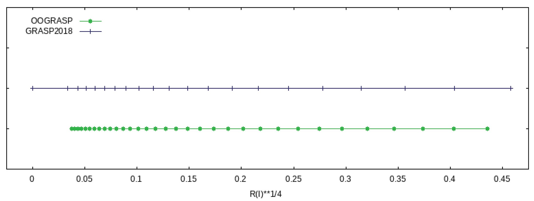
Figure 1 shows the different distributions near the origin for these two grids. This is the critical region. Plotted is every tenth point of the grid as a function of , so that is on the graph and the region near the origin is expanded somewhat. The main difference appears to be that the fully exponential grid has smaller step-sizes over the entire region, although the earlier GRASP grid has on the grid and the first non-zero value closer to the origin.
Although the exponential transformation transforms the range of r to the range of t, we now have
The advantages of this transformation will be reported, but it should also be noted here that by choosing to be an exact binary number with only one non-zero bit, the binary arithmetic involved in generating the numerical grid can be executed exactly in many cases. We will also see that arrays of will not be needed for computing Slater integrals.
4.3. The Fermi Nucleus
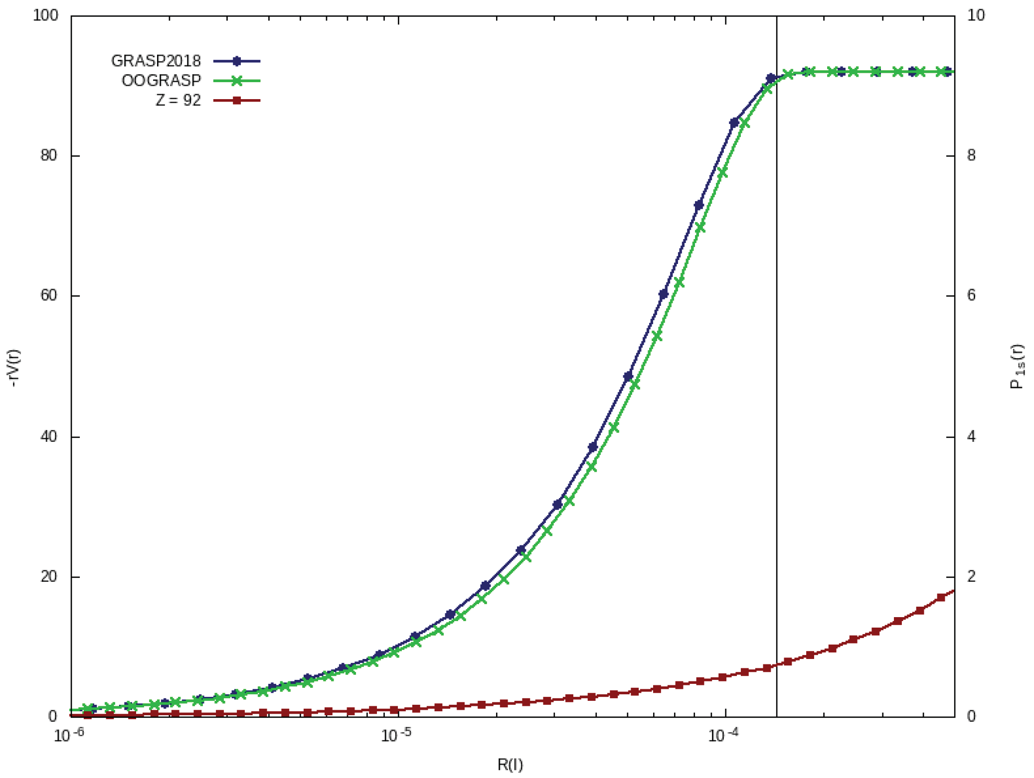
Though our numerical tests are for the point nucleus, in practice, most calculations are done for a finite nucleus such as the ’Fermi’ nucleus. Figure 2 shows the grid in the region of the origin for a uranium atom for both GRASP and present methods. The orbital for a point nucleus in the same region is also shown. Note that electrons penetrate the nucleus.
5. Simple Quadrature
An example of straightforward integrations are the normalization or orthogonality integrals, such as
Because our transformation started with the small radius , the range of integration cannot be dealt with in the t variable. Ideally, this contribution should be dealt with from a series approximation of the integrand. However, in many cases, the contribution is negligible, so our initial approach has been to ignore this contribution but monitor the error, which is easily deduced if the answer should be either unity or zero as in orthonormalization. Table 1 shows quadrature results for overlap integrals. Orthonormality results are excellent with about an extra digit of accuracy compared with GRASP2018.
6. The One-Electron Integral
A more challenging integral is the calculation of the orbital energy. By multiplying the DHF Equation (5) by the row vector and integrating, it can be shown that the orbital energy is equal to the integral referred to as [15]. The general form consists of four different integrals
where, for a point nucleus .
This formula requires the evaluation of the derivative of a function. For a numerical grid of equally spaced points, the derivative could be approximated using Stirling’s formula for seven (7) adjacent grid points, three on each side,
This symmetric formula is based on seven grid-points, whereas GRASP used a 13-point formula but with a different transformation.
Table 2 shows some non-relativistic numerical results for hydrogenic orbitals in calculations where the speed of light was . In this table, present results are compared with those reported by GRASP and the B-spline Dirac–Hartree–Fock program, DBSR-HF [20]. Generally, the present procedures are more accurate than those of GRASP, but both are less accurate for the first few integrals. In using a larger value for c than the physical speed of light, the value of the function . Any error in the calculation of Equation (13) will then be multiplied by the large value of c, resulting in larger than usual errors. With , the relativistic integrals are so small that only the non-relativistic integral is of importance and the error is in Equation (15).
7. Potential Functions
In variational methods, the energy is expressed in terms of Slater integrals which contribute to the potential functions in terms of functions , defined as follows:
where According to this definition, the calculation of functions requires the integration of integrands with factors or , where for f-electrons For large k, the finite difference approximation may not be sufficiently accurate when approximated by polynomials of lower degree.
Because functions occur frequently in atomic structure calculations, it is desirable to compute them as efficiently as possible. Hartree was developing equations with exchange when Fock published his paper and thus was pre-empted. However, Hartree was also trying to find efficient methods for computing these functions using mechanical calculators before publishing his equations. These methods are computationally the most efficient and stable methods today.
Hartree showed that the and functions are solutions of a pair of first-order equations, namely
The first equation can be integrated outward, the second inward. Transforming to the variable and multiplying by r, we obtain
with boundary conditions and , respectively.
It was shown by Worsley [23] that these equations have simple integrating factors, namely, and , respectively. On integrating, we get the equations
For our grid, since we have , parts of the calculations simplify and are essentially exact at the binary level. At the same time, if we also introduce the variable s such that , then these simplify the equations some more, namely
Both require an integration over m intervals, where m is arbitrary. For the first non-zero interval , a formula for can be used since, in terms of the r variable, the grid-points are very close together and a low order approximation may be sufficient. Thereafter, the ATSP package [24] uses along with the Simpson’s rule with an error and can be improved (after the value at has been computed) with the consequence that the errors on the odd grid points are different from the error at the even grid point.
This algorithm for solving for is stable for in that, as the integration proceeds, the error is reduced by the integration factor. The most sensitive case is . For this value of k, the calculation at large r is an othonormality integral, so that for and 0 otherwise. Thus, numerical errors are readily detected. The non-relativistic ATSP [24] package corrected the values, since in this case, the error for large values of r is easy to determine from the last few values. In relativistic calculations, with much closer to the nucleus than in ATSP, this correction was no longer needed.
For integrating these equations over two intervals, a five-point rule was used, namely,
Notice that some points outside the intervals of integration improve the polynomial approximation over Simpson’s rule.
8. Slater Integrals
The Slater integrals are defined as
where . Certain symmetries have special notations: and . Symmetry rules apply: for example .
In many applications, such as configuration interaction, numerous Slater integrals are needed and often used many times, especially in large calculations. One effective strategy is to generate lists of all possible Slater integrals for a given orbital set in a canonical form that takes into account all possible symmetries, and evaluate all integrals in advance. This is particularly effective in parallel runs, since the task can easily be distributed among the processors.
In our present object-oriented approach, lists of integrals are ordered by k. Let orbitals be ordered and let be the position of orbital a in the list consisting of orbitals. GRASP generates values of Slater integrals effectively “on demand”. A more efficient algorithm would be:
For i_a =1, n_orb
For i_c = i_a, n_orb
Compute Y^k(ac; r)
For i_b = i_a, n_orb
For i_d = I_c, n_orb
Compute and store R^k(ab,cd) integrals
The current practice in GRASP is to compute each integral using only integration which requires the generation of factors, if not already computed. With orbitals up to , k may be as large as 12. Such factors are not needed for differential equation methods, making the differential equation method more efficient computationally.
8.1. Accuracy of Slater Integrals
To our knowledge, there has been no effort made to evaluate the accuracy of Slater integrals for the relativistic hydrogenic, point nucleus case, where exact orbitals are available.
In non-relativistic theory, Slater integrals are rational numbers. By increasing the speed of light to , calculations were performed that are essentially non-relativistic. Table 4 shows the accuracy of some such integrals that we refer to as non-relativistic. The integrals are all for , although the integrals also include . The most accurate results are the B-spline results from DBSR-HF, by 2–3 digits over present finite difference methods, which in turn have about 2 more significant digits over GRASP. It has not been investigated whether the latter is the result of the binary arithmetic related to the grid and the calculations of , or the finite difference formulas used. In the present implementation, the tabulation of arrays of was not needed.
A piecewise polynomial approximation is based on a grid in which a function is approximated by a polynomial of degree in each interval between grid points. In addition, the appoximation and its first derivatives are continuous at interior grid points. Thus, the accuracy of spline approximations depend on two parameters, and the grid. In DBSR-HF, the transformation of its grid is not needed and Gaussian quadrature is used to integrate polynomials of degree less that exactly. Typically, equally spaced grid parameters are needed near the origin, followed by an exponential grid. By increasing the order of the piecewise polynomial approximation by three orders and halving the grid parameters, we obtained results that for the present purpose are “exact”.
Table 5 compares the numerical accuracy of present algorithms with those of GRASP and DBSR-HF using splines of order 9 (the default accuracy). All calculations are for the hydrogenic atom with . The “exact” values are computed using splines of order 12 and a step-size that is half the default value. We assume that the latter is exact. It is noticed that present values are considerably more accurate than those of GRASP, such as , and occasionally even more accurate than the default DBSR-HF values as for . It appears that the default DBSR-HF grid needs to be refined near the origin, particularly for s-orbitals.
However, Table 5 also draws attention to integrals with a higher value of k. For these cases, the integrand over an interval (see Equation (17)) has a factor , increasing the degree of the approximating factor for a given pair of orbitals, requiring a higher-order formula. With B-splines, it is easy to increase the order of the B-spline so that integrands of higher-order can be evaluated exactly.
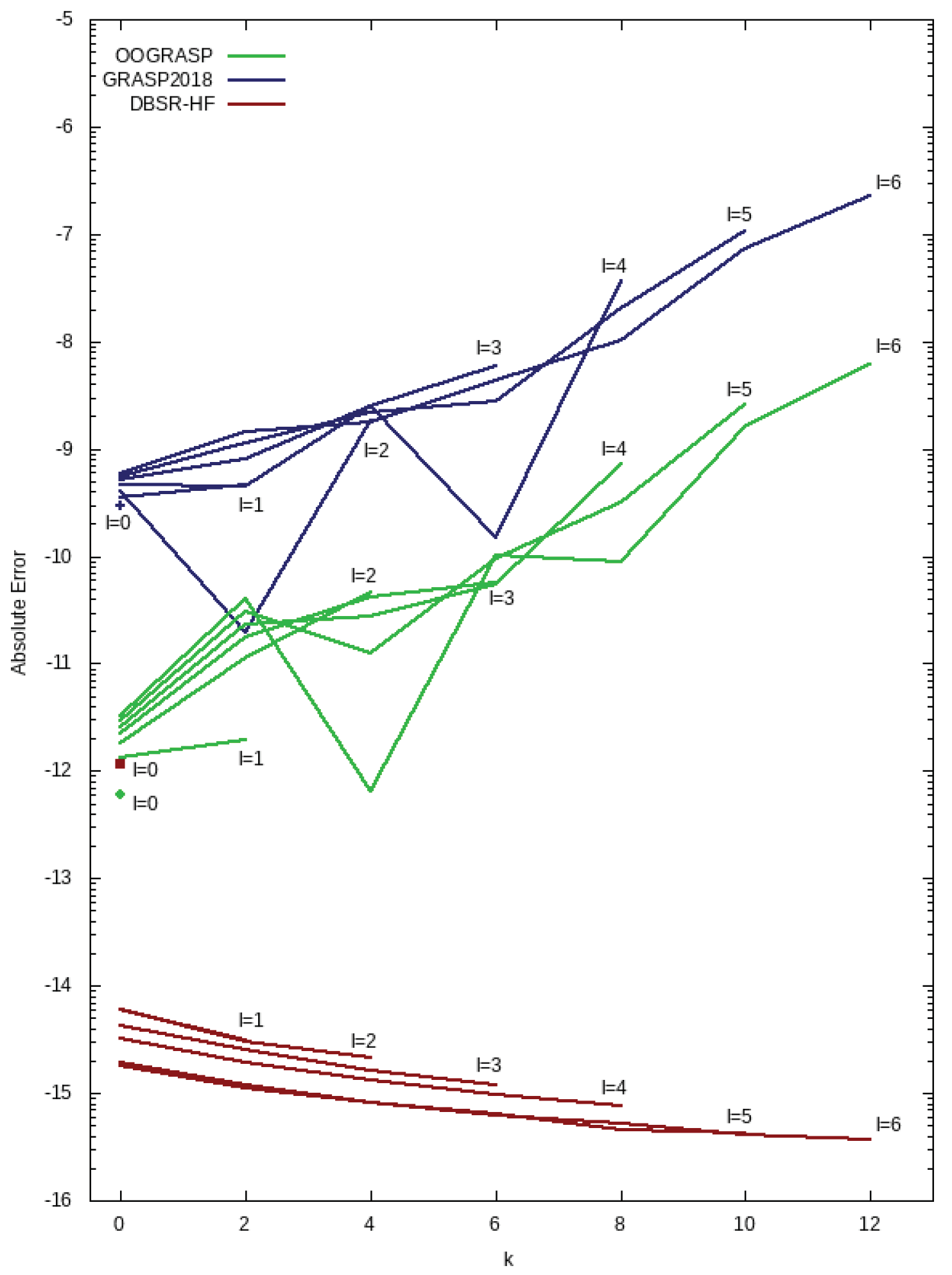
Figure 3 compares the accuracy of present, GRASP, and DBSR-HF values from the standard default order () with higher-order ”exact” values. Clearly, the DBSR-HF results are the most accurate. For the point nucleus and the r-grid with default step-size (), is a point of singularity and results can be improved to double-precision accuracy of 15–16 decimal digits by decreasing the step-size near the origin. This is particularly true for () orbital and explains the increase in accuracy as l increases. Notice the excellent accuracy as l increases for all k. However, GRASP and present results have larger errors as k increases. GRASP expresses both and in terms of integrals and powers of or evaluated using five-point formulas and a final quadrature also based on a five-point formula. Present procedures integrate the differential equations over two intervals using a five-point symmetric formula and an exponential grid as explained earlier. The final integration of Equation (27) is computed using Simpson’s rule, a three-point formula. Clearly, the error increases with l for both implementations, but the present method is more accurate by about two extra digits. These are deemed sufficiently accurate for current applications, but seven (7) point formulas for integrating the differential equations should reduce the increase with respect to l and k. Alternatively, formulas could be developed for integrating functions that have a weighting factor .
8.2. Timing
Accuracy often comes at the cost of more computational effort. As a final check, we computed the average time needed for calculating a Slater integral by running the code for numerous integrals. Table 6 shows our timing results on a standard, serial computer. It shows that the B-spline methods, though accurate to almost 16 digits, have times best measured in milliseconds, whereas both GRASP and present methods compute Slater integrals in microseconds ().
9. Solution of the DHF Equations
Since DHF equations are non-linear (the potential, for example, depends on the radial functions being computed), the equations are generally solved iteratively until results are converged or ”self-consistent”. Thus, generally, estimates of the solution are always available. Including corrections from a previous iteration will be referred to as a deferred correction.
Equation (5) expressed DHF equations as a non-linear integro-differential equation of eigenvalue type. Separating out the contribution to the potential and including this on the right-hand side simply as , we obtain a nonhomogenous equation which, for , has the form,
where, is a two component vector and
In the r variable, , the identity matrix, but in the transformed form the diagonal elements are . The function , where the latter term takes into account the effect of the finite nucleus, although it is omitted in the present study of numerical accuracy. In this form, it has been assumed that there are no off-diagonal Lagrange multipliers and the factor c for the derivative has been retained as in Ref [15]. Note also that both and decay exponentially for large r.
In many numerical methods for differential equations, the derivative would be replaced by expressions in terms of finite differences on the grid and equations established that the solution needs to satisfy. In this work, the equation is integrated and integrals are approximated by expressions in terms of values of the unknown on a grid.
Consider the simple equation with the boundary condition . The solution can be expressed as
Needed is an approximation for the integral. In this work, we will use Simpson’s rule with a correction, namely
In the DHF equations, the function is replaced by , so that the unknown quantities also appear in the integral. This is accounted for in the terms that comprise Simpson’s rule, but the correction becomes a deferred correction, computed from an estimate of the solution. The differential equation is then replaced by a set of linear equations with a three-term formula. Equation (30) applied at the midpoint of the interval, , and boundary conditions at and , leads to equations in unknowns.
In the solution proposed here, the equation at is obtained by integrating from on an exponential grid, namely
where the function
In the latter, the orbital energy is assumed to be positive. The matrices evaluated at a grid point i are denoted as , , and respectively and the 2-component vectors are . It is also useful to define the matrix
where c is a constant representing the speed of light.
9.1. Outward Integration
GRASP integrates outward over a single interval at a time, using the mid-point rule with higher-order corrections deferred (computed from previous estimates in the SCF process). In this work, integration is done over two intervals so that the highly accurate Simpson’s rule can be used for computing the new values of in terms of the previous values for . A higher-order deferred correction can be included when necessary, as done in ATSP [24].
Expressing each of the integrals in terms of values at , then rearranging the equations so that the unknown values at are defined in terms of the previous values , we obtain the three-term relationship,
which requires that and are either zero or known. In essence, the equations are systems of equations where all entries are matrices and the solution is an array of 2-component vectors.
For the DHF equations, the matrices arise from using Simpson’s rule are
The R-array includes three contributions.
- The integration of the function. Since this contribution is computed entirely in terms of functions that are already known, a five-point integration procedure can be applied directly.
- The deferred correction for the function .
- The deferred correction for the function. Note that, since , the integration of with respect to t is not exact.
When solutions are known at and i, the solution at is predicted as
The process is stable in that near the origin. Outward integration is terminated when
9.2. Near the Origin
The boundary conditions for the radial equations require that and be zero at the origin and infinity. It is customary to analyze the behavior of the solutions near the origin in terms of power series expansions [15] in r. The results depend significantly on whether the nucleus is a point nucleus or finite nucleus and also on .
In the present work, the first grid point is not at the origin. Instead of applying a different analysis depending on whether or not there is a singularity at , we could make the assumption that the differential equation at needs to be satisfied. Then,
Since DHF equations are solved iteratively, estimates are always available. Often, these are from analytic expressions for hydrogenic orbital, using the program Dirac–Coulomb wave function program DCWF [22].
9.3. Inward Integration
Outward integration may become numerically unstable in the outer tail region. At the same time, for the homogeneous equation, solutions satisfying both boundary conditions only exist for discrete eigenvalues, so part of the numerical problem is to also find these eigenvalues.
Inward integration is similar to outward integration, the only difference being that unknown values are at the point rather than . However, the problem of deciding where inward integration should start can be avoided by treating the equations in the tail region as a system of linear equations. Then, the matrix form of LU factorization can be used, that assures that the two regions join at a point, and asymptotic boundary conditions can be applied to determine whether solutions from L-factorization are satisfactorily small. When such a point has been reached, backward substitution can be applied.
The situation is somewhat different in the case of the three-term relation, in that the equation in the outward region at predicts , whereas the first equation in the tail region , uses the same value for , but also computes values . Thus, there will be differences in both components at that can be used to determine changes to the energy. Alternatively, given estimates of the radial functions, a new energy can be computed so that radial functions and orbital energies are determined iteratively.
9.4. DHF Equations as a System of Linear Equations
Let us introduce some matrices,
and define equation i as the equation for integrating over the interval Then,
or
where
and includes other corrections, including exchange and the deferred corrections. As , these matrices become constant (see Equation (29)).
At the join, is known. Values at , where M is such with for j+ i > M need to be computed. Then, the first equation for the system of equations for the unknown variables is
(since is known) and those for
Applying a matrix form of LU decomposition, we eliminate from the next equation by computing and subtracting a multiple of the equation for from i’th equation to obtain
Given the matrix, the inverse can readily be computed. When
where . The LU decomposition transforms the tridiagonal system of equations to the upper diagonal form of
To be determined is the last value of i.
In the region for large r the matrices are approaching a constant value. The last equation for which the variable has been omitted is of the form
In the exponential region, both large and small components decay exponentially so that , for example. Using this information, Equation i can be used to estimate the solution . If is sufficiently small, the equation defines M, the largest non-zero value and backward substitution determines the solution in the tail region.
For a homogeneous equation, the join may not be perfect because was not the desired eigenvalue.
9.5. The Lagrange Multipliers
So far, we have not considered the energy parameters that enter into the DHF equations because of orthogonality constraints to other orbitals with the same value of . Let the orbital under consideration be and let another orbital of the same symmetry. Then, the DHF equations have the form
Notice that, this form differs from Equation (5), in that the equations have been divided by the generalized occcupation number and include factors of r needed for the t variable. As a result of the divide, the matrix of energy parameters is no longer symmetric when , whereas the original matrix of Lagrange multiplier is symmetric. Multiplying the equation by and integrating, defines . Notice that the differentiation of orbital is required. In fact, the discussed earlier is such an integral for the one-electron orbital energy.
The variational method requires that the total energy be stationary for all variations that satisfy the boundary conditions. The off-diagonal energy parameters are associated with orbital transformations that are orbital “rotations” [1]. When two orbital subshells are both filled, such rotations change neither the wave function nor the energy, but the ”best” solution is one where , in that each orbital has one exponential tail. There are others, like , where the off-diagonal energy could be set to zero, but these are special cases that can only be detected by a rotational analysis. Another case is the case of a complete expansion where the wave function is invariant under rotation. The best solutions in those cases are in terms of natural orbitals, namely orbitals from CSF expansions, such as , etc. In effect, the degrees of freedom for rotations are used to eliminate CSFs rather than setting Lagrange multipliers to zero.
9.6. Tests for Accuracy of the Hydrogenic Equation
The differential equation methods for the hydrogenic equations can readily be evaluated to the point nucleus. As for previous tests, accuracy is assessed by observing how well the method predicts solutions when provided with estimates of machine accuracy and comparing the computed results with exact results. Table 7 reports errors for some one-electron cases of Be () for several different values of . For a point nucleus, the behavior of the large radial component ([15]) is , where . Thus, it depends on .
The process is one where the estimated solution is essentially exact, and so deferred corrections can immediately be determined. The first step is to compute the orbital energy from the function which is similar to computing the I(a,a) integral that we already discussed in an earlier section. Using the computed energy and the two initial estimates, inward and outward integration is performed. The maximum difference in this solution from the initial exact function determines the error in the computed function. The deviation from unity of the normalization integral is another test. In an iterative process, the square root of this integral is used to normalize the radial functions, and the process is repeated. For the present method, only one iteration was applied.
Table 7 shows that, for the s-orbitals, the energy is computed the most accurately. There is a slight decrease in accuracy as the energy decreases and the range expands with more grid-points included in outward integration. As increases, there is a slight improvement in the energies for higher values, possibly because the omitted contribution from the is less important as increases. The accuracy of other parameters can be expected to decrease as the number of points for outward integration increases.
Most important is how these parameters compare with the current GRASP code. Table 8 compares the present methods with those of GRASP2018, based on a mid-point rule for integration along with deferred corrections. Unlike the present method where the orbital energy was obtained in the same way as the off-diagonal energy parameters, the GRASP code uses energy adjustment procedures, outward-inward integration, variational equations that define how the radial functions change as the orbital energy changes, and series expansions at the origin. In Table 8, three quantities are compared—the orbital energy associated with the new radial functions, the difference between the new radial function for the large component, and the normalization integral of the new functions. For some reason, the least accurate orbital energy is that for , which is somewhat surprising. The normalization integral for orbitals is an order of magnitude too small resulting in the large error in for the first iteration. This suggests that there might be errors in obtaining the correct starting values but all calculations terminated after three (3) iterations with only small improvements. The errors in the large component after normalization have better accuracy but are not as accurate as the present values. After three iterations, whereas for did not improve significantly with additional iterations.
10. Conclusions
New methods for performing relativistic calculations based on Dirac theory have been proposed. The three-point Simpson’s rule is shown to provide excellent results when applied to equations based on the universal exponential grid or , along with deferred corrections that are readily applied in an iterative process. For bound state solutions, the range of integration is partitioned into the outward integration range and a tail region in which a solution is obtained that maintains continuity at the join and determines the last point. The method could also be applied to obtaining continuum solutions that require only outward integration. The range of integration would now be partitioned into the exponential grid region joined with a uniform grid at large r. A solution in the latter would be obtained that maintains continuity and applies a boundary condition at the end of the uniform region. The procedure has not yet been implemented. Further studies are also needed to solve the MCDHF equations for multi-electron systems.
Author Contributions
Both authors contributed to this paper. Both authors have read and agreed to the published version of the manuscript.
Funding
The authors acknowledge support from the Canada NSERC Discovery Grant 2017-03851.
Conflicts of Interest
The authors declare no conflict of interest.
References
- Froese Fischer, C.F.; Godefroid, M.; Brage, T.; Jönsson, P.; Gaigalas, G. Advanced multiconfiguration methods for complex atoms: I. Energies and wave functions. J. Phys. B At. Mol. Opt. Phys. 2016, 49, 182004. [Google Scholar] [CrossRef] [Green Version]
- Froese Fischer, C.; Gaigalas, G.; Jönsson, P.; Bieroń, J. GRASP2018–A Fortran 95 version of the General Relativistic Atomic Structure Package. Comput. Phys. Commun. 2019, 237, 184–187. [Google Scholar] [CrossRef]
- Li, W.; Amarsi, A.M.; Papoulia, A.; Jönsson, P. Extended multiconfiguration calculations of energy levels and transition data for C I-IV. A A 2020, in press. [Google Scholar]
- Kramida, A.; Ralchenko, Y.; Reader, J.; NIST ASD Team. NIST Atomic Spectra Database (ver. 5.7.1); National Institute of Standards and Technology: Gaithersburg, MD, USA, 2019. [Google Scholar]
- Si, R.; Li, S.; Guo, X.L.; Chen, Z.B.; Brage, T.; Jönsson, P.; Wang, K.; Yan, J.; Chen, C.Y.; Zou, Y.M. Extended Calculations with spectroscopic accuracy: Energy levels and transition properties for the fluorine-like isoelectronic sequence with Z = 24 - 30. Ap. J. Suppl. Ser. 2016, 227, 16. [Google Scholar] [CrossRef] [Green Version]
- Zhang, C.Y.; Wang, K.; Godefroid, M.R.; Jönsson, P.; Si, R.; Chen, C.Y. For heavier elements, benchmarking calculations with spectroscopic accuracy of excitation energies and wavelengths in sulfur-like tungsten. Phys. Rev. A 2020, 101, 032509. [Google Scholar] [CrossRef] [Green Version]
- Gaigalas, G.; Kato, D.; Rynkun, P.; Radziute, L.; Tanaka, M. Extended Calculations of Energy Levels and Transition Rates of Nd II-IV Ions for Application to Neutron Star Mergers. Ap. J. Suppl. Ser. 2019, 240, 29. [Google Scholar] [CrossRef]
- Tang, R.; Si, R.; Fei, Z.; Fu, X.; Lu, Y.; Brage, T.; Liu, H.; Chen, C.; Ning, C. Candidate for Laser Cooling of a Negative Ion: High-Resolution Photoelectron Imaging of Th−. Phys. Rev. Lett. 2019, 123, 203002. [Google Scholar] [CrossRef]
- Si, R.; Froese Fischer, C. Electron affinities of At and its homologous elements Cl, Br, and I. Phys. Rev. A 2018, 98, 052504. [Google Scholar] [CrossRef] [Green Version]
- Leimbach, D. The electron affinity of Astatine. Nature Commun. 2020, 11, 3824. [Google Scholar] [CrossRef]
- Froese Fischer, C.; Gaigalas, G. The Effect of Correlation on Spectra of the Lanthanides: Pr3+. Atoms 2018, 6, 8. [Google Scholar] [CrossRef] [Green Version]
- Froese Fischer, C.; Gaigalas, G. Electron correlation in the Lanthanides. Phys. Rev. A 2019, 99, 032511. [Google Scholar] [CrossRef] [Green Version]
- Gamrath, S.; Godefroid, M.R.; Palmeri, P.; Quinet, P.; Wang, K. Spectral line list of potential cosmochronological interest deduced from new calculations of radiative transition rates in singly ionized thorium (Th II). Mon. Not. R. Astron. Soc. 2020, 496, 4507–4516. [Google Scholar] [CrossRef]
- Gaigalas, G.; Fritzsche, S.; Grant, I.P. Program to calculate pure angular momentum coefficients in jj-coupling. Comp. Phys. Commun. 2001, 139, 263–278. [Google Scholar] [CrossRef] [Green Version]
- Grant, I.P. Relativisitic Quantum Theory for Atoms an Molecules; Springer Science: New York, NY, USA, 2007. [Google Scholar]
- Kozlov, M.G.; Porsev, S.G.; Safronova, M.S.; Tupitsyn, I.I. CI-MBPT: A package of programs for relativistic atomic calculations based on a method combining configuration interaction and many-body perturbation theory. Comp. Phys. Commun. 2015, 195, 199–213. [Google Scholar] [CrossRef] [Green Version]
- Verdebout, S.; Rynkun, P.; Jönsson, P.; Gaigalas, G.; Froese Fischer, C.; Godefroid, M. A partitioned correlation function interaction approach for describing electron correlation in atoms. J. Phys. B At. Mol. Opt. Phys. 2013, 46, 085003. [Google Scholar] [CrossRef] [Green Version]
- Froese Fischer, C. B-splines in variational atomic structure calculations. Adv. At. Mol. Opt. Phys. 2008, 55, 235–291. [Google Scholar]
- Froese Fischer, C. A B-spline Hartree-Fock program. Comput. Phys. Commun. 2011, 182, 1315–1326. [Google Scholar] [CrossRef]
- Zatsarinny, O.; Froese Fischer, C. DBSR—A B-spline Dirac-Hartree-Fock program. Comput. Phys. Commun. 2016, 202, 287–303. [Google Scholar] [CrossRef] [Green Version]
- Froese Fischer, C. Towards B-spline Multiconfiguration Hartree-Fock Calculations. 2006, unpublished work. Available online: https://github.com/cffischer/SPMCHF (accessed on 20 November 2020).
- Parpia, F.A.; Froese Fischer, C.; Grant, I.P. GRASP92—A package for large-scale relativistic atomic structure calculations. Comput. Phys. Commun. 1996, 94, 249–271. [Google Scholar] [CrossRef]
- Worsley, B.H. The self-consistent field with exchange for Neon by FERUT program. Can. J. Phys. 1958, 36, 289–299. [Google Scholar] [CrossRef]
- Froese Fischer, C.; Tachiev, G.; Gediminas, G.; Godefroid, M.R. An MCHF atomic-structure package for large-scale calculations. Comput. Phys. Commun. 2007, 176, 559–579. [Google Scholar] [CrossRef] [Green Version]
Figure 1.
Figure showing the different distribution of the grid points plotted versus

Figure 2.
The function such that the one-electron potential for a Fermi nucleus is . is also shown in the region of the nucleus.
Figure 2.
The function such that the one-electron potential for a Fermi nucleus is . is also shown in the region of the nucleus.

Figure 3.
Figure showing the accuracy of some integrals as a function of k for orbitals . All results are hydrogenic results.
Figure 3.
Figure showing the accuracy of some integrals as a function of k for orbitals . All results are hydrogenic results.


Table 1.
Errors in present results for overlap integrals for hydrogenic orbitals from calculations with compared with GRASP and DBSR-HF.
Table 1.
Errors in present results for overlap integrals for hydrogenic orbitals from calculations with compared with GRASP and DBSR-HF.
| Integral | Exact | DBSR-HF | GRASP | Present |
|---|---|---|---|---|
| 1.0 | 9.0 | 4.8 | 4.0 | |
| 0.0 | 8.4 | 4.0 | 9.1 | |
| 0.0 | 8.8 | 1.9 | 1.6 | |
| 1.0 | 6.7 | 5.0 | 1.2 | |
| 0.0 | 2.3 | 1.0 | 9.3 | |
| 1.0 | 7.0 | 7.0 | 4.0 | |
| 0.0 | 1.0 | 1.0 | 1.9 | |
| 1.0 | <1.0 | 1.3 | 1.1 | |
| 1.0 | 5.6 | 9.0 | 1.1 | |
| 1.0 | <1.0 | 3.6 | 1.8 | |
| 1.0 | 2.0 | 7.1 | 1.3 |
Table 2.
The error in I results for non-relativistic hydrogenic orbitals compared with GRASP and DBSR-HF. All calculations used as the value for the speed of light.
Table 2.
The error in I results for non-relativistic hydrogenic orbitals compared with GRASP and DBSR-HF. All calculations used as the value for the speed of light.
| Integral | Exact | DBSR-HF | GRASP | Present |
|---|---|---|---|---|
| I | −1/2 | 7.0 | 6.8 | 4.1 |
| I | −1/8 | 2.1 | 1.7 | 5.1 |
| I | −1/8 | 5.0 | 1.7 | 1.5 |
| I | −1/32 | 1.9 | 1.2 | 6.4 |
| I | −1/32 | 1.2 | 7.4 | 7.0 |
| I | −1/32 | 4.0 | 1.9 | 5.6 |
| I | −1/32 | 1.7 | 5.6 | 4.9 |
Table 3.
Errors in relativistic results for integrals compared with GRASP and DBSR-HF. Bold digits are not accurate.
Table 3.
Errors in relativistic results for integrals compared with GRASP and DBSR-HF. Bold digits are not accurate.
| Exact | 0.50000665659877249 | 0.12500041602953142 |
| DBSR-HF | 0.5000066566 | 0.1250004160 |
| GRASP | 0.50000665659678079 | 0.12500041602898521 |
| present | 0.50000665659644061 | 0.12500041602893869 |
| Exact | 0.12500208018974684 | 0.12500208018974684 |
| DBSR-HF | 0.1250020802 | 0.1250020802 |
| GRASP | 0.12500208022359469 | 0.12500208018969158 |
| present | 0.12500208023605386 | 0.12500208023604717 |
Table 4.
Present errors for non-relativistic Slater integral values for hydrogenic functions compared with GRASP and DBSR-HF.
Table 4.
Present errors for non-relativistic Slater integral values for hydrogenic functions compared with GRASP and DBSR-HF.
| Exact | DBSR-HF | GRASP | Present | |
|---|---|---|---|---|
| 5/8 | 1.4 | 3.0 | 6.0 | |
| 17/81 | 1.1 | 3.4 | 3.5 | |
| 59/243 | 4.7 | 1.5 | 8.3 | |
| 77/512 | 2.6 | 9.6 | 4.5 | |
| 83/512 | 3.6 | 4.2 | 1.8 | |
| 93/512 | 8.0 | 3.5 | 1.3 | |
| 541/524288 | 5.8 | 3.9 | 2.2 | |
| 943/524288 | 2.1 | 3.2 | 1.8 | |
| 693/524288 | 7.0 | 1.0 | 5.4 | |
| 743/524288 | 4.0 | 5.7 | 3.3 | |
| 413/524288 | 1.1 | 3.1 | 1.7 | |
| 239/524288 | 4.7 | 1.6 | 8.7 | |
| 373/524288 | 2.7 | 3.5 | 2.1 | |
| 373/524288 | 1.0 | 1.8 | 9.8 | |
| 759/524288 | 6.9 | 2.2 | 1.1 | |
| 333/524288 | 5.7 | 4.6 | 2.2 | |
| 16/729 | 7.0 | 1.5 | 5.8 | |
| 112/2187 | 1.1 | 8.8 | 1.8 | |
| 45/512 | 1.5 | 1.0 | 1.1 |
Table 5.
Errors in present Slater integral values for hydrogenic functions compared with GRASP2018 and DBSR-HF. For present results, some digits in boldface are digits that differ from exact values.
Table 5.
Errors in present Slater integral values for hydrogenic functions compared with GRASP2018 and DBSR-HF. For present results, some digits in boldface are digits that differ from exact values.
| Exact | 6.2622967160088860 | 1.5068979292182503 | 1.8207399944736242 |
| DBSR-HF | 6.2622967147433801 | 1.5068979291974520 | 1.8207399944825031 |
| GRASP | 6.2622967280088844 | 1.5068979671104064 | 1.8207400082805871 |
| present | 6.2622967160446317 | 1.5068979292640066 | 1.8207399944867284 |
| Exact | 2.1040290224661473 | 2.4349417985838300 | 2.4296875273216867 |
| DBSR-HF | 2.1040290222426425 | 2.4349417985761259 | 2.4296875273144032 |
| GRASP | 2.1040290227675813 | 2.4349417924772716 | 2.4296875212322915 |
| present | 2.1040290224763729 | 2.4349417985802506 | 2.4296875273181491 |
| Exact | 0.88020634371223849 | 0.87926127834665468 | 0.45441444347770305 |
| DBSR-HF | 0.88020634372399120 | 0.87926127835842560 | 0.45441444351452587 |
| GRASP | 0.88020632506820828 | 0.87926125969705382 | 0.45441444382249913 |
| present | 0.88020634369349271 | 0.87926127832752921 | 0.45441444336440395 |
| Exact | 0.51251451074058352 | 0.51158529903821337 | 0.87981921931014129 |
| DBSR-HF | 0.51251451082747790 | 0.51158529912495199 | 0.87981921934851315 |
| GRASP | 0.51251451417064353 | 0.51158530246706191 | 0.87981925908416725 |
| present | 0.51251451047002128 | 0.51158529876769843 | 0.87981922021096048 |
| Exact | 0.18323542538771756 | 0.87888382191326475 | 1.2300618797528863 |
| DBSR-HF | 0.18323542537477636 | 0.87888382192502246 | 1.2300618799962216 |
| GRASP | 0.18323541372949551 | 0.87888380326968440 | 1.2300618533910792 |
| present | 0.18323542538541401 | 0.87888382189428438 | 1.2300618797110275 |
Table 6.
Performance comparison of the average computer time () required for calculating a Slater integal for three algorithms as a function of the gfortan compiler optimization, or .
Table 6.
Performance comparison of the average computer time () required for calculating a Slater integal for three algorithms as a function of the gfortan compiler optimization, or .
| Code | ||
|---|---|---|
| DBSR-HF | 32,000 | 32,000 |
| GRASP | 2.67 | 1.85 |
| present | 2.34 | 1.48 |
Table 7.
Results showing the accuracy of the one-electron equation for from the results based on Simpson’s rule. Shown are the absolute errors in the orbital energy computed from the ”exact” wave functions (), the maximum change in the computed radial function () before normalization, the error in the normalization integral () for the solution of the differential equations, the location of the join () of outward and inward integration, the range of the solution () and difference in the large component at the join ().
| 1s | 8.0017047697086756 | 3.63 | 8.68 | 8.77 | 453 | 544 | 2.47 |
| 3s | 0.88907830376005803 | 3.14 | 9.35 | −4.67 | 524 | 585 | 2.16 |
| 5s | 0.32004636601627234 | 2.09 | 3.39 | 1.36 | 558 | 608 | 4.64 |
| 2p- | 2.0005327518841560 | 7.40 | 7.47 | −2.69 | 498 | 569 | −2.59 |
| 4p- | 0.50008656555006847 | 9.02 | 1.02 | 3.68 | 543 | 596 | −1.34 |
| 2p | 2.0001065140624612 | 9.08 | 7.49 | 1.34 | 498 | 569 | 3.11 |
| 4p | 0.50003328582209594 | 4.36 | 6.11 | 2.66 | 543 | 596 | 5.92 |
| 3d- | 0.88895200883114178 | 8.94 | 7.22 | 1.36 | 524 | 583 | −9.62 |
| 3d | 0.88890992745970487 | 2.80 | 8.88 | 2.72 | 524 | 584 | 2.75 |
Table 8.
Comparison of present methods with the mid-point methods used by GRASP2018.
| Present | GRASP | Present | GRASP | Present | GRASP | ||
| 1s | 8.0017047697086756 | 3.63 | 3.27 | 8.68 | 3.67 | 8.77 | 8.26 |
| 3s | 0.88907830376005803 | 3.14 | 1.21 | 9.35 | 5.13 | −4.67 | 1.56 |
| 5s | 0.32004636601627234 | 2.09 | 2.62 | 3.39 | 2.75 | 1.36 | 1.85 |
| 2p- | 2.0005327518841560 | 7.40 | 9.08 | 7.47 | −1.25 | −2.69 | 9.68 |
| 4p- | 0.50008656555006847 | 9.02 | −1.84 | 1.02 | −1.37 | 3.68 | 5.60 |
| 2p | 2.0001065140624612 | 9.08 | 2.62 | 7.49 | −7.01 | 1.34 | 3.20 |
| 4p | 0.50003328582209594 | 4.36 | 1.57 | 6.11 | 1.06 | 2.66 | 3.92 |
| 3d- | 0.88895200883114178 | 8.94 | 2.80 | 7.22 | −1.12 | 1.36 | 9.60 |
| 3d | 0.88890992745970487 | 2.80 | −1.26 | 8.88 | 1.72 | 2.72 | 1.33 |
Publisher’s Note: MDPI stays neutral with regard to jurisdictional claims in published maps and institutional affiliations. |
© 2020 by the authors. Licensee MDPI, Basel, Switzerland. This article is an open access article distributed under the terms and conditions of the Creative Commons Attribution (CC BY) license (http://creativecommons.org/licenses/by/4.0/).
Share and Cite
MDPI and ACS Style
Fischer, C.F.; Senchuk, A. Numerical Procedures for Relativistic Atomic Structure Calculations. Atoms 2020, 8, 85. https://0-doi-org.brum.beds.ac.uk/10.3390/atoms8040085
AMA Style
Fischer CF, Senchuk A. Numerical Procedures for Relativistic Atomic Structure Calculations. Atoms. 2020; 8(4):85. https://0-doi-org.brum.beds.ac.uk/10.3390/atoms8040085
Chicago/Turabian StyleFischer, Charlotte Froese, and Andrew Senchuk. 2020. "Numerical Procedures for Relativistic Atomic Structure Calculations" Atoms 8, no. 4: 85. https://0-doi-org.brum.beds.ac.uk/10.3390/atoms8040085
Note that from the first issue of 2016, this journal uses article numbers instead of page numbers. See further details here.