Calculation of the Differential Breit–Rosenthal Effect in the 6s6p 3P1,2 States of Hg


Department of Physics, Norwegian University of Science and Technology, NO-7491 Trondheim, Norway
*
Author to whom correspondence should be addressed.
†
This work is based on the Master thesis of the first author.
Atoms 2020, 8(4), 86; https://0-doi-org.brum.beds.ac.uk/10.3390/atoms8040086
Submission received: 19 October 2020
/
Revised: 19 November 2020
/
Accepted: 24 November 2020
/
Published: 27 November 2020
Abstract
:Studies of the hyperfine anomaly has found a renewed interest with the recent development of techniques to study the properties of long chains of unstable nuclei. By using the hyperfine structure for determining the nuclear magnetic dipole moments, the hyperfine anomaly puts a limit to the accuracy. In this paper, the differential Breit–Rosenthal effect is calculated for the states in as a function of the change in nuclear radii, using the MCDHF code, GRASP2018. The differential Breit–Rosenthal effect was found to be of the order of , in most cases much less than the Bohr-Weisskopf effect. The results also indicate that large calculations might not be necessary, with the present accuracy of the experimental values for the hyperfine anomaly.
1. Introduction
Nuclear magnetic moments carry information which allows us to draw conclusions on the basic structure of the nucleus. In that respect, they are important for basic nuclear studies, as well as for several applied sciences based on atomic physics, chemistry, and solid state physics. The electric quadrupole moment is related to the shape of the nuclear charge distribution, while the magnetic dipole moment is related to the way the nucleus carries the angular momentum. Over the years different techniques have been developed to obtain experimental values of the nuclear moments for both stable and unstable nuclei [1]. For determining the magnetic dipole moment, many of these methods require corrections for the effect of the medium upon an applied magnetic field, such as diamagnetism and Knight shift and for the non-point-like nature of the nucleus, hyperfine anomaly (HFA) [2,3]. This puts a limit on the uncertainty of the experimental values. In this work we consider corrections due to the non-point-like nature of the nucleus, the hyperfine anomaly.
The hyperfine anomaly, , is normally defined as
where one compares the ratio of the measured hyperfine structure constants for two isotopes with the independently measured ratio of the nuclear magnetic dipole moments and I, the nuclear spin for the isotopes 1 and 2. For electrons with a total angular momentum j>1/2 the anomalies to the first order may be disregarded as the corresponding wavefunctions vanish at the nucleus and are thus not affected by the extended nucleus [2,3]. However, higher-order electronic correlations may mix wavefunctions and thus lead to large anomalies in some cases, as have been observed in states [3] and in Eu [4].
The hyperfine anomaly consists of two parts, one part due to the distribution of magnetization in the nucleus, the Bohr-Weisskopf effect (BW-effect) [2,5,6] and the other due to the extended charge distribution of the nucleus, the Breit–Rosenthal effect (BR-effect) [7,8,9,10].
The influence of the finite size of the nucleus, i.e. distribution of magnetization, on the hyperfine structure was considered by Bohr and Weisskopf [5]. They calculated the hyperfine interaction (hfi) of and electrons in the field of an extended nucleus, and showed that the magnetic dipole hyperfine interaction constant (A) for an extended nucleus is generally smaller than that expected for a point nucleus. The hyperfine interaction constant is thus written as:
where is the BW-effect and the hyperfine interaction constant for a point-like nucleus.
The BR-effect, caused by the extended charge distribution [7,8,9,10], can attain values of up to 25% in absolute value. Adding this we can express the hyperfine interaction constant (A) as:
As we are not interested in the absolute values of the BW- or BR-effect but rather the differential effect and compare isotopes of an element we can write the HFA as:
In this case, we are interested in the effect of the differential BR-effect and what limits this places on the determination of the magnetic dipole moment by comparisons of the hyperfine interaction constant of different isotopes. Even if the differential BR-effect or BR-anomaly () is considered to be small, on the order of between isotope pairs, the determination of long chains of isotopes may include relatively large changes in nuclear charge distribution, especially at shape transitions, something that makes systematic studies of the differential BR-effect important.
Since the HFA has not attained much attention except in the last two decades and BR-effect even less, there has not been performed any systematic studies of the BR-effect since Rosenberg and Stroke’s paper [10] in 1972. They calculated the BR-effect using diffuse and Hofstadter-type charge distribution for isotope pairs () in several elements. In our case we are more interested in coupling the BR-anomaly () to the change in charge radius () in order to be able to use it over a long chain of isotopes. The form we would like to express the BR-anomaly is:
where the change in charge radius can be found in tables [11] or from isotope shift studies. Hg is one of the best studied examples of HFA and the experimental data provides a comparison. In addition, the BR-anomaly is also expected to be more important in corrections for heavier elements why this study may be of importance. The aim of this study is two-fold. First we want to calculate the BR-anomaly in the states in Hg as a function of the changes in nuclear charge radius. Second we want to investigate the effect of extending the configuration expansion in Multi Configurational Dirac-Hartree-Fock (MCDHF) calculations on the BR-anomaly, more specifically comparing a minimal expansion with a larger expansion. This will give an indication on how large expansions one needs to use.
2. MCDHF Method
The Multi Configurational Dirac-Hartree-Fock package (GRASP2018 [12]) used for the computations is based on the MCDHF and Relativistic Configuration Interaction (RCI) methods [13,14]. In the MCDHF approximation, atomic state functions (ASFs) are given as linear combinations of symmetry adapted configuration state functions (CSFs),
where J and M are the angular quantum numbers. The CSFs are built from products of one-electron Dirac orbitals. In the relativistic self-consistent field procedure both the radial parts of the Dirac orbitals and the expansion coefficients were optimized to self-consistency.
In RCI computations, the atomic wave function is expanded in CSFs and only the expansion coefficients are determined by diagonalizing the Hamiltonian matrix. The RCI method used, incorporated the transverse-photon (Breit) interaction and QED corrections: vacuum polarization and self-energy.
The spectroscopic states and of the electron configuration in Hg is of interest in this study, using the () as reference isotope. This isotope is the lightest stable isotope and often used as reference isotope for HFA [3]. The calculations were performed using the values tabulated for the nuclear radius, R = 5.4474(31) [11] and nuclear moment 0.5058855(9) [15].
Fermi Distribution
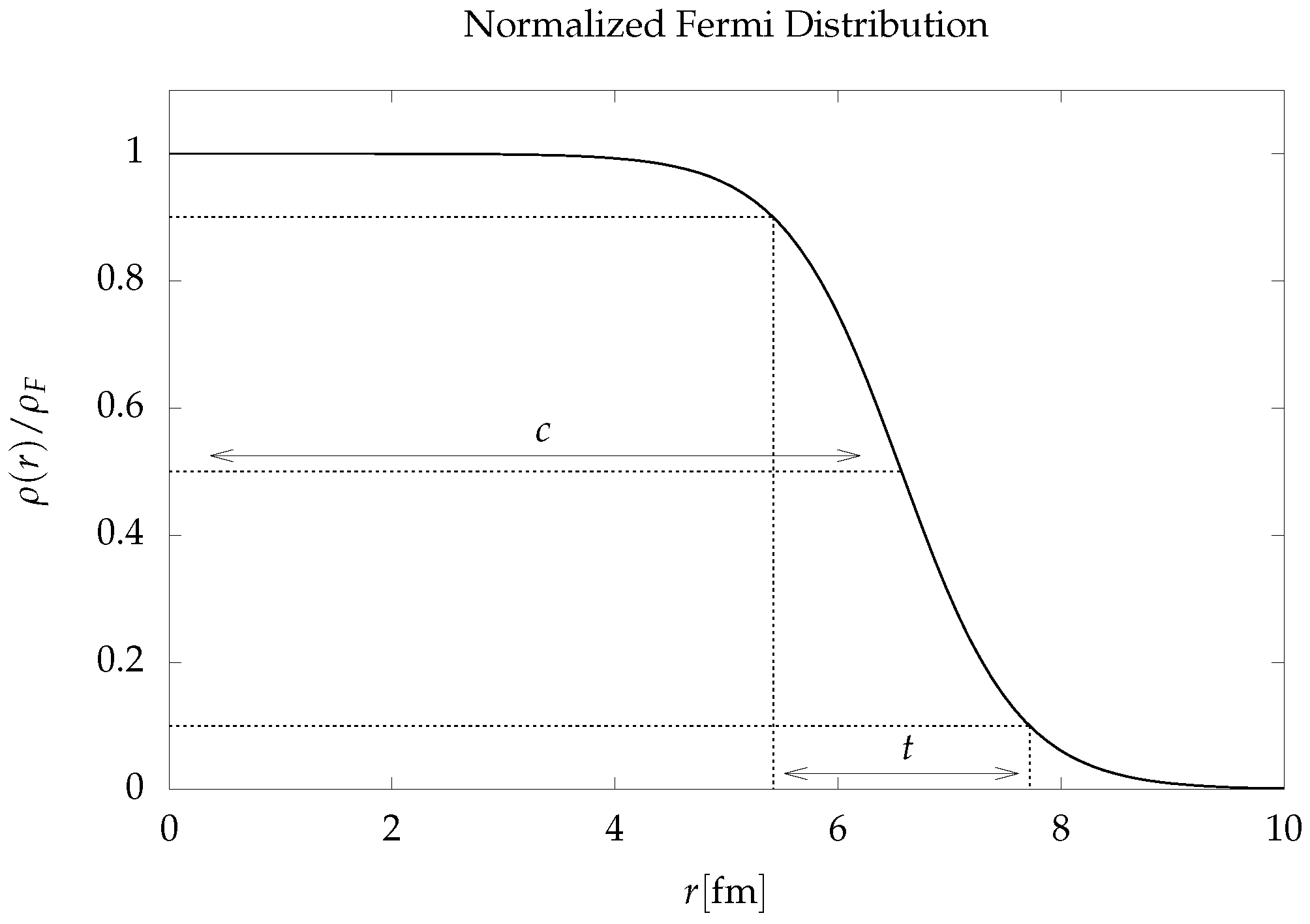
The finite charge distribution of the nucleus can be modelled in different ways with different degrees of complexity. Rosenberg and Stroke [10] used both a simple model with a homogeneous charge distribution and a Hofstadter distribution. A model, giving a realistic description, that has been used extensively is the two parameter Fermi distribution ( [16], p. 27) which also provides flexibility in calculations:
where c is the half-density radius and a is related to the so-called skin thickness t by . GRASP2018 allows for a two parameter Fermi distribution to be used to approximate the nuclear charge distribution.
Figure 1 shows the normalized Fermi distribution for the nuclear model with the rms radius 5.4474 fm from [11] and a skin thickness t = 2.3 fm [17].
The shape of the nuclear distribution can be described by the moments of the distribution. This also implies that the changes in nuclear size may be described with . However, since the differential BR-effect is expected to be small compared with the differential BW-effect and the uncertainty in the experimental data, it should be sufficient to use the first term ().
3. Calculation Procedure
With GRASP2018 the CSF expansion can be generated by starting from a small set of CSFs corresponding to a specific spectroscopic electron configuration with a specific total angular momentum. The orbitals used to build these reference CSFs are referred to as spectroscopic orbitals. The total set of CSFs is then generated by substituting electron orbitals in CSFs of the small set with orbitals corresponding to excited electrons within constraints set by the user. Different types of substitutions are used to capture important effects on the atomic properties in question. The types of substitutions are broadly divided into the number of orbitals substituted where single and double often are the most important. The set of double substitutions are further divided into valence-valence (vv) substitutions where both substituted orbitals are valence orbitals, core-valence (cv) where one orbital is from the electron core and core-core (cc) where both substitutions are made from the electron core. Substitutions with core orbitals are used to capture core polarisation effects which could have an impact on the hyperfine interactions.
The calculations were done in two steps, first the hfs constants were calculated in gradually increased expansions until the values converged. The obtained expansion was then used to calculate the hfs constants for different nuclear radii.
3.1. Obtaining Spectroscopic Orbitals
To obtain convergence while optimizing the radial functions, we employed a similar method as used by Bieroń et al. [18] for calculations in in . That is, the spectroscopic orbitals are optimized with a small number of reference CSFs, which are kept frozen during optimization of the virtual orbitals as the set of CSFs is expanded. In calculations on similar systems such as the states in [18], and and in [19], the minimal expansions have been used for the reference and the virtual orbitals have been added and optimized in layers. A layer of virtual orbitals, referred to as a virtual layer, is a set of virtual orbitals which contains no more than one orbital with quantum number . As the radial functions of each new layer are optimized, all previously obtained functions are kept frozen.
The minimal expansion for the state included the CSFs corresponding to the relativistic configurations
For the state the minimal expansion included only the CSF corresponding to the relativistic configuration
All calculations were done separately for the two states. The radial functions for the spectroscopic orbitals were optimized simultaneously under the self consistent field (scf) procedure with the minimal expansions.
3.2. Obtaining Virtual Orbitals
The virtual orbitals were added in layers by extending the CSF expansion to include CSFs generated by substitutions from a subset of the orbitals in the reference with orbitals in the new virtual layer. Scf calculations were done where all new radial functions were optimized simultaneously while all previously optimized functions were kept frozen.
The CSF expansions were in each case generated by all single as well as double vv and cv substitutions from the core subshells and valence subshells ( and for , and for ) up to all new and previously obtained orbitals.
After the scf calculations for each new virtual layer, a relativistic configuration interaction (RCI) was done where the transverse photon interaction, vacuum polarization and self energy corrections were included. Self energy corrections were included for orbitals with principal quantum number . The CSF expansion was regenerated for the RCI where the Dirac-Coulomb-Breit operator was used for removal of non-interacting CSFs. The hfs constant was calculated after each RCI. The addition of the 4th virtual layer changed the calculated value by approximately % and % for the states and , respectively, so no further layers were added. The compositions of the 4 virtual layers and the change in the value of the hfs constant from the preceding calculation can be viewed in Table 1.
For the 1st virtual layer included both and which is an exception to the definition given for a virtual layer. The reason for this is that the orbital was not included in the minimal expansion.
3.3. Obtaining the ASF
3.3.1. Single and Core-Valence Substitutions
The subshells in the core were opened for single and cv substitutions to the 4 virtual layers. The subshells were opened one by one in the order and then . The maximum number of orbitals in the active set (virtual and open spectroscopic orbitals) that a CSF can be constructed from is limited by the program to 20. The maximum number of open relativistic core subshells is therefore 17 under the cv substitutions. In order to be able to study the effect of core subshells with , the subshells were closed as the and subshells were opened for substitutions. The and subshells were closed for a calculation where the subshells were opened. The changes in the calculated hfs constant relative to the preceding calculation as each subshell was opened are presented in Table 2.
When cc substitutions are included, the maximum number of open subshells is 16 due to the aforementioned limitation. The lowest contributing subshells with respect to the hfs constant were the , and subshells for both states. These subshells were therefore closed for substitutions in the further calculations. The contributions from each of these subshells were on the order of % or less.
The significance of the different virtual orbitals were estimated by calculating the hfs constant for sets of CSFs generated by single, vv and cv substitutions from the subshells to different subsets of the virtual orbitals. The smallest subset consisted of the virtual orbitals with and . The set was extended by allowing substitutions up to one new orbital symmetry at a time in the order , , , and finally . The relative changes from the preceding calculations are presented in Table 3.
The orbitals were omitted from the active set in the further calculations for due to the very low contribution. Contributions from virtual orbitals not included are expected to be small from the trend of decreasing contributions with increasing principal and orbital quantum numbers. The resulting approximations then became the expansions generated by single, vv and cv substitutions from the subshells to the virtual orbitals , which contained 65,443 and 62,211 CSFs for the states and , respectively.
3.3.2. Core-Core Substitutions
The CSF expansions from the approximations with single, vv and cv substitutions were extended further with cc substitutions. Double substitutions were first allowed from the core subshells to the active set where virtual orbitals with and were included. Virtual orbitals were then included in the order then etc. The relative changes from the preceding calculations are presented in Table 4.
The CSFs generated by cc substitutions from to were kept for , and those from to were kept for along with the final expansions with the single, vv and cv approximations as the CSF expansion was extended further by including cc substitutions from the subshells . The virtual orbital was dropped for the state due to the low contribution. All CSFs generated up to this point were kept as the expansion was extended further using cc substitutions from lower core subshells.
The number of CSFs grows rapidly with inclusion of cc substitutions from and so only the virtual orbitals in the 1st virtual layer, as defined in Table 1, were included in the first calculation. This reduced the value of the hfs constant by approximately % for and % for . When also including the subshell in the expansion the value was reduced further by approximately % for and increased by approximately % for . cc substitutions from , or any of the lower subshells, were therefore not included for the further extension of the expansion.
Orbitals of the 2nd virtual layer were included in the order and the hfs constant was calculated between each inclusion. The results are presented in Table 5.
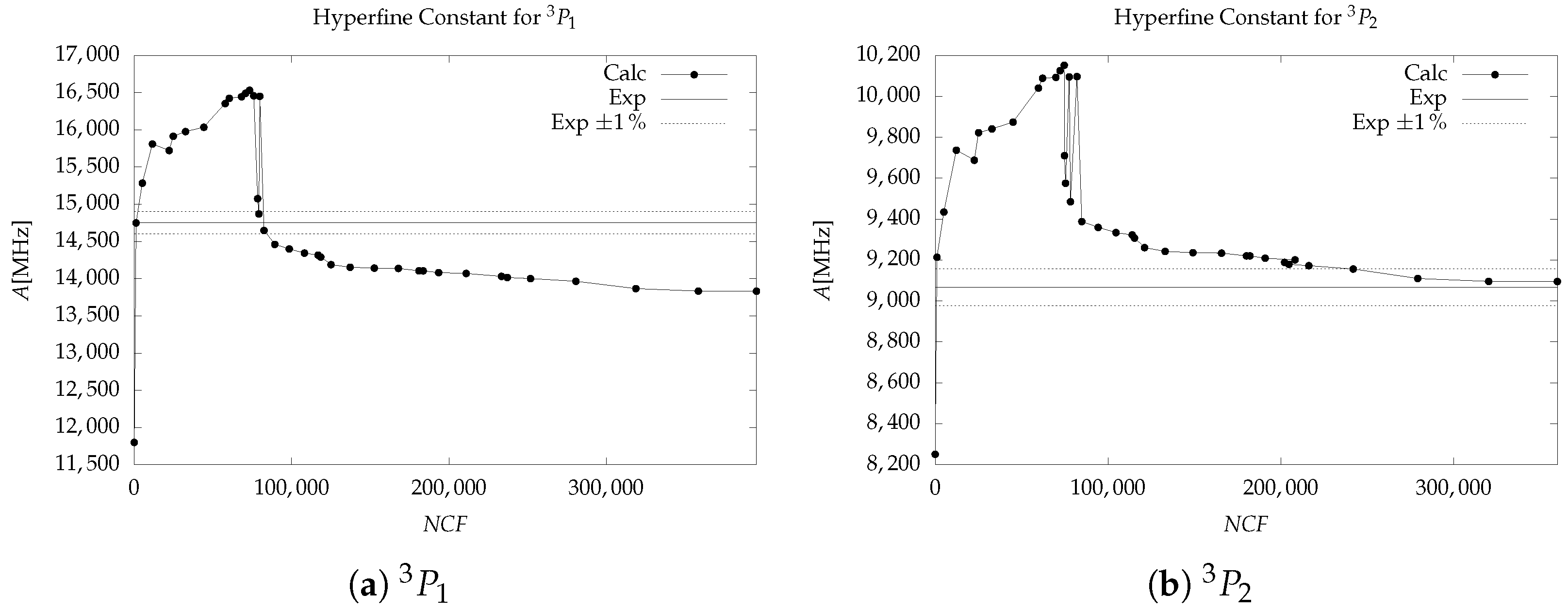
At this point the contributions from the CSFs not included in the expansion were considered to be less than a percent. The graphs in Figure 2 show the calculated values of the hfs constant as the set of CSFs was extended for each of the states. It can be seen that the use of single, vv and cv substitutions resulted in an overshooting of the hfs value while the use of cc substitutions relaxed this overshooting. The graphs show similarities with the one obtained for 201Hg by Bieroń et al. [18] except for it being reflected around the horizontal axis due to the gyromagnetic ratio of 201Hg having opposite sign. For the state the value converges within 1% of the experimental value. For the value seems to converge, but toward a value that is approximately 6% lower than the experimental value. The final expansions consisted of 395,461 CSFs for and 359,985 CSFs for . It should be noted that we have not included the BW-effect in the calculations.
3.3.3. Variations in Nuclear Radius
The nuclear radius of Hg isotopes (and isomers) vary with a substantial odd-even staggering. In order to address this we performed calculations with changes in the mean squared radius of . Using the final CSF expansions obtained for 199Hg, all radial functions and expansion coefficients were recalculated for the ASFs for both states with values of the nuclear mean squared radius at increments of . The nuclear skin thickness was first kept constant.
For the state , we made a series of calculations where the skin thickness was varied in steps of . These values correspond to 1 and 2 standard deviations of the experimental skin thickness from scattering experiments [16]. This range was considered to be a conservative estimate of how much the nuclear skin thickness is expected to differ from the standard value for the Hg isotopes.
4. Results
The results of the calculations of different nuclear radii with the large CSF expansion are presented in Table 6 and Figure 3 and with the the minimal CSF expansions presented in Table 7. For each state and expansion, we obtain the proportionality constants (Table 8).
It is apparent that using the minimal expansion was quite similar to that calculated with the largest expansion. The largest difference was for where the value differs by approximately % from the minimal to the largest expansion. For the value differs by approximately %. This indicates that large CSF expansions and the associated large computational efforts may not be necessary for calculation of the BR-anomaly, at least for systems only containing s- and p-electrons, unless even higher precision is needed. This can be explained by the fact that in the minimal expansions the only orbitals contributing to the magnetic hyperfine interaction are the valence orbitals since all other subshells are closed. The largest expansions include CSFs with open core subshells which contribute to the hyperfine interaction, which can be described as core polarization. The BR-anomaly is mostly dependant on the and orbitals since these are the only ones with non-zero probability densities at the nucleus which is required for the first order corrections to the BR correction. The small difference in between the minimal and largest expansion indicates that the BR-anomaly is mostly unaffected by the principal quantum number n for the and subshells that contribute to the hyperfine interaction.
The variation in the hfs constant for different values of the skin thickness gave a minor change in the proportionality constant as can be seen in Table 9. The effect is quite small and thus not expected to be of any importance. The uncertainty in the proportionality constant can for the results be estimated to be less than 10%, why we choose this error as a conservative value.
This makes it possible to express the BR-anomaly in the and as
5. Discussion
5.1. Comparisons with Other Calculations
The systematic study by Rosenberg and Stroke [10] cannot be directly compared to our results as they calculated the s- and electron contributions to the BR-effect between isotope-pairs, their weighted value () of the contributions give the same order of magnitude as our results (). More recent work on calculating the BR-anomaly as a function of changes in the nuclear charge radius can be found in one-electron systems. In Cs(Z = 55), Gustavsson and Mårtensson-Pendrill [20] found a value of for the 6s state. Calculations in Tl (Z = 81) yielded values of and for the and electrons, respectively. Values has also been reported in Fr (Z = 87) [21], and for the and electrons, respectively. The values are on the same order as our results, albeit using more advanced methods, showing that our results are reasonable. It is also clear that even a small expansion in s- and p- electron systems gives reasonable values compared with the experimental uncertainties.
5.2. HFA in Hg and BR-Anomaly
The calculated BR-anomaly can be compared with experimental HFA to find out how important a correction due to the BR-anomaly can be. Since the BR-effect is only expected to be of major importance when the BW-effect is small, that is when the spins of the nuclei are the same [2,3], we can limit the comparison to these nuclei. In this case we have two series, the ground states and the isomer states, where the HFA has been extracted. In Table 10 the nuclei are compared using as reference and in Table 11 the nuclei are compared using as reference.
From the results, one can observe that the BR-anomaly is less than 10% of the experimental hfa in the I = 1/2 isotopes, while in the I = 13/2 isotopes up to 30% of the hfa is due to the BR-anomaly. This indicates that it would be advantageous to revisit the I = 13/2 isomers in Hg with high resolution experiments in order to further investigate the hfa in these nuclei as a way to further investigate the validity of the semi-empirical Moskowitz-Lombardi formula [23].
Recent experiments at CERN [24,25] on neutron-deficient Hg has yielded values of changes in the nuclear charge radius and nuclear magnetic moments to . In these cases, one has to correct for the HFA in order to obtain the nuclear magnetic moment. In the paper of Sels et al. [25] they employ the Mozkowitz-Lombardi semi-empirical formula [23] as a way to deduce the BW-anomaly while using the calculations of Rosenberg and Stroke [10] for estimating the BR-anomaly. Compared with our calculations, their values are too large. They report and while our results are and . This will, however, not change the values of the nuclear magnetic dipole moments as the experimental uncertainty is large.
5.3. Future Work
As we showed, at least for sp-configurations, the BR-anomaly may be calculated using relatively small expansions with the MCDHF method. This opens up for systematic calculations of the BR-anomaly in heavy elements, and the possibility to obtain values of the nuclear magnetic dipole moment with better accuracy or smaller uncertainty as discussed in the IAEA report on evaluation of nuclear moments [26]; however, our results indicate that this is only possible for isotopes with the same nuclear spin where the BW-effect is expected to be small.
Author Contributions
Conceptualization, J.R.P.; methodology, T.H. and J.R.P.; software, T.H.; validation, J.R.P.; formal analysis, T.H.; investigation, T.H. and J.R.P.; data curation, T.H. and J.R.P.; writing–original draft preparation, T.H. and J.R.P.; writing–review and editing, T.H. and J.R.P.; visualization, T.H.; supervision, J.R.P.; project administration, J.R.P. All authors have read and agreed to the published version of the manuscript.
Funding
This research received no external funding.
Conflicts of Interest
The authors declare no conflict of interest.
References
- Otten, E.W. Nuclear radii and moments of unstable isotopes. In Treatise on Heavy Ion Science; Springer: Berlin/Heidelberg, Germany, 1989; pp. 517–638. [Google Scholar]
- Büttgenbach, S. Magnetic Hyperfine Anomalies. Hyperfine Interact. 1984, 20, 1–64. [Google Scholar] [CrossRef]
- Persson, J.R. Table of hyperfine anomaly in atomic systems. At. Data Nucl. Data Tables 2013, 99, 62–68. [Google Scholar] [CrossRef] [Green Version]
- Persson, J.R. Determination of core polarization in Eu+ using the hyperfine anomaly. Phys. Scr. 2007, 76, 449–451. [Google Scholar] [CrossRef]
- Bohr, A.; Weisskopf, V. The influence of nuclear structure on the hyperfine structure of heavy elements. Phys. Rev. 1950, 77, 94. [Google Scholar] [CrossRef]
- Fujita, T.; Arima, A. Magnetic hyperfine structure of muonic and electronic atoms. Nucl. Phys. A 1975, 254, 513–541. [Google Scholar] [CrossRef]
- Rosenthal, J.E.; Breit, G. The isotope shift in hyperfine structure. Phys. Rev. 1932, 41, 459. [Google Scholar] [CrossRef]
- Crawford, M.; Schawlow, A. Electron-nuclear potential fields from hyperfine structure. Phys. Rev. 1949, 76, 1310. [Google Scholar] [CrossRef]
- Ionesco-Pallas, N. Nuclear Magnetic Moments from Hyperfine Structure Data. Phys. Rev. 1960, 117, 505. [Google Scholar] [CrossRef]
- Rosenberg, H.; Stroke, H. Effect of a diffuse nuclear charge distribution on the hyperfine-structure interaction. Phys. Rev. A 1972, 5, 1992. [Google Scholar] [CrossRef]
- Angeli, I.; Marinova, K.P. Table of experimental nuclear ground state charge radii: An update. At. Data Nucl. Data Tables 2013, 99, 69–95. [Google Scholar] [CrossRef]
- Fischer, C.F.; Gaigalas, G.; Jönsson, P.; Bieroń, J. GRASP2018—A Fortran 95 version of the general relativistic atomic structure package. Comput. Phys. Commun. 2019, 237, 184–187. [Google Scholar] [CrossRef]
- Fischer, C.F.; Godefroid, M.; Brage, T.; Jönsson, P.; Gaigalas, G. Advanced multiconfiguration methods for complex atoms: I. Energies and wave functions. J. Phys. B At. Mol. Opt. Phys. 2016, 49, 182004. [Google Scholar] [CrossRef] [Green Version]
- Grant, I.P. Relativistic Quantum Theory of Atoms and Molecules: Theory and Computation; Springer Science & Business Media: Berlin/Heidelberg, Germany, 2007; Volume 40. [Google Scholar]
- Stone, N. Table of nuclear magnetic dipole and electric quadrupole moments. At. Data Nucl. Data Tables 2005, 90, 75–176. [Google Scholar] [CrossRef]
- Elton, L.R.B. Nuclear Sizes; Oxford University Press: London, UK, 1961; Volume 561. [Google Scholar]
- Mårtensson-Pendrill, A.M. Atoms through the looking glass–a relativistic challenge. Can. J. Phys. 2008, 86, 99–109. [Google Scholar] [CrossRef] [Green Version]
- Bieroń, J.; Pyykkö, P.; Jönsson, P. Nuclear quadrupole moment of Hg 201. Phys. Rev. A 2005, 71, 012502. [Google Scholar] [CrossRef]
- Bieroń, J.; Fischer, C.F.; Indelicato, P.; Jönsson, P.; Pyykkö, P. Complete-active-space multiconfiguration Dirac-Hartree-Fock calculations of hyperfine-structure constants of the gold atom. Phys. Rev. A 2009, 79, 052502. [Google Scholar] [CrossRef] [Green Version]
- Gustavsson, M.G.; Mårtensson-Pendrill, A.M. Four decades of hyperfine anomalies. In Advances in Quantum Chemistry; Elsevier: Amsterdam, The Netherlands, 1998; Volume 30, pp. 343–360. [Google Scholar]
- Mårtensson-Pendrill, A.M. Isotopes through the looking glass. Hyperfine Interact. 2000, 127, 41–48. [Google Scholar] [CrossRef]
- Ulm, G.; Bhattacherjee, S.; Dabkiewicz, P.; Huber, G.; Kluge, H.J.; Kühl, T.; Lochmann, H.; Otten, E.W.; Wendt, K.; Ahmad, S.; et al. Isotope shift of 182 Hg and an update of nuclear moments and charge radii in the isotope range 181 Hg-206 Hg. Z. Phys. A At. Nucl. 1986, 325, 247–259. [Google Scholar] [CrossRef]
- Moskowitz, P.; Lombardi, M. Distribution of nuclear magnetization in mercury isotopes. Phys. Lett. B 1973, 46, 334–336. [Google Scholar] [CrossRef]
- Marsh, B.; Goodacre, T.D.; Sels, S.; Tsunoda, Y.; Andel, B.; Andreyev, A.; Althubiti, N.; Atanasov, D.; Barzakh, A.; Billowes, J.; et al. Characterization of the shape-staggering effect in mercury nuclei. Nat. Phys. 2018, 14, 1163–1167. [Google Scholar] [CrossRef] [Green Version]
- Sels, S.; Goodacre, T.D.; Marsh, B.; Pastore, A.; Ryssens, W.; Tsunoda, Y.; Althubiti, N.; Andel, B.; Andreyev, A.; Atanasov, D.; et al. Shape staggering of midshell mercury isotopes from in-source laser spectroscopy compared with density-functional-theory and Monte Carlo shell-model calculations. Phys. Rev. C 2019, 99, 044306. [Google Scholar] [CrossRef] [Green Version]
- Stone, N.; Stuchbery, A.; Dimitriou, P. Evaluation of Nuclear Moments; Technical Report INDC(NDS)-0732; International Atomic Energy Agency: Wien, Austria, 2017; Technical Report INDC(NDS)-0732. [Google Scholar]
Figure 1.
Fermi distribution with half-density radius c and skin thickness t for the nuclear model of 199Hg.
Figure 1.
Fermi distribution with half-density radius c and skin thickness t for the nuclear model of 199Hg.

Figure 2.
Calculated values of the hyperfine constant A with increasing CSF expansions. The horizontal lines show the experimental values %.
Figure 2.
Calculated values of the hyperfine constant A with increasing CSF expansions. The horizontal lines show the experimental values %.

Figure 3.
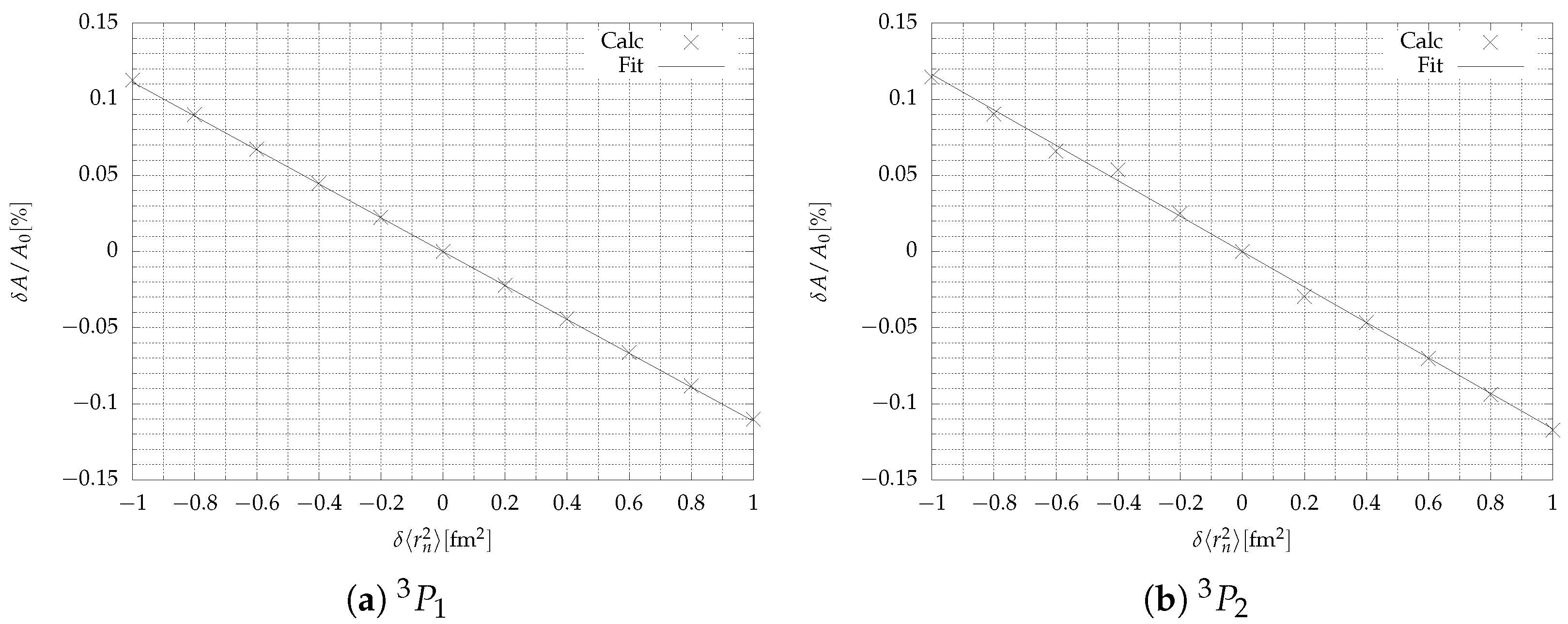
Relative change in the hyperfine structure constant with variation in the mean squared radius of the nuclear charge distribution from the reference nucleus with hyperfine structure constant in the electronic states and with the largest expansions. The solid line represents the linear fit .
Figure 3.
Relative change in the hyperfine structure constant with variation in the mean squared radius of the nuclear charge distribution from the reference nucleus with hyperfine structure constant in the electronic states and with the largest expansions. The solid line represents the linear fit .


Table 1.
Orbitals included in the different virtual layers. The parentheses around orbital indicates that it was included only for the state. is the relative change in the hyperfine structure constant from the preceding calculation.
Table 1.
Orbitals included in the different virtual layers. The parentheses around orbital indicates that it was included only for the state. is the relative change in the hyperfine structure constant from the preceding calculation.
| Virtual Layer | Orbitals | ||
|---|---|---|---|
| 1st | () | 24 | 12 |
| 2nd | |||
| 3rd | |||
| 4th |
Table 2.
Relative change from the preceding calculation in the value of the hyperfine structure constant as the core subshells were opened for single, vv and cv substitutions.
Table 2.
Relative change from the preceding calculation in the value of the hyperfine structure constant as the core subshells were opened for single, vv and cv substitutions.
| Subshell | ||
|---|---|---|
Table 3.
Relative change in the hyperfine structure constant A from the preceding calculation as the virtual orbitals were included in the order , etc. with single, vv and cv substitutions.
Table 3.
Relative change in the hyperfine structure constant A from the preceding calculation as the virtual orbitals were included in the order , etc. with single, vv and cv substitutions.
| Virtual Orbitals | ||
|---|---|---|
| 11 | ||
Table 4.
Relative changes in the hyperfine constant A from the preceding calculation as the virtual orbitals were included in the order , etc. for cc substiutions from .
Table 4.
Relative changes in the hyperfine constant A from the preceding calculation as the virtual orbitals were included in the order , etc. for cc substiutions from .
| Virtual Orbitals | ||
|---|---|---|
Table 5.
Relative changes in the hyperfine constant A from the preceding calculation as the virtual orbitals were included in the order 1st virtual layer, , , …, . for cc substiutions from .
Table 5.
Relative changes in the hyperfine constant A from the preceding calculation as the virtual orbitals were included in the order 1st virtual layer, , , …, . for cc substiutions from .
| Virtual Orbitals | ||
|---|---|---|
| 1st layer | ||
Table 6.
Relative change in the hyperfine structure constant with variation in the mean squared radius of the nuclear charge distribution from the reference nucleus with hyperfine structure constant in the electronic states and with the largest expansions.
Table 6.
Relative change in the hyperfine structure constant with variation in the mean squared radius of the nuclear charge distribution from the reference nucleus with hyperfine structure constant in the electronic states and with the largest expansions.
| 0.2 | ||
| 0.4 | ||
| 0.6 | ||
| 0.8 | ||
| 1.0 |
Table 7.
Relative change in the hyperfine structure constant with variation in the mean squared radius of the nuclear charge distribution from the reference nucleus with hyperfine structure constant in the electronic states and with the minimal expansions.
Table 7.
Relative change in the hyperfine structure constant with variation in the mean squared radius of the nuclear charge distribution from the reference nucleus with hyperfine structure constant in the electronic states and with the minimal expansions.
| 0.2 | ||
| 0.4 | ||
| 0.6 | ||
| 0.8 | ||
| 1.0 |
Table 8.
The proportionality constant (in ) for the states and with both the largest and minimal expansions.
Table 8.
The proportionality constant (in ) for the states and with both the largest and minimal expansions.
| State | Largest | Minimal |
|---|---|---|
| −0.1113 | −0.1106 | |
| −0.1164 | −0.1196 |
Table 9.
Calculated proportionality constant in the linear fit for different skin thickness deviations from the reference model ().
Table 9.
Calculated proportionality constant in the linear fit for different skin thickness deviations from the reference model ().
| [% fm] | |
|---|---|
| −0.2 | −0.1166 |
| −0.1 | −0.1167 |
| 0 | −0.1164 |
| 0.1 | −0.1157 |
| 0.2 | −0.1158 |
Table 10.
Experimental HFA for I = 1/2 isotopes compared with the BR-anomaly.
| Isotope | [22] | ||
|---|---|---|---|
| 195 | −0.067 | 0.1470(9) | 0.0156 |
| 197 | −0.139 | 0.0778(7) | 0.0075 |
Table 11.
Experimental HFA for I = 13/2 isotopes compared with the BR-anomaly.
| Isotope | [22] | ||
|---|---|---|---|
| −0.105 | 0.061 | 0.011 | |
| −0.194 | 0.078 | 0.021 | |
| −0.217 | 0.095 | 0.031 |
Publisher’s Note: MDPI stays neutral with regard to jurisdictional claims in published maps and institutional affiliations. |
© 2020 by the authors. Licensee MDPI, Basel, Switzerland. This article is an open access article distributed under the terms and conditions of the Creative Commons Attribution (CC BY) license (http://creativecommons.org/licenses/by/4.0/).
Share and Cite
MDPI and ACS Style
Heggset, T.; Persson, J.R. Calculation of the Differential Breit–Rosenthal Effect in the 6s6p 3P1,2 States of Hg. Atoms 2020, 8, 86. https://0-doi-org.brum.beds.ac.uk/10.3390/atoms8040086
AMA Style
Heggset T, Persson JR. Calculation of the Differential Breit–Rosenthal Effect in the 6s6p 3P1,2 States of Hg. Atoms. 2020; 8(4):86. https://0-doi-org.brum.beds.ac.uk/10.3390/atoms8040086
Chicago/Turabian StyleHeggset, Tarjei, and Jonas R. Persson. 2020. "Calculation of the Differential Breit–Rosenthal Effect in the 6s6p 3P1,2 States of Hg" Atoms 8, no. 4: 86. https://0-doi-org.brum.beds.ac.uk/10.3390/atoms8040086
Note that from the first issue of 2016, this journal uses article numbers instead of page numbers. See further details here.