Stark-Zeeman Broadening of Spectral Line Shapes in Magnetized Plasmas

Abstract

In this work, we studied the Lyman-alpha line in the presence of a magnetic field, such as the ones found at the edge of tokamaks. The emphasis is on the contribution of the motional Stark effect on line broadening, which may have comparable effects to the internal plasma microfields for the spectral line in question. The effect of the magnetic field, temperature, and the Maxwell distribution of the ion velocities and density on Lyman-alpha are studied.

1. Introduction

Spectroscopy is often used for non-intrusive tokamak diagnostics, as atomic parameters are modified by the surrounding plasma. Typically observed atomic properties, such as widths and shifts or level splittings are compared to calculations that account for the plasma environment, e.g., density, temperature, magnetic field, etc. Such calculations of line profiles take into account the fact that a spectral line shape is a complex function of the interaction of the emitter with perturbers and external fields as well as on the internal structure of the emitter. So far, the majority of research on line profile only accounts for the Stark effect [1]. However, magnetic fields also play an important role in a number of areas of current interests: Astrophysics (magnetic stars, white dwarfs, stars neutron), plasmas generated by high energy lasers, and magnetic fusion (tokamak, stellarator, pinch). Comparatively, little work has been done for plasmas in the presence of the magnetic field. Stark–Zeeman effects on spectral lines is still largely unexplored, with only few theoretical studies opening the way for more research [2,3,4,5].

Among these works, Nguyen-Hoe et al. [5] calculated the profiles of hydrogen lines in the presence of electron collisions, the static ion microfield, and an external uniform magnetic field. They considered electron densities between 10${}^{15}$ cm${}^{-3}$ and 10${}^{18}$ cm${}^{-3}$ and magnetic fields less than or equal to 12 tesla. Results concerning the Lyman-$\alpha$, Lyman-$\beta$, and the Lyman and Balmer $\alpha$ were obtained. For very low magnetic fields B, the profiles merge with the pure Stark profiles, previously calculated by [6,7,8].

For large $B>1$ Tesla, the line shapes deviate significantly from a pure Stark profile. These differences depend both on the orientation of the viewing direction relative to the magnetic field, and on the ratio between the displacement due to the Zeeman single magnetic field and the Stark shift due to the plasma electric microfield. The dependence on the emission angle, relative to the magnetic field, complicates the calculation because the assumption of an isotropic plasma is no longer valid in the presence of a magnetic field.

The magnetic field has a number of effects: First, it splits the atomic levels of the emitter. Second, it modifies the motion and distribution functions of the plasma particles. This has been studied in [9,10] and it was found that the spiraling motion of charged particles may be neglected if the line width is much larger than the cyclotron frequency and in addition, because of competing effects, modifications are typically not large.

In this work we focus on a third effect, the motional Stark effect and its influence on the emitter, rather than the motion of the plasma particles. Since, in intense magnetic fields, this phenomenon may be more important than the Stark effect itself and does not consider other effects.

This work is organized as follow: First, the relevant equations and parameters are introduced in Section 2. In Section 3, a version of the Stark broadening theory, including the motional Stark effect is presented. We neglect fine structure effects because of the strong magnetic fields of interest ($B>1$ Tesla). Section 4 presents the results and compares and contrasts the role of different effects in relation to line broadening. A brief conclusion follows in Section 5.

2. Motional Stark Effect (MSE)

Due to the motion of the emitter with velocity $\overrightarrow{V}$ in the magnetic field $\overrightarrow{B}$, the emitting electron experiences an electric field-called ‘Lorentz field’ in this paper, given by:

$$\overrightarrow{E_L}=\overrightarrow{V}\times \overrightarrow{B}$$

(1)

This field produces a Stark effect in the reference frame of the emitter, so that the total Hamiltonian takes the form:

$$H(E,B)=H_0+H_{sf}+\overrightarrow{d}·\overrightarrow{E}\left(t\right)+\hslash \overrightarrow{\omega }·\left(\overrightarrow{L}+2\overrightarrow{S}\right)+\overrightarrow{d}·(\overrightarrow{V}\times \overrightarrow{B})$$

(2)

where $H_0$ is the field-free non-relativistic Hamiltonian of the atom, $H_{sf}$ is the fine-structure correction, $\overrightarrow{d}$ is the dipole operator (here, we will be using the length gauge), $\overrightarrow{\omega }$ is the Larmor frequency (oriented towards the magnetic field $\overrightarrow{B}$), $\overrightarrow{L}$ is the orbital momentum operator, and $\overrightarrow{S}$ is the spin operator of the emitter.

Since the magnitude of the Lorentz field increases with the square root of the emitter temperature and is linear in B, it is expected that the last term in Equation (2) can become very important for hot plasmas and large B-fields and thus compete with or even dominate the plasma microfields.

It is therefore interesting to compare the strengths of the Lorentz field $E_L$ to the typical plasma microfield $E_0$ (both in CGS (Centimetre, Gram, Second)). The former is:

$$E_L=B·V/c.$$

(3)

In denser or colder plasmas, it is common to estimate $E_0$ from the Holtsmark normal field. The static picture entailed by this choice, however, is not appropriate if our interest is in low density and high temperatures plasmas, where the electric field consists of temporally separated collisions. Instead, for hydrogen lines, a more appropriate estimate for $E_0$ is the field at the Debye length, since this is the phase space region that has the most perturbers. In practice, the normal field of Holtsmark is still a satisfactory estimate even for relatively hot plasmas [11]:

$$E_0=2\pi e{\left(\frac{4N}{15}\right)}^{2/3}=2.63e{N}^{2/3}.$$

(4)

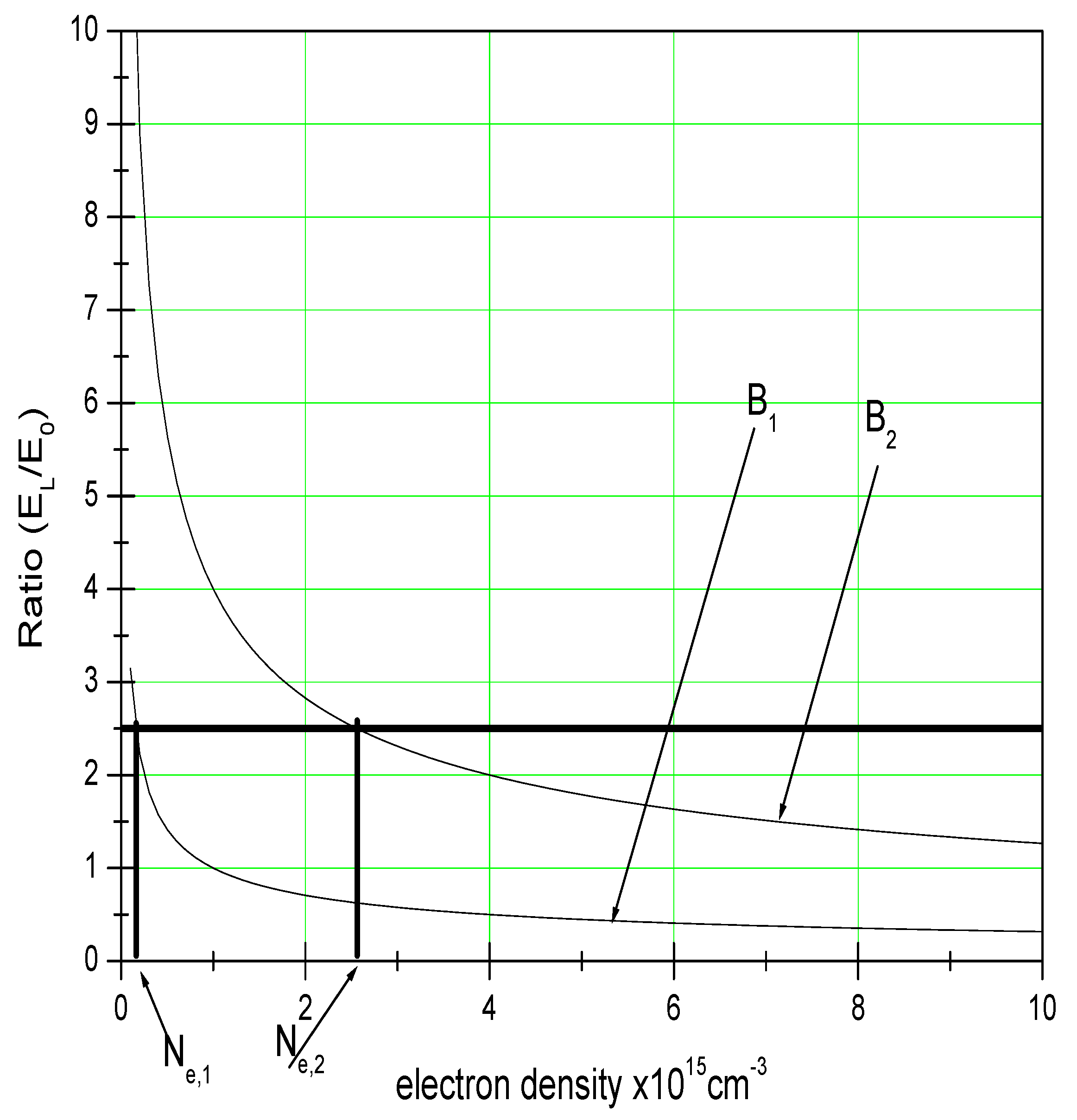
By replacing V by its mean thermal value and assuming equal emitter and plasma particle temperatures, the ratio between the typical Lorentz and electric fields is given by:

$$\frac{E_L}{E_0}=2330·B·\frac{T^{1/2}}{N^{2/3}}.$$

(5)

This ratio is presented in Figure 1 as a function of density for different magnetic field.

For high temperatures, and when the density is low, the effect of the Lorentz field may become important, or even exceed the Stark effect. Thus, under certain conditions, the MSE may compete or even dominate the Stark effect.

3. The Spectral Line

In the presence of an external magnetic field, the total probability (for all directions) of emission of radiation is proportional to the squared modulus ${\left|〈n^{\prime }{l}^{\prime }{m}^{\prime }\left|d_{-m}\right|njm〉\right|}^2$. However, the relative intensity of the Zeeman components when observed in a particular direction (relative to the direction of the magnetic field applied to the source) is of greater interest. The probability of emission (and therefore the line strength), in a given direction $\mathbf{n}$, is proportional to ${\displaystyle \sum }{\left|e^{*}·d_{fi}\right|}^2$ [12], where the summation is over the two independent polarizations, $\mathbf{e}$, which are possible for a given $\mathbf{n}$. For example, if the observation is done along the field (along the z-axis), this sum is given by:

$$|d_x{|}^2+{\left|d_y\right|}^2.$$

(6)

This means that only two $\sigma$ components $(m=\pm 1)$ are observed in the longitudinal direction (along the field).

For observation in the perpendicular direction, the intensity is proportional to the sum:

$$|d_y{|}^2+{\left|d_z\right|}^2.$$

(7)

In the formalism of an emission lines’ profile of an ion emitter immersed in plasma, the intensity of the line is given by the Fourier transform of the autocorrelation function of the dipole:

$$I\left(\omega \right)={\int }_0^{\infty }exp\left(-i\omega t\right)C_{dd}\left(t\right)dt.$$

(8)

The calculation of this function in the case of the longitudinal observation is then given by:

$$I\left(\omega \right)=Re{\int }_0^{\infty }dtexp(-i\omega t)C_{d_x{d}_x}\left(t\right)+Re{\int }_0^{\infty }dtexp(-i\omega t)C_{d_y{d}_y}\left(t\right).$$

(9)

The dipole operator evolution is governed by the evolution operator given by ($\hslash =1$):

$$T_E\left(t\right)=exp[-it\left(H(\overrightarrow{E},\overrightarrow{B})\right)]$$

(10)

where:

$$H(\overrightarrow{E},\overrightarrow{B})=H_0+\frac{q_e}{2m}\overrightarrow{B}\left(\overrightarrow{L}+2\overrightarrow{S}\right)+\overrightarrow{d}\overrightarrow{E}+\overrightarrow{d}\left(\overrightarrow{V}\times \overrightarrow{B}\right)$$

(11)

where the structure fine is not considered. The dipolar part in the Hamiltonian (2):

$$\overrightarrow{d}·\overrightarrow{E}+\overrightarrow{d}·\left(\overrightarrow{V}\times \overrightarrow{B}\right)=q_e\left(E_{x}x+E_{y}y+E_{z}z\right)+\frac{q_{e}B}{c}\left(x{V}_y-y{V}_x\right)$$

(12)

possess only off-diagonal matrix elements whereas the magnetic part (the second term in (11)) is diagonal:

$$\langle n{l}^{\prime }{m}^{\prime }|\frac{q_e}{2m}(L_z+1)|nlm\rangle =\hslash {\omega }_0(m+1){\delta }_{l{l}^{\prime }}{\delta }_{m{m}^{\prime }}$$

(13)

where ${\omega }_0$ is the angular frequency given by the Larmor equation:

$${\omega }_0=-\frac{q_e}{2m}B.$$

(14)

The x-dipolar autocorrelation function has the following expression:

$$C_{d_x{d}_x}\left(t\right)=\sum _{\alpha \beta {\alpha }^{\prime }{\beta }^{\prime }}{d}_{\alpha \beta }^x{\left\{〈\beta \left|T_b^{*}\right|{\beta }^{\prime }〉〈\alpha \left|T_a\right|\alpha 〉\right\}}_{av}{d}_{{\alpha }^{\prime }{\beta }^{\prime }}^{*x}$$

(15)

The averaging subscript ($av$) will be defined later. The evolution operator $T_b^{*}$ acts on the lower level $(n=1)$. Only the magnetic part in $T_b^{*}$ contributes and gives an extra exponential factor $exp(-i{\omega }_{0}t)$ due to the relation (13). Then the last equation becomes:

$$C_{d_x{d}_x}\left(t\right)=exp(-i{\omega }_{0}t)\sum _{\alpha \beta {\alpha }^{\prime }{\beta }^{\prime }}{\delta }_{\beta {\beta }^{\prime }}{d}_{\alpha \beta }^x{\left\{〈\alpha \left|T_a\right|\alpha 〉\right\}}_{av}{d}_{{\alpha }^{\prime }{\beta }^{\prime }}^{*x}$$

(16)

or:

$$C_{d_x{d}_x}\left(t\right)=exp(-i{\omega }_{0}t)\sum _{\alpha \beta {\alpha }^{\prime }{\beta }^{\prime }}{d}_{\alpha ,100}^x{\left\{〈\alpha \left|T_a\right|\alpha 〉\right\}}_{av}{d}_{{\alpha }^{\prime },100}^{*x}$$

(17)

where the vector column:

$$d_{\alpha ,100}^x=\left(\begin{array}{c}<100|d_x|200>=0\\ <100|d_x|21-1>=q\\ <100|d_x|210>=0\\ <100|d_x|211>=-q\end{array}\right).$$

(18)

Note by $|1>=|200>,|2>=|21-1>,|3>=|210>,|4>=|211>$, then $C_{d_x{d}_x}\left(t\right)$ can be easily transformed to:

$$C_{d_x{d}_x}\left(t\right)=q^{2}exp(-i{\omega }_{0}t){\left[\langle 2|T_a|2\rangle +\langle 4|T_a|4\rangle -2Re\langle 2|T_a|4\rangle \right]}_{av}.$$

(19)

As the last term is zero, the x-dipolar autocorrelation function is given by:

$$C_{d_x{d}_x}\left(t\right)=q^2{\left[exp(-i{\omega }_{0}t)\langle 2|{\tilde{T}}_a|2\rangle +exp(+i{\omega }_{0}t)\langle 4|{\tilde{T}}_a|4\rangle \right]}_{av}.$$

(20)

The same technique used in [13], applies to compute $\langle 2\left|{\tilde{T}}_a\right|2\rangle$ and $\langle 4\left|{\tilde{T}}_a\right|4\rangle$, and the x-dipolar autocorrelation function becomes (after inserting the collision operator ${\mathsf{\Phi }}_e$ which takes into account the magnetic field [1]):

$$\begin{array}{c}\hfill C_{d_x{d}_x}\left(t\right)=q^{2}exp(-{\mathsf{\Phi }}_{e}t)(exp(-i{\omega }_{0}t)+exp(+i{\omega }_{0}t))[2+cos\left(\eta h\left(t\right)\right)]=\\ \hfill 2exp(-{\mathsf{\Phi }}_{e}t)cos\left({\omega }_{0}t\right)[2+cos\left(\eta h\left(t\right)\right)]\end{array}$$

(21)

where $\eta =D/\hslash$ and:

$$h\left(t\right)=\sqrt{2{\int }_0^{t}d\tau (t-\tau )<\overrightarrow{E\left(\tau \right)}\overrightarrow{E\left(0\right)}>}$$

(22)

and

$$\overrightarrow{E\left(t\right)}={\overrightarrow{E}}_{Stark}\left(t\right)+{\overrightarrow{E}}_{Lorentz}\left(t\right).$$

(23)

Neglecting the correlation between the Stark and Lorentz microfield, we can write:

$$<\overrightarrow{E\left(\tau \right)}\overrightarrow{E\left(0\right)}>=C_{Stark}^{EE}\left(t\right)+C_{Lorentz}^{EE}\left(t\right)$$

(24)

where:

$$C_{Stark}^{EE}\left(t\right)=<{\overrightarrow{E}}_{Stark}\left(t\right){\overrightarrow{E}}_{Stark}\left(0\right)>$$

(25)

is the Stark microfield auto-correlation function and

$$C_{Lorentz}^{EE}\left(t\right)=<{\overrightarrow{E}}_{Lorentz}\left(t\right){\overrightarrow{E}}_{Lorentz}\left(0\right)>=B^2<\overrightarrow{V}\left(t\right)\overrightarrow{V}\left(0\right)>=B^2{C}_{VV}\left(t\right)$$

(26)

is the Lorentz microfield auto-correlation function. The first correlation function $C_{Stark}^{EE}\left(t\right)$ is given by [11] valid for neutral emitters:

$$C_{Stark}^{EE}\left(t\right)=\frac{3r_0}{{\lambda }_D\sqrt{\pi }}\frac{1}{t}[1+t^2-t\sqrt{\pi }(t^2+3/2)exp\left(t^2\right)erfc\left(t\right)]$$

(27)

where t is the time expressed in units of the plasma frequency, and ${\lambda }_D$ the electronic Debye length and $r_0$ is the mean distance between atoms.

The second correlation function $C_{Doppler}^{EE}\left(t\right)$ is given in the Brownian model by Hansen [14] valid for neutral emitters:

$$C_{Lorentz}^{EE}\left(t\right)=B^2\frac{kT}{m}exp(-\frac{3kT}{2m{D}_v}t)$$

(28)

where $D_v$ is the self diffusion coefficient and k is the Boltzmann constant. In the case of the static approximation, the x-dipolar autocorrelation function reads:

$$C_{d_x{d}_x}\left(t\right)=2exp(-{\mathsf{\Phi }}_{e}t)cos\left({\omega }_{0}t\right)[2+cos\left(\eta t\sqrt{<E^2>+B^2<V^2>}\right)].$$

(29)

The contribution of the y-component (second term in (9)) is the same as the x-component in the expression of intensity:

$$I\left(\omega \right)=2Re{\int }_0^{\infty }dtexp(-i\omega t)C_{d_x{d}_x}\left(t\right).$$

(30)

4. Results and Discussion

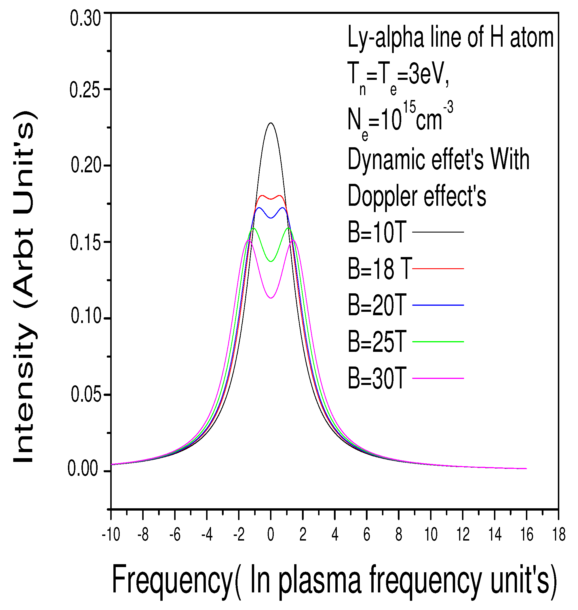
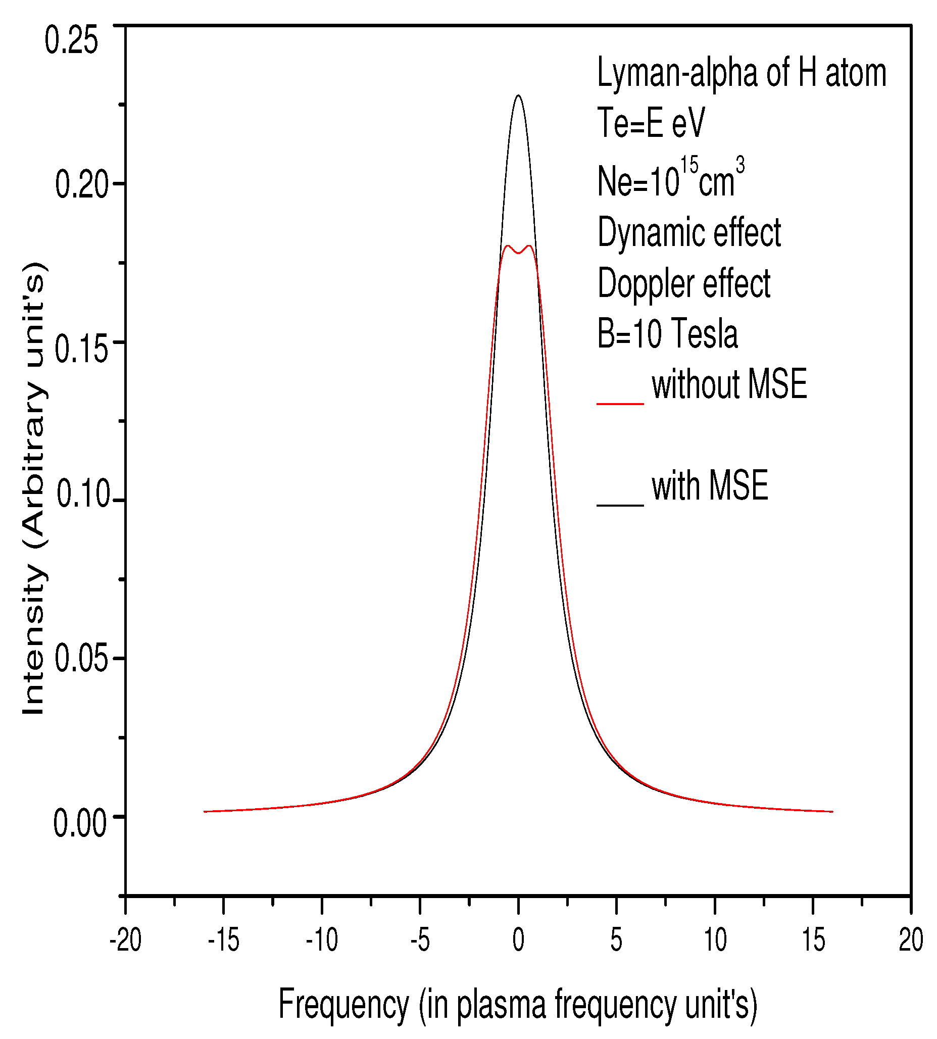
We first performed a set of calculations (Figure 2, Figure 3, Figure 4, Figure 5 and Figure 6), taking account of the MSE to determine the parameters for which a spectroscopically important MSE could appear. Clearly, the Zeeman splitting made sure of a measurable B-field and this must survive the Stark and Doppler broadening, if the B field is to be measured. Figure 2 shows the estimate range of parameters for which the Zeeman splitting remains visible. In Figure 3, we refine this estimate by also taking the Doppler broadening into account. All calculations compute the Lyman-alpha line in Hydrogen plasmas for a strong B-field for a parallel direction of observation, at several conditions of temperature and densities.

All spectral lines are in arbitrary units and frequencies are in the plasma frequency unit. Figure 2 and Figure 3 are for an electron density $Ne={10}^{15}$ cm${}^{-3}$ and temperature $T=3$ eV. The MSE is taken into account. Figure 2 is without the Doppler effect and Figure 3 is with the Doppler effect. Figure 2 is for different magnetic fields in the range [1 Tesla–10 Tesla], whereas Figure 3 is for the range [10 Tesla, 30 Tesla]. We also note from these two figures that the Doppler effect and MSE are in competition in the formation of the line profile: When the Doppler effect is absent, the MSE is immediately manifested as soon as B exceeds 1 Tesla, and when the Doppler effect is present, the MSE begins to manifest from $B=18$ Tesla. Figure 4 further confirms this: If the magnetic field B is not strong enough ($B<18$ Tesla), the Doppler effect and MSE are increasingly accentuated with the temperature so that they hide the Zeeman effect.

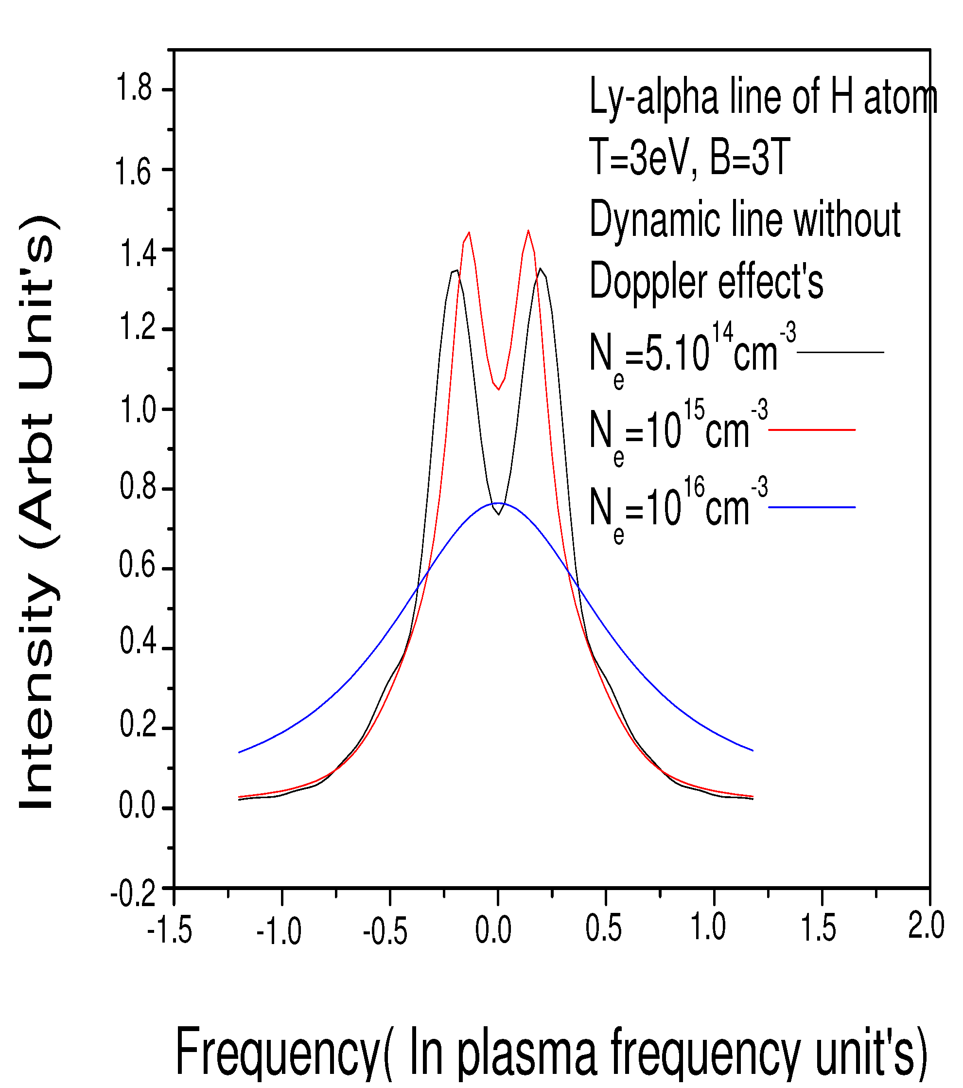
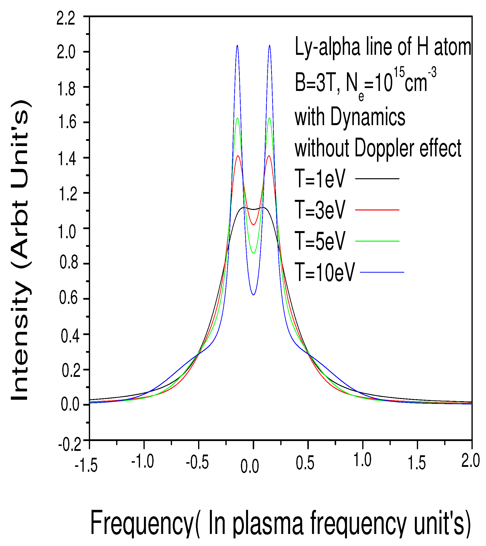
Figure 5 shows the effect of the density on the spectral line when the Doppler effect is not considered: The Zeeman effect was found to be quite pronounced for densities that are less than $Ne={10}^{16}$ cm${}^{-3}$. For higher densities, the fine structure must be taken into account. Figure 6 shows the effect of the temperature on the spectral line when the Doppler effect is not considered: The Zeeman effect was found to become increasingly pronounced as the temperature decreases. For temperatures above 10 eV, the fine structure must also be taken into account.

5. Conclusions

In this work we have presented new results concerning the broadening of the hydrogen spectral line at the edge of a Tokamak, where Doppler broadening is dominant over fine structure, electronic broadening, ion Stark broadening, the MSE, and Zeeman separation.The study showed that when the magnetic field is larger than 10 Tesla, Zeeman separation becomes visible. For less intense magnetic fields, the Doppler effect is discarded, the Zeeman effect for different values of the magnetic field could be seen. The relative importance of the MSE compared to Stark broadening was more pronounced for high temperatures and low densities.

References

- Touati, K. Analyse Spectroscopique des Plasmas en présence d’un Champ Magnétique. Ph.D. Thesis, Université of Provence, Marseille, France, 2003. [Google Scholar]
- Rosato, J.; Marandet, Y.; Peiffer, A.; Capes, H.; Godbert-Mouret, L.; Koubiti, M.; Stamm, R. Modeling of Stark-broadened lines in a fluctuating edge plasma. Contrib. Plasma Phys. 2014, 54, 565. [Google Scholar] [CrossRef]
- Touati, K.; Meftah, M.T. Line Shapes in the Magnetized Plasmas. J. Mod. Phys. 2012, 3, 943–946. [Google Scholar] [CrossRef] [Green Version]
- Rosato, J.; Capes, H.; Godbert-Mouret, L.; Koubiti, M.; Marandet, Y.; Rosmej, F.; Stamm, R. Modeling of Stark Profiles in a Fluctuating Edge Tokamak Plasma. Contrib. Plasma. Phys. 2006. [Google Scholar] [CrossRef]
- Hoe, N.; Drawin, H.W.; Herman, L. Effect of a Uniform Magnetic Field on the Line Profiles of the Hydrogen. J. Quant. Spectrosc. Transf. Radiat. 1967, 7, 429. [Google Scholar] [CrossRef]
- Griem, H.R.; Kolb, A.; Chen, Y. Stark broadening of neutral helium lines in a plasma. Phys. Rev. 1959, 116, 4. [Google Scholar] [CrossRef]
- Griem, H.R.; et Blaha, M.; Keepple, P.C. Stark-profile calculations for Lyman-series lines of one-electron ions in dense plasmas. Phys. Rev. A 1979, 19, 2421. [Google Scholar] [CrossRef]
- Alexiou, S. Erratum: Z scaling of the 3P-3S Li isoelectronic series transition: Quadrupole Stark broadening and resonances. Phys. Rev. A 1994, 49, 106. [Google Scholar] [CrossRef] [PubMed]
- Alexiou, S. Line Shapes in a Magnetic Field: Trajectory Modifications I: Electrons. Atoms 2019, 7, 52. [Google Scholar] [CrossRef] [Green Version]
- Alexiou, S. Line Shapes in a Magnetic Field: Trajectory Modifictions II: Full Collision-Time Statistics. Atoms 2019, 7, 94. [Google Scholar] [CrossRef] [Green Version]
- Brissaud, A.; Goldbach, C.; Léorat, J.; Mazure, A.; Nollez, G. On the validity of the model microfield method as applied to Stark broadening of neutral lines. J. Phys. B 1976, 9. [Google Scholar] [CrossRef]
- Berestetskii, V.B.; Lifchitz, E.M.; Pitaevskii, L.P. Course of Theoretical Physics, 2nd ed.; Pergamon Press: Oxford, UK, 1982; Volume 4, Chapter V, Section 51. [Google Scholar]
- Bouguettaia, H.; Chihi, I.; Chenini, K.; Meftah, M.T.; Khelfaoui, F.; Stamm, R. Application of path integral formalism in spectral line broadening: Lyman-α in hydrogenic plasma. JQSRT 2005, 94, 335–346. [Google Scholar] [CrossRef]
- Hansen, J.P.; McDonald, I.R. Theory of Simple Liquids, 3rd ed.; Academic Press: Cambridge, MA, USA, 2005. [Google Scholar]
Figure 1.
The ratio of the Lorentz to the Stark field for two different magnetic fields.
Figure 2.
Lyman Alpha line in the hydrogen plasma with the Motional Stark Effect (MSE) and without the Doppler and fine structure effects.
Figure 3.
Lyman Alpha line in the hydrogen plasma with the MSE and Doppler effects and without the fine structure effect.
Figure 4.
Lyman Alpha line in the hydrogen plasma: A comparison between with and without the MSE. With the Doppler effects and without the fine structure effect. The same plasma conditions are the same as Figure 3.
Figure 5.
Lyman Alpha line in the hydrogen plasma: The electron density effect with the MSE effect and without Doppler and fine structure effects.
Figure 6.
Lyman Alpha line in the hydrogen plasma: The electron temperature effect on the line with the MSE effect without the Doppler effect and fine structure effects.
Publisher’s Note: MDPI stays neutral with regard to jurisdictional claims in published maps and institutional affiliations. |
© 2020 by the authors. Licensee MDPI, Basel, Switzerland. This article is an open access article distributed under the terms and conditions of the Creative Commons Attribution (CC BY) license (http://creativecommons.org/licenses/by/4.0/).
Share and Cite
MDPI and ACS Style
Touati, K.A.; Chenini, K.; Meftah, M.T. Stark-Zeeman Broadening of Spectral Line Shapes in Magnetized Plasmas. Atoms 2020, 8, 91. https://0-doi-org.brum.beds.ac.uk/10.3390/atoms8040091
AMA Style
Touati KA, Chenini K, Meftah MT. Stark-Zeeman Broadening of Spectral Line Shapes in Magnetized Plasmas. Atoms. 2020; 8(4):91. https://0-doi-org.brum.beds.ac.uk/10.3390/atoms8040091
Chicago/Turabian StyleTouati, Kamel Ahmed, Keltoum Chenini, and Mohammed Tayeb Meftah. 2020. "Stark-Zeeman Broadening of Spectral Line Shapes in Magnetized Plasmas" Atoms 8, no. 4: 91. https://0-doi-org.brum.beds.ac.uk/10.3390/atoms8040091
Note that from the first issue of 2016, this journal uses article numbers instead of page numbers. See further details here.