Broad UV Emission Lines in Type-1 Active Galactic Nuclei: A Note on Spectral Diagnostics and the Excitation Mechanism

 ,
,  ,
,  and
and
Abstract
:1. Introduction
Quasar Spectra: Emission from Mildly Ionized Gas
2. The UV Emission Lines
- The Ly + Nv1240 blend: The of the Nv1240 parent ionic species ≈ 78 eV is the highest among the line considered here. The Nv1240 is due to a resonant transition () in the lithium isoelectronic configuration;
- The 1400 Å blend [26]: The Siiv doublet is also a resonant doublet (, from the sodium isoelectronic configuration, ). The creation ionization potential of Si is much lower, ≈34 eV, than the one of N. The Oiv]1402 inter-combination multiplet is due to transitions between a term and term where the first term is at 0.04785 eV above ground level, with critical densities in the range – cm−3 [27,28];
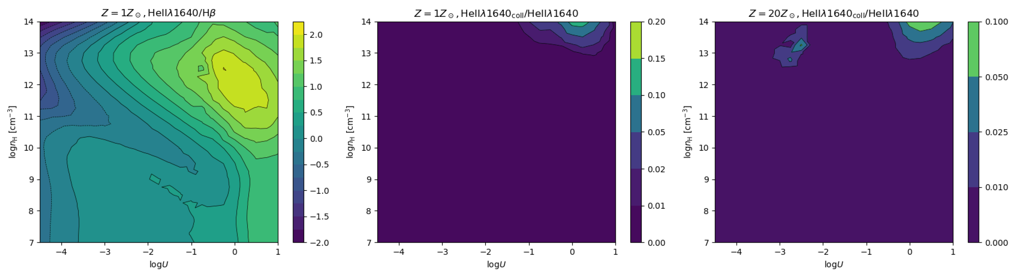
- The Civ+ Heii1640 blend: The Civ line is a resonant doublet () and is again emitted by a transition in the lithium isoelectronic configuration. The parent ionic species has an ionization potential of ≈50 eV. Heii1640 is emitted via 3d 2D → 2p 2P, which corresponds to a transition between two very high energy levels above the ground state (48 and 40 eV). The Heii1640 line is blended with the red side of Civ, and the two lines are often measured together [29].
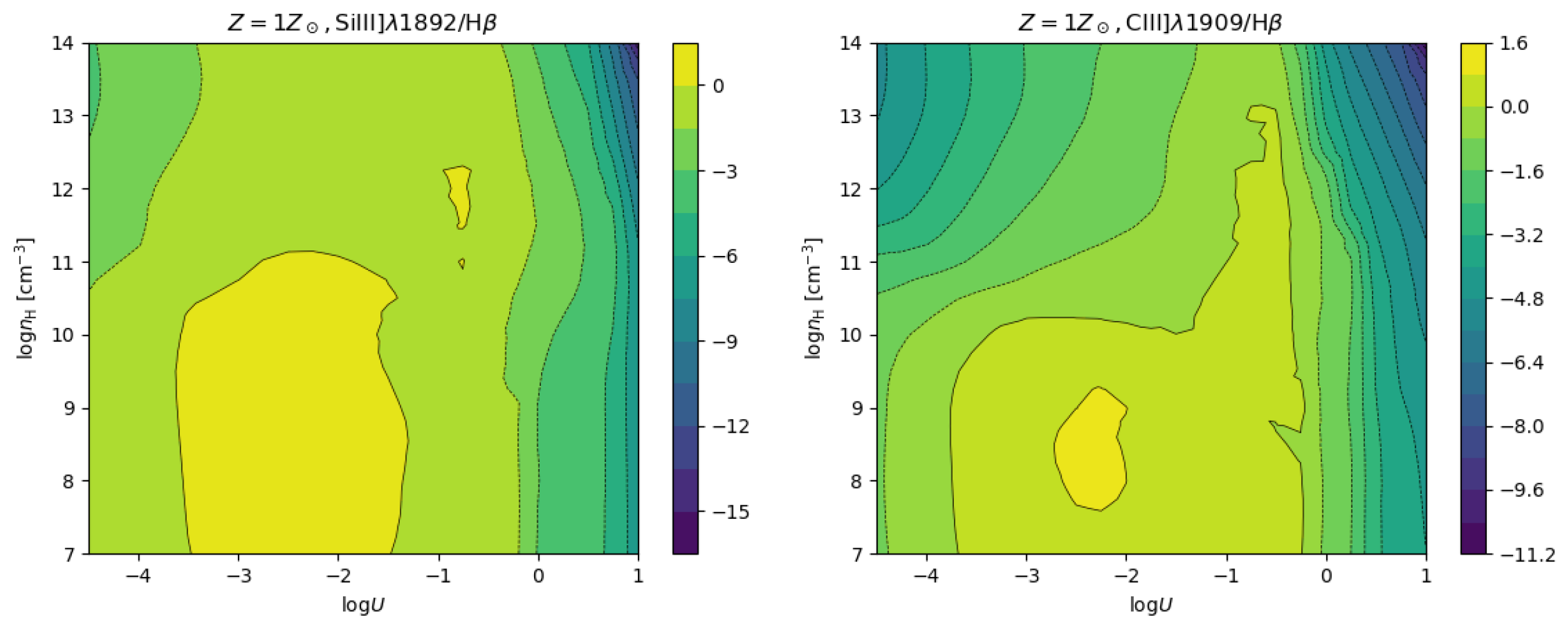
- The blend at Å is due, in most part, to the Aliii1860 doublet and to the Siiii]1892 and Ciii]1909 lines. Aliii is a resonant doublet as Civ () in the sodium isoelectronic configuration, while Siiii] and Ciii] are due to inter-combination transitions () with widely different critical densities (≈ cm−3 and ≈ cm−3, respectively; [18]). The parent ionic species imply ionization potentials eV, intermediate between the ones of the LILs and of the HILs; 40–50 eV.
3. Photoionization Computations
- the ionization parameter , where is the number of ionizing photons and the distance between the continuum source and the line emitting gas, provides the ratio between the hydrogen-ionizing photon and the hydrogen number density;
- the hydrogen density ;
- the metallicity Z;
- the quasar spectral energy distribution (SED);
- the column density ;
- a micro-turbulence parameter [8].
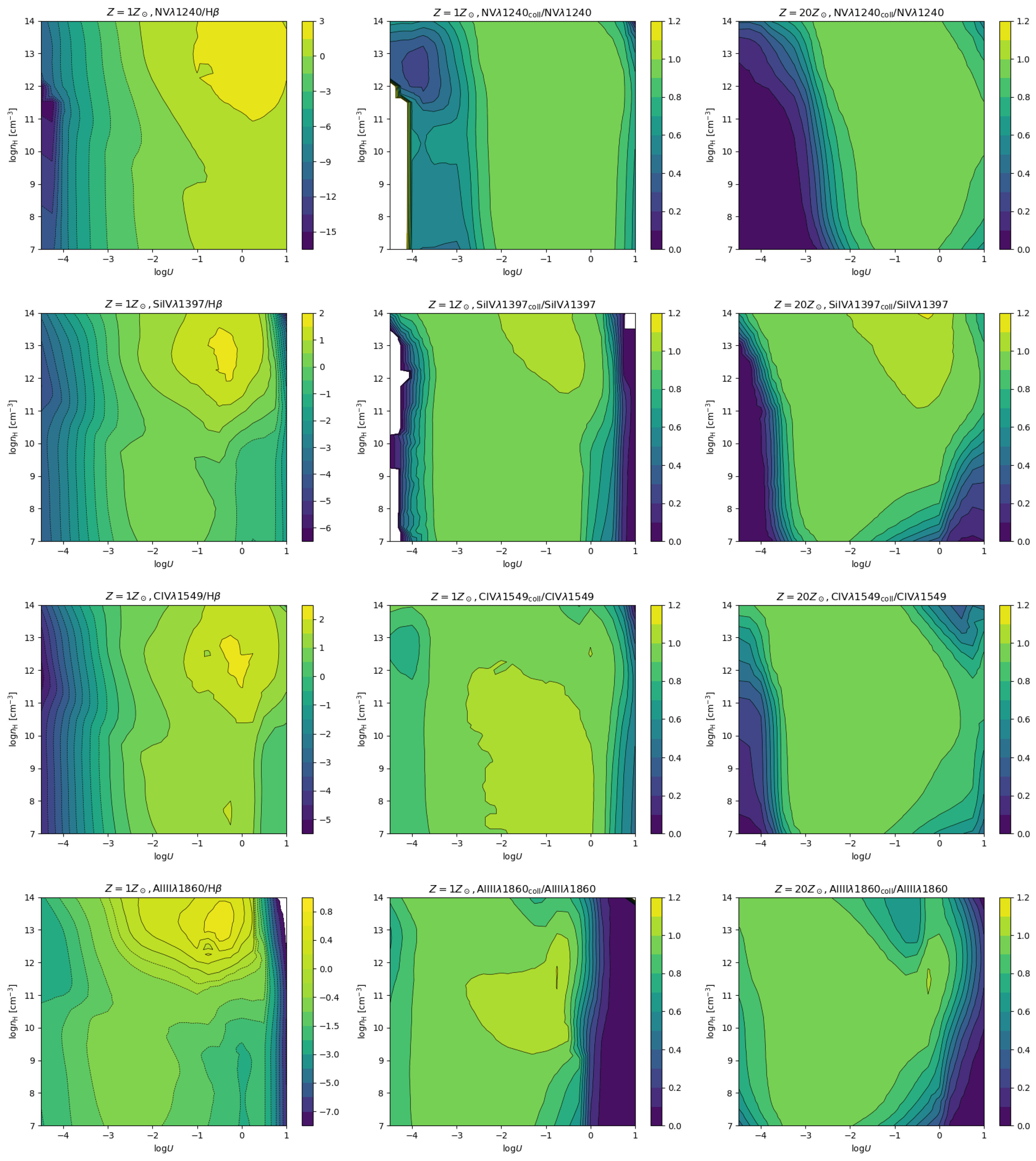
4. Results
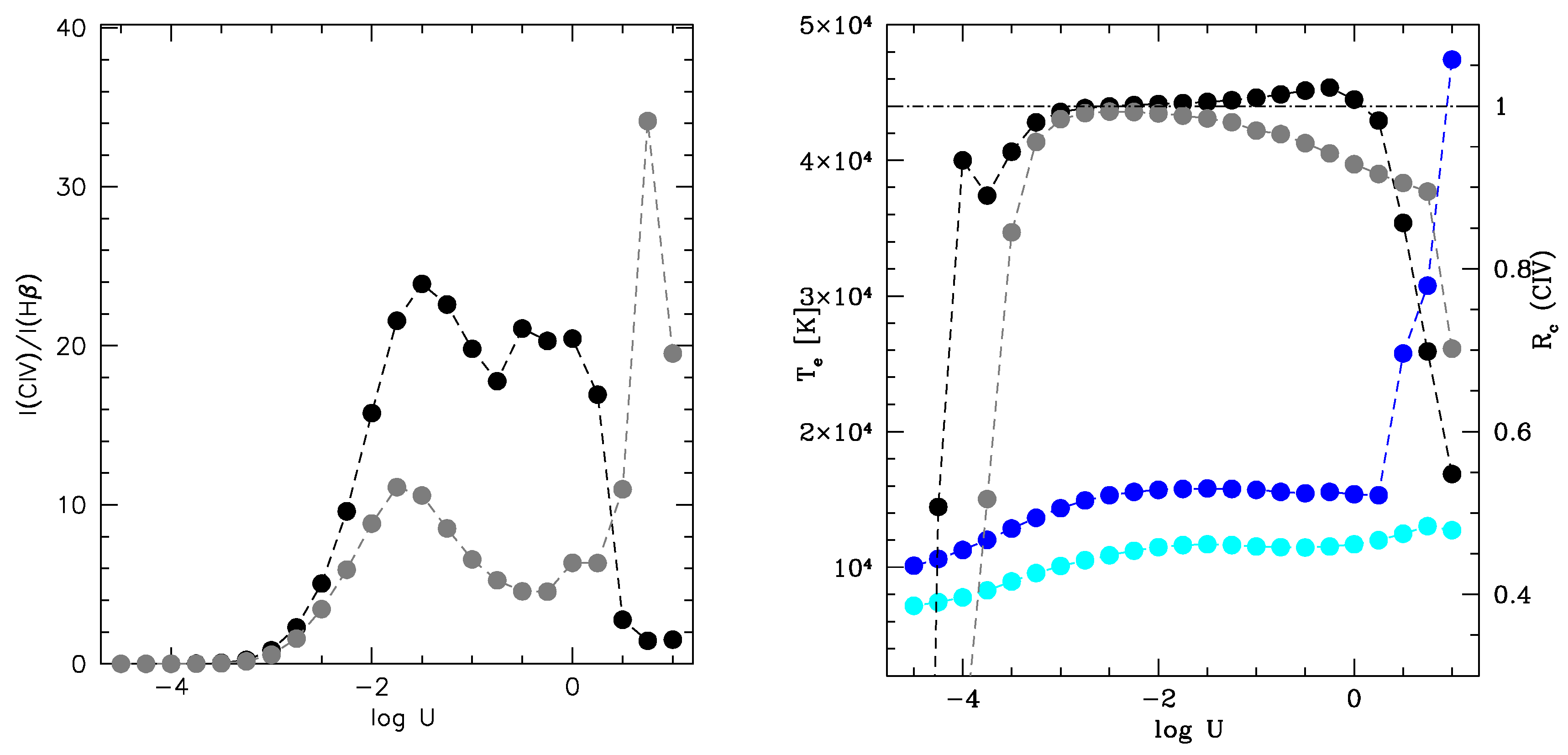
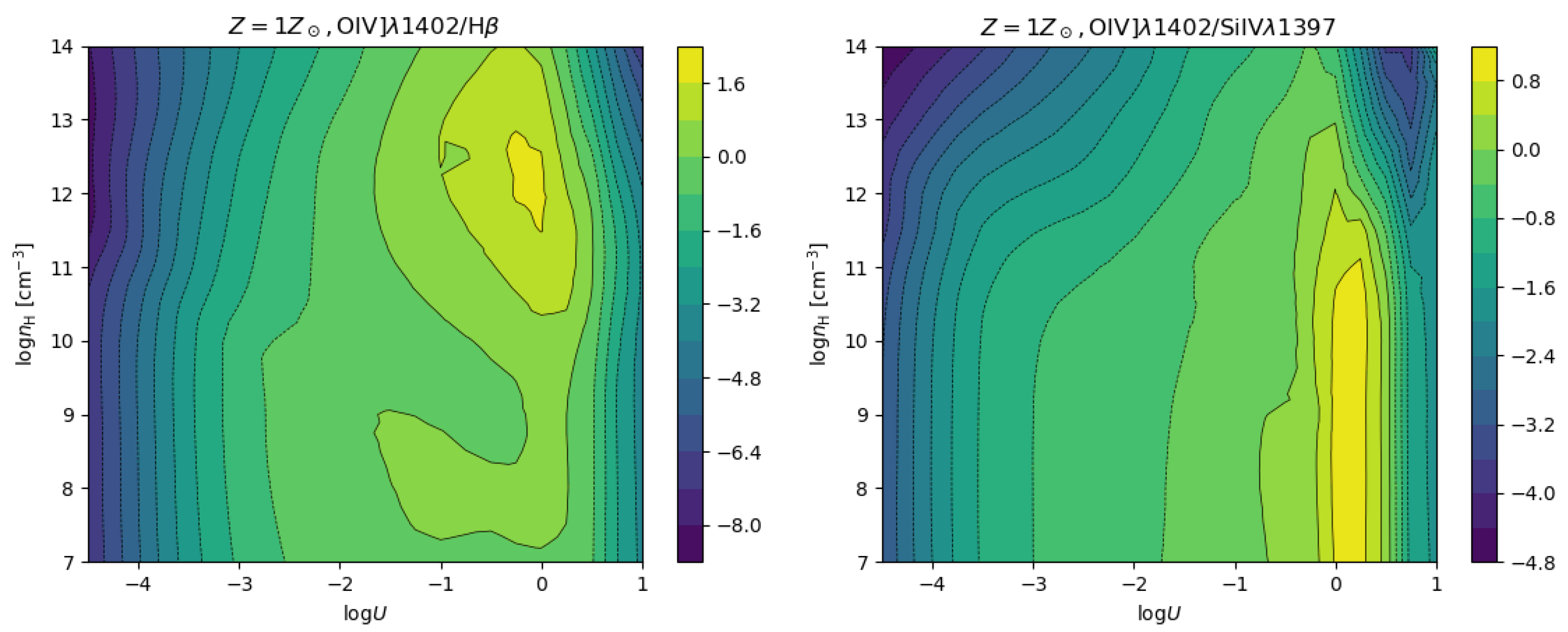
4.1. Trends with the Ionization Parameter and Density
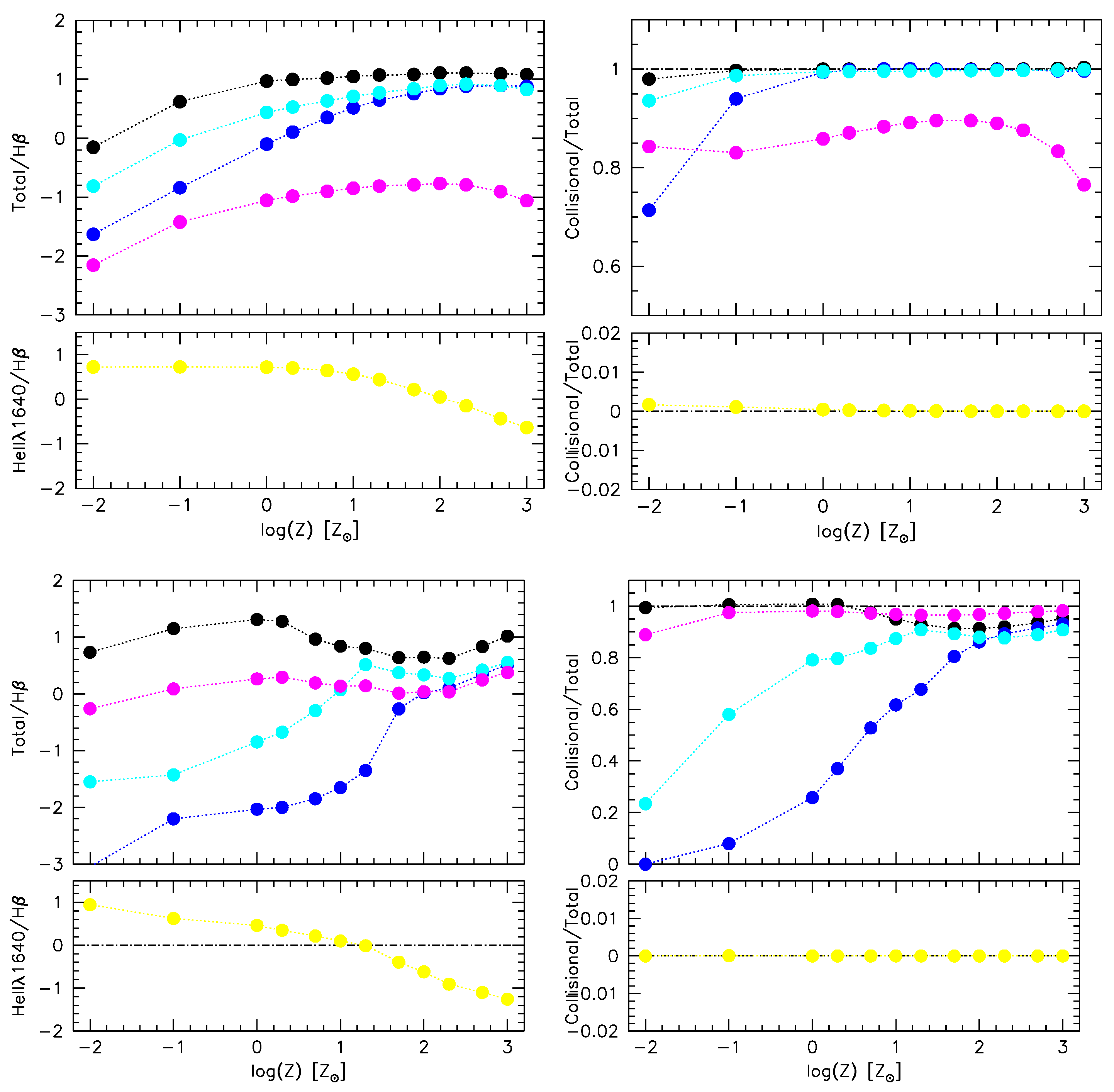
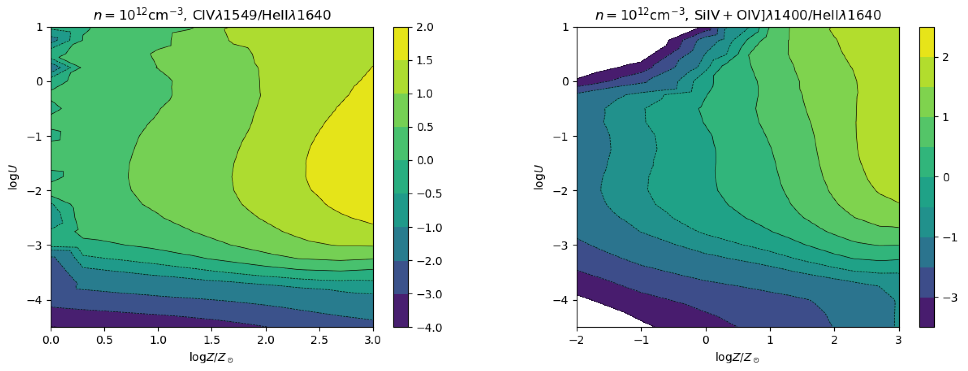
4.2. Dependence on Metallicity
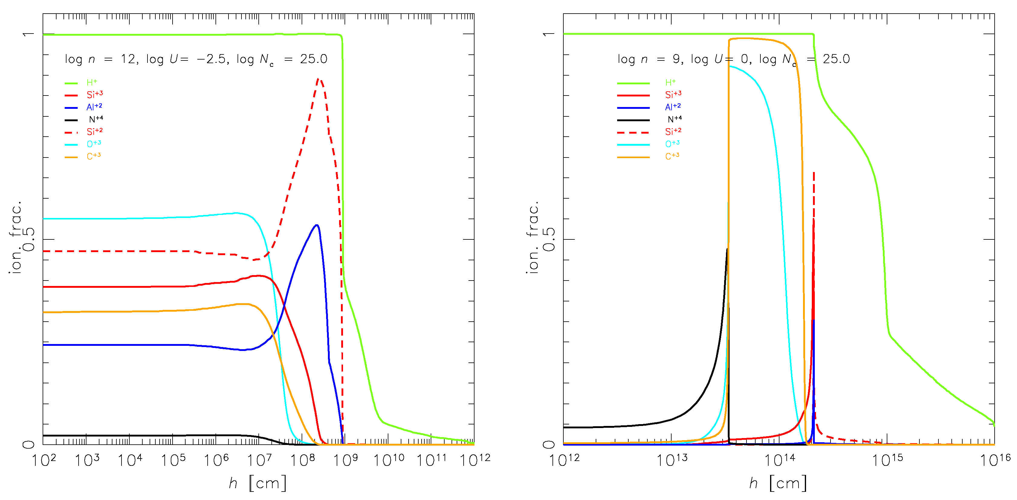
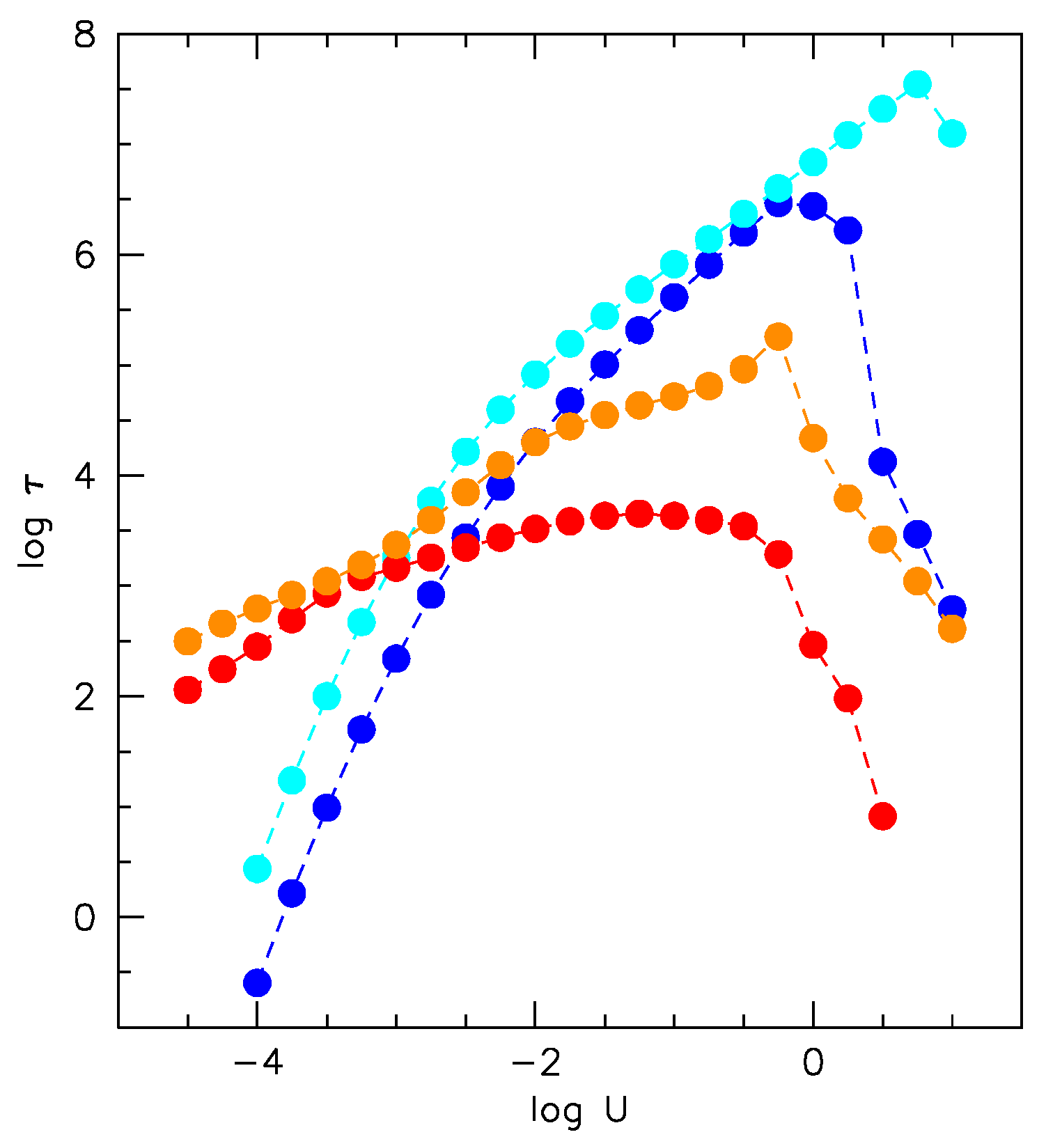
4.3. Dependence on Column Density and on Optical Depth
5. Discussion
5.1. BLR Physical Conditions along the Quasar Main Sequence
5.2. BLR Radius
5.3. Diagnostic Ratios to Estimate Metallicity Content within the BLR
5.4. Feedback Effects of Accreting Black Holes
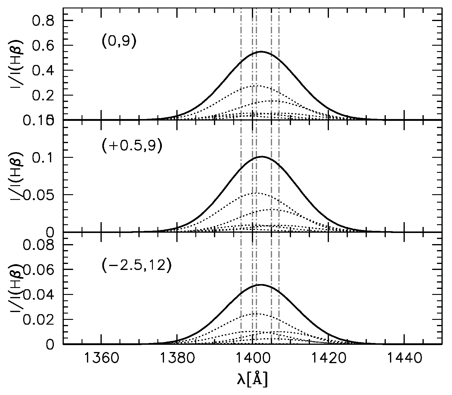
5.5. Applications to Empirical Line Profile Modeling: Intensity Ratios of the Doublet Components
5.6. Applications to Empirical Line Profile Modeling: The Case of Oiv]1402
6. Summary and Conclusions
Author Contributions
Funding
Acknowledgments
Conflicts of Interest
Abbreviations
| AGN | active galactic nucleus |
| BLR | broad line region |
| EC | Electronic configuration |
| FIZ | fully ionized zone |
| FWHM | full-width half-maximum |
| HIL | high-ionization line |
| IIL | intermediate-ionization line |
| LIL | low-ionization line |
| MS | main sequence |
| NLSy1 | Narrow-Line Seyfert 1 |
| PIZ | partially ionized zone |
Appendix A. Electron-Ion Collisions
References
- Netzer, H. AGN emission lines. In Active Galactic Nuclei; Blandford, R.D., Netzer, H., Woltjer, L., Courvoisier, T.J.-L., Mayor, M., Eds.; Springer: Berlin, Germany, 1990; pp. 57–160. [Google Scholar]
- Peterson, B.M. An Introduction to Active Galactic Nuclei; Cambridge University Press: Cambridge, UK, 1997. [Google Scholar]
- Osterbrock, D.E.; Ferland, G.J. Astrophysics of Gaseous Nebulae and Active Galactic Nuclei; University Science Books: Mill Valley, CA, USA, 2006. [Google Scholar]
- Boroson, T.A.; Green, R.F. The emission-line properties of low-redshift quasi-stellar objects. Astrophys. J. Suppl. Ser. 1992, 80, 109–135. [Google Scholar] [CrossRef]
- Sulentic, J.W.; Marziani, P.; Dultzin-Hacyan, D. Phenomenology of Broad Emission Lines in Active Galactic Nuclei. Annu. Rev. Astron. Astrophys. 2000, 38, 521–571. [Google Scholar] [CrossRef]
- Shen, Y.; Ho, L.C. The diversity of quasars unified by accretion and orientation. Nature 2014, 513, 210–213. [Google Scholar] [CrossRef] [PubMed] [Green Version]
- Marziani, P.; Sulentic, J.W.; Negrete, C.A.; Dultzin, D.; Zamfir, S.; Bachev, R. Broad-line region physical conditions along the quasar eigenvector 1 sequence. Mon. Not. R. Astron. Soc. 2010, 409, 1033–1048. [Google Scholar] [CrossRef] [Green Version]
- Panda, S.; Czerny, B.; Adhikari, T.P.; Hryniewicz, K.; Wildy, C.; Kuraszkiewicz, J.; Śniegowska, M. Modeling of the Quasar Main Sequence in the Optical Plane. Astrophys. J. 2018, 866, 115. [Google Scholar] [CrossRef]
- Panda, S.; Marziani, P.; Czerny, B. The Quasar Main Sequence explained by the combination of Eddington ratio, metallicity and orientation. arXiv 2019, arXiv:1905.01729. [Google Scholar]
- Fraix-Burnet, D.; Marziani, P.; D’Onofrio, M.; Dultzin, D. The Phylogeny of Quasars and the Ontogeny of Their Central Black Holes. Front. Astron. Space Sci. 2017, 4, 1. [Google Scholar] [CrossRef] [Green Version]
- Sulentic, J.W.; Marziani, P.; Zwitter, T.; Dultzin-Hacyan, D.; Calvani, M. The Demise of the Classical Broad-Line Region in the Luminous Quasar PG 1416-129. Astrophys. J. Lett. 2000, 545, L15–L18. [Google Scholar] [CrossRef]
- Sulentic, J.W.; Bachev, R.; Marziani, P.; Negrete, C.A.; Dultzin, D. C IV λ1549 as an Eigenvector 1 Parameter for Active Galactic Nuclei. Astrophys. J. 2007, 666, 757–777. [Google Scholar] [CrossRef] [Green Version]
- Richards, G.T.; Kruczek, N.E.; Gallagher, S.C.; Hall, P.B.; Hewett, P.C.; Leighly, K.M.; Deo, R.P.; Kratzer, R.M.; Shen, Y. Unification of Luminous Type 1 Quasars through C IV Emission. Astrophys. J. 2011, 141, 167. [Google Scholar] [CrossRef]
- Coatman, L.; Hewett, P.C.; Banerji, M.; Richards, G.T. C iv emission-line properties and systematic trends in quasar black hole mass estimates. Mon. Not. R. Astron. Soc. 2016, 461, 647–665. [Google Scholar] [CrossRef] [Green Version]
- Sulentic, J.W.; del Olmo, A.; Marziani, P.; Martínez-Carballo, M.A.; D’Onofrio, M.; Dultzin, D.; Perea, J.; Martínez-Aldama, M.L.; Negrete, C.A.; Stirpe, G.M.; et al. What does Civλ1549 tell us about the physical driver of the Eigenvector Quasar Sequence? Astron. Astrophys. 2017, 608, A122. [Google Scholar] [CrossRef] [Green Version]
- Vietri, G.; Piconcelli, E.; Bischetti, M.; Duras, F.; Martocchia, S.; Bongiorno, A.; Marconi, A.; Zappacosta, L.; Bisogni, S.; Bruni, G.; et al. The WISSH Quasars Project IV. BLR versus kpc-scale winds. arXiv 2018, arXiv:1802.03423. [Google Scholar]
- Leighly, K.M. Hubble Space Telescope STIS Ultraviolet Spectral Evidence of Outflow in Extreme Narrow-Line Seyfert 1 Galaxies. II. Modeling and Interpretation. Astrophys. J. 2004, 611, 125–152. [Google Scholar] [CrossRef]
- Negrete, A.; Dultzin, D.; Marziani, P.; Sulentic, J. BLR Physical Conditions in Extreme Population A Quasars: A Method to Estimate Central Black Hole Mass at High Redshift. Astrophys. J. 2012, 757, 62. [Google Scholar] [CrossRef]
- Marinello, A.O.M.; Rodriguez-Ardila, A.; Garcia-Rissmann, A.; Sigut, T.A.A.; Pradhan, A.K. The FeII emission in active galactic nuclei: Excitation mechanisms and location of the emitting region. Astrophys. J. 2016, 820, 116. [Google Scholar] [CrossRef] [Green Version]
- Peterson, B.M.; Ferrarese, L.; Gilbert, K.M.; Kaspi, S.; Malkan, M.A.; Maoz, D.; Merritt, D.; Netzer, H.; Onken, C.A.; Pogge, R.W.; et al. Central Masses and Broad-Line Region Sizes of Active Galactic Nuclei. II. A Homogeneous Analysis of a Large Reverberation-Mapping Database. Astrophys. J. 2004, 613, 682–699. [Google Scholar] [CrossRef] [Green Version]
- Peterson, B.M. Space Telescope and Optical Reverberation Mapping Project: A Leap Forward in Reverberation Mapping. IAU Symp. 2017, 324, 215–218. [Google Scholar] [CrossRef] [Green Version]
- Collin-Souffrin, S.; Dumont, A.M. Emission spectra of weakly photoionized media in active nuclei of galaxies. Astron. Astrophys. 1989, 213, 29–48. [Google Scholar]
- Collin, S.; Joly, M. The Fe II problem in NLS1s. New Astron. Rev. 2000, 44, 531–537. [Google Scholar] [CrossRef] [Green Version]
- Panda, S.; Czerny, B.; Wildy, C.; Śniegowska, M. What Drives the Quasar Main Sequence? Bajan, K., Biernacka, M., Pollo, A., Eds.; Introduction to Cosmology, 3rd Cosmology School: Cracow, Poland, 2019; Volume 9, pp. 199–202. [Google Scholar]
- Negrete, C.A.; Dultzin, D.; Marziani, P.; Sulentic, J.W. A New Method to Obtain the Broad Line Region Size of High Redshift Quasars. Astrophys. J. 2014, 794, 95. [Google Scholar] [CrossRef] [Green Version]
- Wills, D.; Netzer, H. The 1400 A emission feature in quasi-stellar objects. Astrophys. J. 1979, 233, 1–4. [Google Scholar] [CrossRef]
- Zheng, W. The Critical Densities for Some Emission Lines. Astrophys. Lett. Commun. 1988, 27, 275. [Google Scholar]
- Feldman, U. Transitions from Metastable Levels Emitted during Short-Duration Bursts: How Valid Are Their Calculated Intensities? Astrophys. J. 1992, 385, 758. [Google Scholar] [CrossRef]
- Fine, S.; Croom, S.M.; Bland-Hawthorn, J.; Pimbblet, K.A.; Ross, N.P.; Schneider, D.P.; Shanks, T. The CIV linewidth distribution for quasars and its implications for broad-line region dynamics and virial mass estimation. Mon. Not. R. Astron. Soc. 2010, 409, 591–610. [Google Scholar] [CrossRef] [Green Version]
- Mathews, W.G.; Ferland, G.J. What heats the hot phase in active nuclei? Astrophys. J. 1987, 323, 456–467. [Google Scholar] [CrossRef]
- Ferland, G.J.; Done, C.; Jin, C.; Landt, H.; Ward, M.J. State-of-the-art AGN SEDs for photoionization models: BLR predictions confront the observations. Mon. Not. R. Astron. Soc. 2020, 494, 5917–5922. [Google Scholar] [CrossRef]
- Ferland, G.J.; Porter, R.L.; van Hoof, P.A.M.; Williams, R.J.R.; Abel, N.P.; Lykins, M.L.; Shaw, G.; Henney, W.J.; Stancil, P.C. The 2013 Release of Cloudy. Rev. Mex. Astron. Astrofís. 2013, 49, 137–163. [Google Scholar]
- Ferland, G.J.; Chatzikos, M.; Guzmán, F.; Lykins, M.L.; van Hoof, P.A.M.; Williams, R.J.R.; Abel, N.P.; Badnell, N.R.; Keenan, F.P.; Porter, R.L.; et al. The 2017 Release Cloudy. Rev. Mex. Astron. Astrofís. 2017, 53, 385–438. [Google Scholar]
- Shin, J.; Woo, J.H.; Nagao, T.; Kim, S.C. The Chemical Properties of Low-redshift QSOs. Astrophys. J. 2013, 763, 58. [Google Scholar] [CrossRef] [Green Version]
- Nagao, T.; Maiolino, R.; Marconi, A. Gas metallicity in the narrow-line regions of high-redshift active galactic nuclei. Astron. Astrophys. 2006, 447, 863–876. [Google Scholar] [CrossRef] [Green Version]
- Śniegowska, M.; Marziani, P.; Czerny, B.; Panda, S.; Martínez-Aldama, M.L.; del Olmo, A.; D’Onofrio, M. High metal content of highly accreting quasars. arXiv 2020, arXiv:2009.14177. [Google Scholar]
- Nagao, T.; Marconi, A.; Maiolino, R. The evolution of the broad-line region among SDSS quasars. Astron. Astrophys. 2006, 447, 157–172. [Google Scholar] [CrossRef] [Green Version]
- Juarez, Y.; Maiolino, R.; Mujica, R.; Pedani, M.; Marinoni, S.; Nagao, T.; Marconi, A.; Oliva, E. The metallicity of the most distant quasars. Astron. Astrophys. 2009, 494, L25–L28. [Google Scholar] [CrossRef]
- Sulentic, J.W.; Marziani, P.; del Olmo, A.; Dultzin, D.; Perea, J.; Alenka Negrete, C. GTC spectra of z ≈ 2.3 quasars: Comparison with local luminosity analogs. Astron. Astrophys. 2014, 570, A96. [Google Scholar] [CrossRef] [Green Version]
- Negrete, C.A.; Dultzin, D.; Marziani, P.; Sulentic, J.W. Reverberation and Photoionization Estimates of the Broad-line Region Radius in Low-z Quasars. Astrophys. J. 2013, 771, 31. [Google Scholar] [CrossRef] [Green Version]
- Martinez-Aldama, M.L.; Del Olmo, A.; Marziani, P.; Sulentic, J.W.; Negrete, C.A.; Dultzin, D.; Perea, J.; D’Onofrio, M. Highly Accreting Quasars at High Redshift. Front. Astron. Space Sci. 2018, 4, 65. [Google Scholar] [CrossRef] [Green Version]
- Bachev, R.; Marziani, P.; Sulentic, J.W.; Zamanov, R.; Calvani, M.; Dultzin-Hacyan, D. Average Ultraviolet Quasar Spectra in the Context of Eigenvector 1: A Baldwin Effect Governed by the Eddington Ratio? Astrophys. J. 2004, 617, 171–183. [Google Scholar] [CrossRef]
- Sulentic, J.; Marziani, P.; Zamfir, S. The Case for Two Quasar Populations. Balt. Astron. 2011, 20, 427–434. [Google Scholar] [CrossRef]
- Wang, J.M.; Qiu, J.; Du, P.; Ho, L.C. Self-shadowing Effects of Slim Accretion Disks in Active Galactic Nuclei: The Diverse Appearance of the Broad-line Region. Astrophys. J. 2014, 797, 65. [Google Scholar] [CrossRef]
- Hamann, F.; Ferland, G. Elemental Abundances in Quasistellar Objects: Star Formation and Galactic Nuclear Evolution at High Redshifts. Annu. Rev. Astron. Astrophys. 1999, 37, 487–531. [Google Scholar] [CrossRef] [Green Version]
- Cano-Díaz, M.; Maiolino, R.; Marconi, A.; Netzer, H.; Shemmer, O.; Cresci, G. Observational evidence of quasar feedback quenching star formation at high redshift. Astron. Astrophys. 2012, 537, L8. [Google Scholar] [CrossRef] [Green Version]
- Hamann, F.; Ferland, G. The Chemical Evolution of QSOs and the Implications for Cosmology and Galaxy Formation. Astrophys. J. 1993, 418, 11. [Google Scholar] [CrossRef]
- Nagao, T.; Maiolino, R.; Marconi, A.; Matsuoka, K.; Taniguchi, Y. Metallicity Evolution of AGNs; Peterson, B.M., Somerville, R.S., Storchi-Bergmann, T., Eds.; Cambridge University Press: Cambridge, UK, 2010; Volume 267, pp. 73–79. [Google Scholar] [CrossRef] [Green Version]
- Gibson, R.R.; Jiang, L.; Brandt, W.N.; Hall, P.B.; Shen, Y.; Wu, J.; Anderson, S.F.; Schneider, D.P.; Vanden Berk, D.; Gallagher, S.C.; et al. A Catalog of Broad Absorption Line Quasars in Sloan Digital Sky Survey Data Release 5. Astrophys. J. 2009, 692, 758–777. [Google Scholar] [CrossRef] [Green Version]
- Dultzin, D.; Marziani, P.; de Diego, J.A.; Negrete, C.A.; Del Olmo, A.; Martínez-Aldama, M.L.; D’Onofrio, M.; Bon, E.; Bon, N.; Stirpe, G.M. Extreme quasars as distance indicators in cosmology. Front. Astron. Space Sci. 2020, 6, 80. [Google Scholar] [CrossRef] [Green Version]
- Marziani, P.; Sulentic, J.W.; Negrete, C.A.; Dultzin, D.; Del Olmo, A.; Martínez Carballo, M.A.; Zwitter, T.; Bachev, R. UV spectral diagnostics for low redshift quasars: Estimating physical conditions and radius of the broad line region. Astrophys. Space Sci. 2015, 356, 339–346. [Google Scholar] [CrossRef] [Green Version]
- Laor, A.; Jannuzi, B.T.; Green, R.F.; Boroson, T.A. The Ultraviolet Properties of the Narrow-Line Quasar I ZW 1. Astrophys. J. 1997, 489, 656. [Google Scholar] [CrossRef] [Green Version]
- Panda, S.; Martínez-Aldama, M.L.; Marinello, M.; Czerny, B.; Marziani, P.; Dultzin, D. Optical Fe II and Near-Infrared Ca II triplet emission in active galaxies: (I) Photoionization modeling. arXiv 2020, arXiv:2004.05201. [Google Scholar]
- Temple, M.J.; Ferland, G.J.; Rankine, A.L.; Hewett, P.C.; Badnell, N.R.; Ballance, C.P.; Del Zanna, G.; Dufresne, R.P. Fe III emission in quasars: Evidence for a dense turbulent medium. Mon. Not. R. Astron. Soc. 2020, 496, 2565–2576. [Google Scholar] [CrossRef]
- Hayes, M.A.; Nussbaumer, H. The O IV infrared and ultraviolet flux ratios as temperature and density diagnostics. Astron. Astrophys. 1983, 124, 279–282. [Google Scholar]
- Osterbrock, D.E. Expected ultraviolet emission spectrum of a gaseous nebula. Planet. Space Sci. 1963, 11, 621–632. [Google Scholar] [CrossRef]
- Padovani, P.; Rafanelli, P. Mass-luminosity relationships and accretion rates for Seyfert 1 galaxies and quasars. Astron. Astrophys. 1988, 205, 53–70. [Google Scholar]
- King, A.; Pounds, K. Powerful Outflows and Feedback from Active Galactic Nuclei. Annu. Rev. Astron. Astrophys. 2015, 53, 115–154. [Google Scholar] [CrossRef] [Green Version]
- Pradhan, A.K.; Nahar, S.N. Atomic Astrophysics and Spectroscopy; Cambridge University Press: Cambridge, UK, 2015. [Google Scholar]
- Dere, K.P.; Del Zanna, G.; Young, P.R.; Landi, E.; Sutherland, R.S. CHIANTI—An Atomic Database for Emission Lines. XV. Version 9, Improvements for the X-ray Satellite Lines. Astrophys. J. Suppl. Ser. 2019, 241, 22. [Google Scholar] [CrossRef] [Green Version]
- Del Zanna, G.; Dere, K.P.; Young, P.R.; Landi, E.; Mason, H.E. CHIANTI—An atomic database for emission lines. Version 8. Astron. Astrophys. 2015, 582, A56. [Google Scholar] [CrossRef]
| 1 | We will use “quasar” as an umbrella term for type-1 AGN (i.e., with broad lines of full-width half-maximum FWHM ≳ 1000 km s−1) or, whenever specified, to indicate type-1 AGN of high luminosity. |
| 2 | We included very low levels of relative intensity in Figure 1 and in the following ones showing isophotal contours. However, levels at ∼ of relative intensity are clearly not detectable and also hardly predictable with good precision. An appropriate range of the intensity ratio is /H. Outside of this range, either the line in consideration or H would be too faint to be detected with commonly used instruments. |


| log | Parameter | High | Low | ||
|---|---|---|---|---|---|
| Civ | Aliii | Civ | Aliii | ||
| 23 | I/I(H) | 20.45 | 0.01 | 9.27 | 0.79 |
| 23 | 1.01 | 0.26 | 1.00 | 0.99 | |
| 22 | I/I(H) | 3.91 | … | 9.46 | 0.81 |
| 22 | 0.90 | … | 1.00 | 0.99 | |
| 21 | I/I(H) | 6.04 | … | 14.69 | 1.11 |
| 21 | 0.34 | … | 0.46 | 0.58 | |
| Intensity Ratio | Sensitive to |
|---|---|
| Siiv+ Oiv]1402/Siiii] | ionization |
| Si ii1816/Siiii] | |
| Civ/(Siiv + Oiv]1402) | metallicity |
| Nv/Civ | |
| Civ/Heii1640 | |
| (Siiv + Oiv]1402)/Heii1640 | |
| Nv/Heii1640 | |
| Aliii/Siiii] | density |
| Siiii]/Ciii] | |
| Civ/Aliii | ionization |
| Civ/Siiii] |
| EC | Term | EC | Term | (Å) |
|---|---|---|---|---|
| 1397.2 | ||||
| 1399.8 | ||||
| 1401.2 | ||||
| 1404.8 | ||||
| 1407.4 |
Publisher’s Note: MDPI stays neutral with regard to jurisdictional claims in published maps and institutional affiliations. |
© 2020 by the authors. Licensee MDPI, Basel, Switzerland. This article is an open access article distributed under the terms and conditions of the Creative Commons Attribution (CC BY) license (http://creativecommons.org/licenses/by/4.0/).
Share and Cite
Marziani, P.; del Olmo, A.; Perea, J.; D’Onofrio, M.; Panda, S. Broad UV Emission Lines in Type-1 Active Galactic Nuclei: A Note on Spectral Diagnostics and the Excitation Mechanism. Atoms 2020, 8, 94. https://0-doi-org.brum.beds.ac.uk/10.3390/atoms8040094
Marziani P, del Olmo A, Perea J, D’Onofrio M, Panda S. Broad UV Emission Lines in Type-1 Active Galactic Nuclei: A Note on Spectral Diagnostics and the Excitation Mechanism. Atoms. 2020; 8(4):94. https://0-doi-org.brum.beds.ac.uk/10.3390/atoms8040094
Chicago/Turabian StyleMarziani, Paola, Ascension del Olmo, Jaime Perea, Mauro D’Onofrio, and Swayamtrupta Panda. 2020. "Broad UV Emission Lines in Type-1 Active Galactic Nuclei: A Note on Spectral Diagnostics and the Excitation Mechanism" Atoms 8, no. 4: 94. https://0-doi-org.brum.beds.ac.uk/10.3390/atoms8040094