Data Needs for Modeling Low-Temperature Non-Equilibrium Plasmas: The LXCat Project, History, Perspectives and a Tutorial

 , , , , and
Abstract
:| Contents | ||||
| 1 | Introduction | 2 | ||
| 2 | Data Needs for Modeling LTPs | 4 | ||
| 2.1 | Kinetic Models: Cross-Sections ............................................................................................................................... | 5 | ||
| 2.2 | Fluid Models: Transport Coefficients and Reaction Rate Coefficients ............................................................... | 6 | ||
| 2.3 | Additional Needs for Modeling Non-Equilibrium Plasmas ................................................................................ | 8 | ||
| 3 | History and Statistics | 9 | ||
| 3.1 | Origins ....................................................................................................................................................................... | 9 | ||
| 3.2 | LXCat 10 Years Later ................................................................................................................................................ | 9 | ||
| 3.3 | Data for Modeling of Plasmas (DMP) Association ............................................................................................... | 11 | ||
| 4 | What Is Available on LXCat? | 11 | ||
| 4.1 | List of Data Groups, Databases and Species ......................................................................................................... | 11 | ||
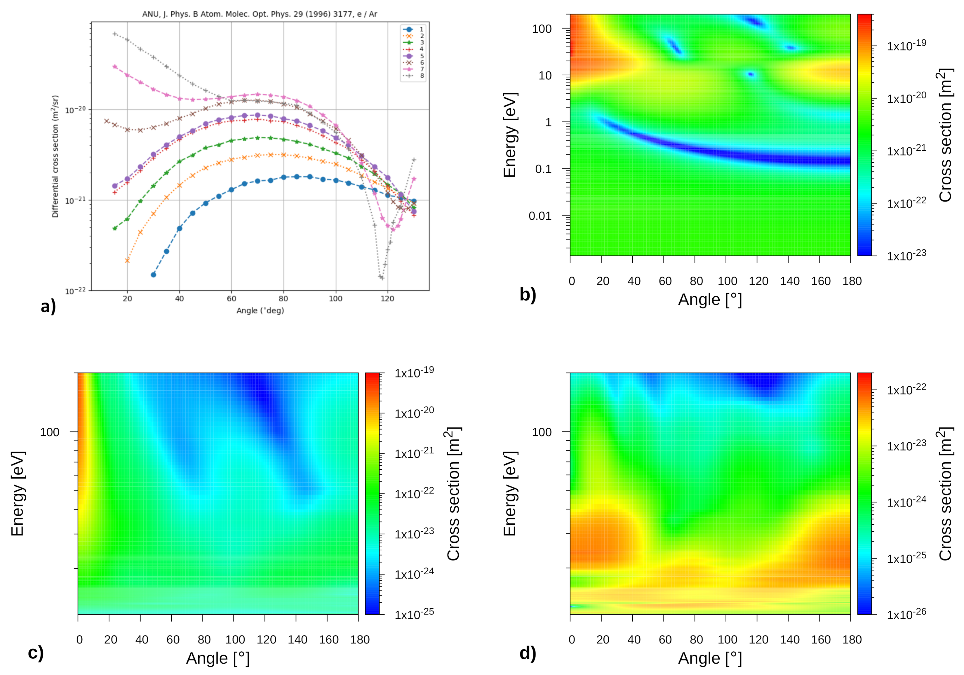
| 4.1.1 | Differential Scattering Cross-Sections ....................................................................................................... | 12 | ||
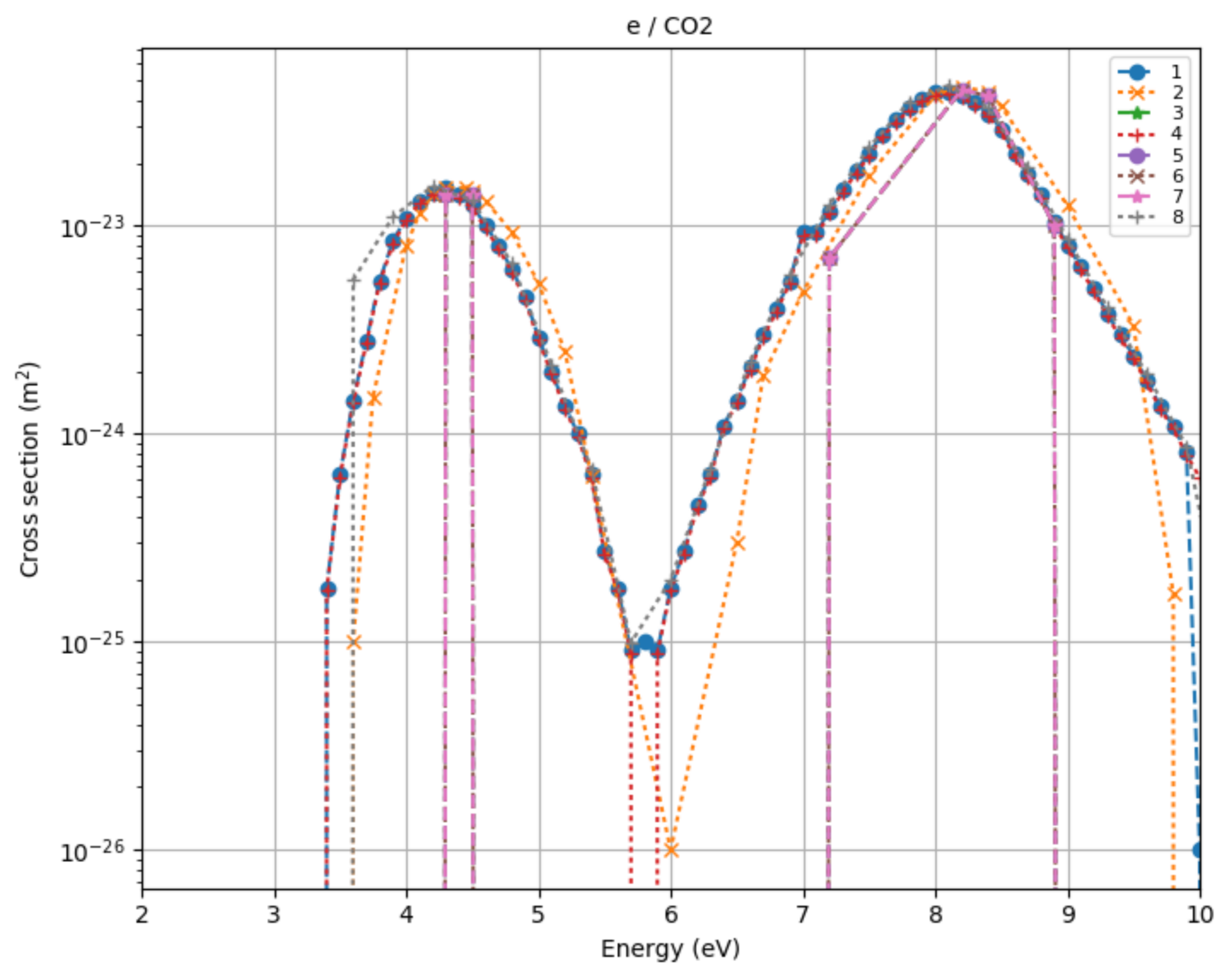
| 4.1.2 | Electron-Scattering Cross-Sections ............................................................................................................ | 12 | ||
| 4.1.3 | Swarm/Transport Data for Electrons ......................................................................................................... | 14 | ||
| 4.1.4 | Ion-Scattering Cross-Sections ..................................................................................................................... | 16 | ||
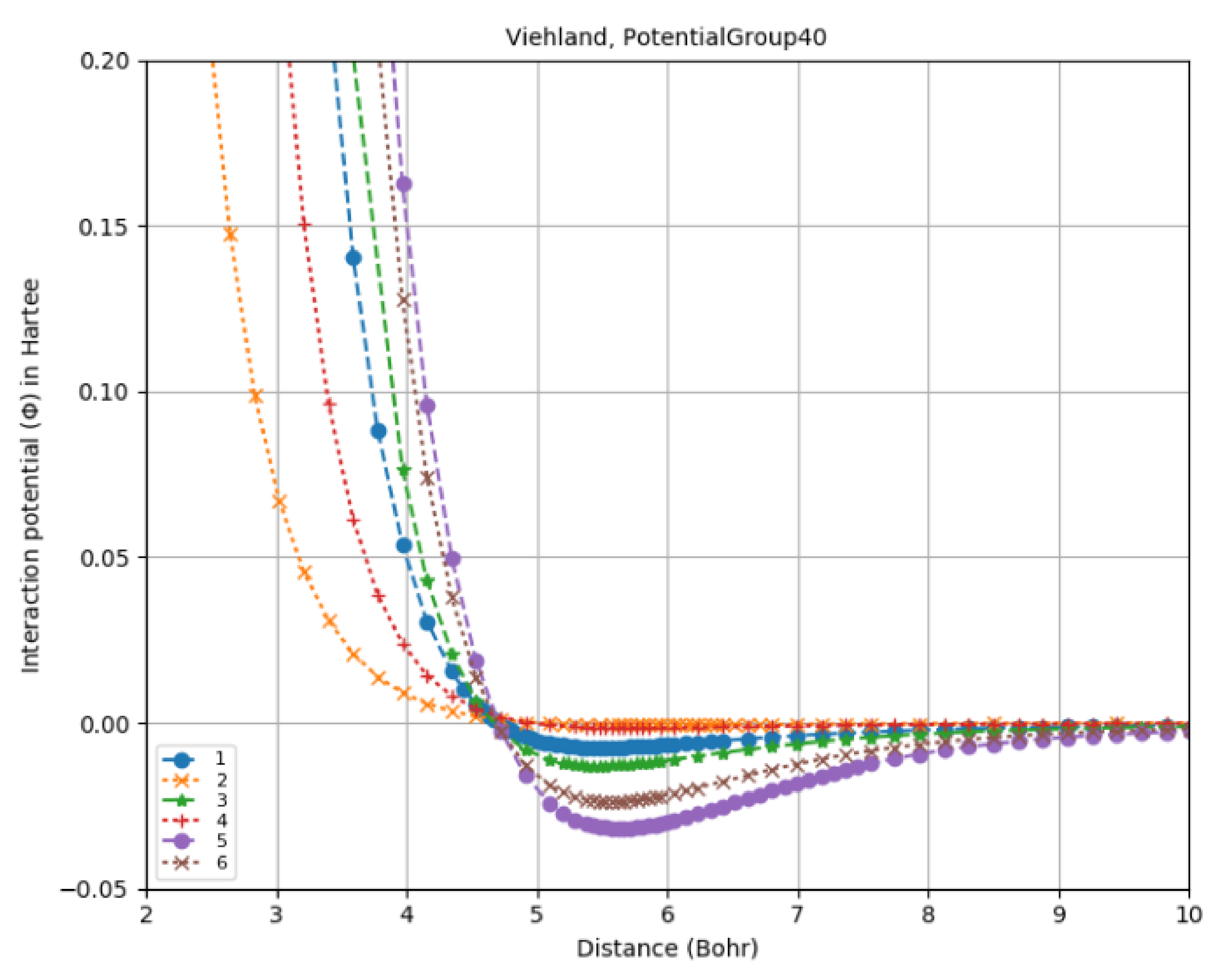
| 4.1.5 | Interaction Potentials ................................................................................................................................... | 17 | ||
| 4.1.6 | Swarm/Transport Data for Ions .................................................................................................................. | 18 | ||
| 4.2 | List of Species ........................................................................................................................................................... | 19 | ||
| 4.3 | Staging Areas on LXCat .......................................................................................................................................... | 19 | ||
| 5 | Tutorial: Online Calculations, Data Retrieval and Use | 21 | ||
| 5.1 | Video Tutorial .......................................................................................................................................................... | 21 | ||
| 5.2 | Comparison of Data ................................................................................................................................................ | 21 | ||
| 5.3 | LXCat Online Boltzmann Solver and Swarm Parameters Comparison ............................................................ | 22 | ||
| 5.4 | Definitions, Guidelines, and Best Practices .......................................................................................................... | 24 | ||
| 6 | LXCat under the Hood | 27 | ||
| 6.1 | The Exchange Format and Choice for a Database Type ..................................................................................... | 28 | ||
| 6.2 | Framework Implementation .................................................................................................................................. | 30 | ||
| 6.3 | Afternote .................................................................................................................................................................. | 30 | ||
| 7 | Recent Developments and Perspectives | 31 | ||
| 8 | Conclusions | 32 | ||
| A | How to Cite Data Retrieved from LXCat and Online Calculations | 33 | ||
| B | Referencing and Redistribution of Data | 33 | ||
| References | 34 | |||
1. Introduction
The integrity of the results obtained from numerical modeling depends […] on the identification of a physical model appropriate for addressing the problem of interest, on a good choice and proper implementation of the numerical solution techniques, and on the availability of reliable input data.
Apart from the obvious advantages that open data could bring for reproducibility and scientific integrity–although there is devil in the detail of how to implement this–one argument in favour of data sharing is that having more pairs of eyes on data may lead to new discoveries and faster scientific progress.
2. Data Needs for Modeling LTPs
2.1. Kinetic Models: Cross-Sections
2.2. Fluid Models: Transport Coefficients and Reaction Rate Coefficients
2.3. Additional Needs for Modeling Non-Equilibrium Plasmas
3. History and Statistics
3.1. Origins
3.2. LXCat 10 Years Later
3.3. Data for Modeling of Plasmas (DMP) Association
- encourage the exchange and open access of fundamental data via the Internet;
- develop tools to facilitate the exchange of online data;
- contribute to the collection and evaluation of data;
- communicate with the international scientific community to increase the visibility of fundamental data available online;
- communicate with specialists via forums such as the French Cold Plasma Network;
- encourage open access to numerical tools for the generation and analysis of data as well as for modeling plasmas;
- contribute to the standardization of formats for storing and exchange of data.
4. What Is Available on LXCat?
4.1. List of Data Groups, Databases and Species
4.1.1. Differential Scattering Cross-Sections
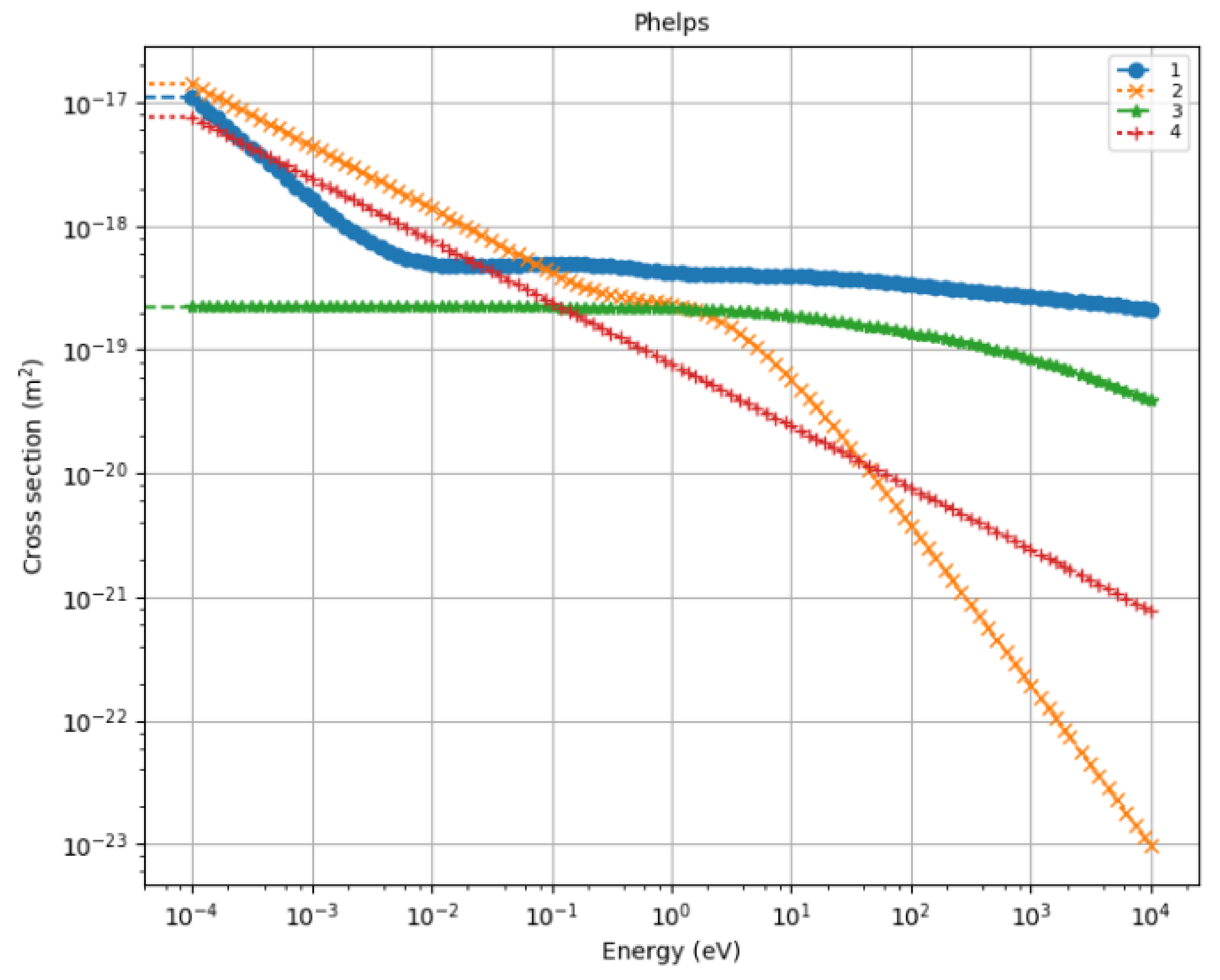
4.1.2. Electron-Scattering Cross-Sections
- Elastic: elastic momentum-transfer process.
- Excitation: electron-scattering process where part of its kinetic energy is transferred into electronic excitation of atoms or molecules. Similarly, excitation of rotational and vibrational levels of molecules are electron-impact excitation processes.
- Ionization: ionization process, inelastic collision in which a new electron is created.
- Attachment: an electron is lost in the collisional process. This can be either due to formation of negative ions but also electron-ion recombination.
- Effective: momentum transfer including all electron-scattering with a given target particle species. This is equal to the sum of the elastic momentum transfer and the total cross-sections for all inelastic and ionization processes. For historical reasons, this is included instead of elastic momentum transfer in some data sets.
- Biagi [80]: data transcribed by the LXCat team from S.F. Biagi’s FORTRAN code, MagBoltz, versions 8.9 and later [81,82], the exact version depending on the species as listed in the database. The database contains cross-sections for rare gases He, Ne, Ar, Kr, and Xe, and molecules H2, D2, N2, O2, CO2 and SF6. The transcription of data for other gases is in progress. These data were compiled for use with a Monte Carlo simulation (or multi-term Boltzmann code), but their use in a 2-term Boltzmann solver gives reasonably accurate results in most cases. Please note that the LXCat data tables do not have the same energy grid as the original data in the MagBoltz code.
- Biagi-v7.1 [83]: This database contains cross-sections for the rare gases He, Ne, Ar, Kr, and Xe, transcribed by the LXCat team from the Magboltz code version 7.1 by Stephen Biagi [81,82]. The excitation cross-sections are grouped into a few effective excitation levels. These cross-sections were compiled for use in a Monte Carlo (or multi-term Boltzmann) code.
- BSR [43]: The results in this database are from a semi-relativistic Breit-Pauli B-spline R-matrix (close-coupling) calculations [41,42]. It contains data for the species Ne, Ar, Kr, Xe, Be, C, N and F. Compared to 2016 the Ar data were extended with 469 records [87] and Be (201 records), C [88] (1178 records), N [89] (353 records), and F [90] (384 records) were added.
- FLINDERS [99]: A compilation of cross-sections uploaded to LXCat by Laurence Campbell of Flinders University, containing data for the species CO2, N2, NO, and O2.
- Hayashi [100]: These data sets were derived by comparing calculated swarm parameters, using as input the cross-sections sets in this database, with measurements. It contains data for the species Ar, Xe, C2H2, C2H4, C2H6, CCl2F2, CCl4, CF4, CH4, CO2, H2O, HCl, N2O, NH3, NO, Si2H6, SiH4, and SO2.
- IST-Lisbon [35]: This database contains data compiled from the literature from different authors, resulting in complete sets of cross-sections, validated against measured swarm parameters by solving the two-term homogeneous electron Boltzmann equation [101]. To improve predictions at low E/N, some sets need to be completed with rotational cross-sections, also available in the database. The following species are represented: He (replaced since 2016 [102]), Ar, CH4, H, H2, N (replaced since 2016 [103]), N2, O2, and added since 2016: CO [104], CO2 [105], O [106], and O2 vibrational states [107].
- Morgan (Kinema Research & Software) [110]: Cross-section sets suited for use with 2-term Boltzmann solvers assembled by W.L. Morgan for the species He, Ne, Ar, Xe, Kr, C, C2H2, C2H4, C2H6, C3H8, CF4, CH, CH2, CH3, CH4, Cl2, CO, CO2, F2, H, H2, H2O, HCl, N, N2, NH3, NO, O, O2, O3, SF6, and SiH4.
- NGFSRDW [111]: A set of excitation cross-section to individual fine-structure levels of Ar and Kr (a collection of 148 records added since 2016) calculated by Al Stauffer and co-workers.
- Phelps [112]: A compilation of atomic and molecular data, assembled and evaluated by A.V. Phelps and collaborators, including the species He, Ne, Ar, Xe, CO, CO2, H2, H2O, Mg, N2, Na, NO, O2, and SF6.
- Puech [113]: Cross-section sets assembled by V. Puech and colleagues in late 1980s and 1990s for the species Ne, Ar, Xe, C2H4, and C3H6.
- QUANTEMOL [114]: Data calculated and published by Quantemol Ltd. and associated researchers using Quantemol-N software/expert system [115]. This database includes the species BF3, C2, C2H2, C2OH6, C3, C3H4, C3N, CaF, CF, CF2, CF4, CH, CH4, CNH, CO, CO2, CONH3, COS, CS, F2O, H2, H2O, H2S, CH4, HBr, HCHO, HCN, HCP, Kr, N2, N2O, NH3, NO2, O2, O3, PH3, SiF2, SiH4, SiO, and SO2.
- SIGLO [116]: A compilation of data used in-house by the group GREPHE at LAPLACE in Toulouse, taken from different sources and including the species He, Ne, Ar, Xe, Kr, Cl2, CO2, Cu, F2, HCl, Hg, N2, SF6, and SiH4.
- TRINITI [117]: Cross-sections retrieved from the EEDF software package for calculations of the electron energy distribution function [118], for the species He, Ne, Ar, Xe, BCl, BCl2, BCl3, CF3I, CF4, CH4, CO, CO2, Cs, F2, H, H2, H2O, HCl, N2, Na, NF3, O, O2, and SF6. All data except O2 have been uploaded to LXCat since 2016.
4.1.3. Swarm/Transport Data for Electrons
- ETHZ [134]: Data obtained with pulsed Townsend experiments at the High Voltage Laboratory of ETH Zurich, Switzerland. It contains data for the species Ar, CO2, N2, and the gas mixtures 2−C4F8 with Ar, CO2, and N2, and c-C4F8O with Ar, CO2, and N2. Since 2016 the following species and gas mixtures have been added: CO2 (second set) [135], O2 [136], CH3CN, N2O [137], C3HF5 [138], C4F7N [139], C5F10O [140], SF5CF3 [141], CF3−O−CF=CF2, HFC227ea [142], HFO1234ze [143], and the gas mixtures C3HF5 with CO2 and N2 [138], C4F7N with CO2, CO2:O2, and N2 [139,144], C5F10O with CO2, CO2:O2, N2, and N2:O2 [140], CO2 with N2 and O2 [145], HFC227ea with CO2 and N2 [142], HFO1234ze with Ar, CO2, N2, and SF6 [143,146,147], HFPO with CO2 and N2 [148], N2:O2 [136], SF5CF3 with CO2 and N2 [141].
- LAPLACE [149]: Collection of data from after 1975 or not appearing in the Dutton compilation [133] digitized by S. Chowdhury from LAPLACE, Toulouse. It includes the gases Ar, C2F6, C2H4, C2H6, C3F8, C3H6 (cyclopropane and propene), C3H8, CF3I, CF4, CH4, CHF3, CO, CO2, H2, H2O, He, Kr, n-C4F10, N2, N2O, Ne, O2, Xe, Air, and the gas mixtures Air:H2O, CO2:Ar, H2:Ne, He:H2, N2:Ar, N2O:Ar, O2:Ar, Xe:H2, and Xe:N2.
- UNAM [150]: Electron-swarm data derived from pulsed Townsend experiments for the gases Ar, C2F4, C2F6, CF3I, CHF3, CO2, N2, SF6, and gas mixtures C2F4 with Ar and Xe, C2F6 with Ar and N2, CF3I with N2 and SF6, CHF3 with Ar and N2, and SF6 with Ar, CF4, CHF3, CO2, He, N2, N2O, O2, and Xe.
- CDAP (State-to-state electron-impact excitation rate coefficients) [151]: State-to-state electron-impact excitation rate coefficients between argon neutral or xenon ionic states obtained by combination of plasma experiments and theoretical calculations. In particular, the data are used for collisional-radiative modeling and examined in the afterglow plasma of argon (CDAP method) or examined in the different regions of electric propulsion devices using xenon. Rate coefficients for both atoms and ions are given here, and can be used for plasma modeling and optical emission spectroscopy (OES) [152,153].
- Heidelberg [154]: database of electron transport parameters measured at the University of Heidelberg in the years 1978 to 1996. Different electron-swarm experiments were setup by Bernhard Schmidt and co-workers which allowed to measure electron transport parameters in pure electric and perpendicular crossed electric and magnetic fields. This database contains only those data for B=0. Additional swarm data for non-zero B fields will be made available in tabular and graphical form when resources become available. The following gases and gas mixtures are present: C2H4, C2H6, C2H6O, C3H6, C3H8, CH4, CO2, D2, H2, N2, Ar:C2H6O, C4H10:Ar, C4H10:He, CO2:Ar, CO2:Ne, H2:Ar, H2:Kr, H2:Xe, and N2:Ar. These data were collected by Malte Hildebrandt, presently at the Paul Scherrer Institute in Switzerland, from publications and theses in the Heidelberg group and were made available to the LXCat team for inclusion in LXCat.
4.1.4. Ion-Scattering Cross-Sections
4.1.5. Interaction Potentials
4.1.6. Swarm/Transport Data for Ions
4.2. List of Species
4.3. Staging Areas on LXCat
- BOLSIG+ is a user-friendly Windows application for the numerical solution of he Boltzmann equation for electrons in weakly ionized gases in uniform electric fields, conditions which typically appear in the bulk of collisional low-temperature plasmas. Under these conditions the electron energy distribution is determined by the balance between acceleration in the electric field and momentum and energy loss in collisions with neutral gas particles [27,179]. An improved description of Coulomb collisions was developed by Hagelaar and is included in the more recent versions of BOLSIG+ [180].
- ZDPlasKin: Zero-Dimensional Plasma Kinetics solver ZDPlasKin is a Fortran 90 module designed to follow the time evolution of the species densities and gas temperature in a non-thermal plasma with an arbitrarily complex chemistry [21]. BOLSIG+ is integrated in this package.
- EEDF is a user-friendly program for the numerical solution of Boltzmann equation for the Electron Energy Distribution Function in low-ionized plasma in an electric field. It is used for calculations of electron transport and kinetic coefficients in gas mixtures. EEDF comes with Data Bank, several files containing data on cross-sections for the electron-scattering from atoms and molecules [118] compatible with EEDF program. These cross-section data can be found in the TRINITI database on LXCat.
- BOLOS: This package provides a pure Python library for the solution of the Boltzmann equation for electrons in a non-thermal plasma. It is a multi-platform, open-source implementation compatible with the LXCat cross-section input format [181].
- PumpKin: (pathway reduction method for plasma kinetic models) is a tool for post-processing of results from zero-dimensional plasma kinetics solvers. The goal is to analyze the production and/or destruction mechanisms of selected species of interest, as well as to reduce complex plasma chemistry models. Only once the user is required to solve first the full chemical reaction system. The output is then used as an input for PumpKin. The PumpKin package analyzes the full chemical reaction system, and automatically determines all significant pathways in the system, i.e., all pathways with a rate above a user-specified threshold [182,183].
- METHES is an open-source Monte Carlo collision code written in MATLAB for the simulation of electron transport in arbitrary gas mixtures in the presence of electric fields. For steady-state electron transport in a uniform electric field, the program provides the transport coefficients, reaction rates and the electron energy distribution function. The program is compatible with the electron-scattering cross-section files from LXCat. Temporal studies of electron transport are possible by tracking position, velocity and number of electrons [184,185].
- MultiBolt is a multi-term Boltzmann equation model for calculating electron kinetic phenomena in electron swarms and low-temperature plasmas. MultiBolt uses a combined electron density gradient and spherical harmonics decomposition of the electron phase space in the Boltzmann equation. From this, macroscopic rate and transport coefficients (flux and bulk) are calculated. MultiBolt has been demonstrated to be consistent with other popular kinetic models (BOLSIG+, METHES, and others), and is also in excellent agreement with other published models when calculating rate and transport coefficients for model gases, such as the Reid ramp model gas and the Lucas-Saelee attachment-ionization model gas. See also, J. Stephens, “A multi-term Boltzmann equation benchmark of electron-argon cross-sections for use in low-temperature plasma models” [186].
- LoKI-B: The LisbOn KInetics Boltzmann solver (LoKI-B), available as MATLAB open-source tool, solves the time and space independent form of the two-term electron Boltzmann equation, for non-magnetized non-equilibrium low-temperature plasmas excited by DC/HF electric fields from different gases or gas mixtures, considering growth models for the electron density to describe non-conservative events. LoKI-B can easily simulate the electron kinetics in any complex gas mixture (of atomic/molecular species), describing first and second-kind electron collisions with any target state (electronic, vibrational and rotational), characterized by any user-prescribed population [187].
- THERMCAT: A fast and robust online tool for simulation of different modes of axially symmetric current transfer from high-pressure arc-discharge plasmas to cylindrical thermionic cathodes, created and maintained by Mikhail Benilov and co-workers. The code computes both the diffuse mode of current transfer and modes with axially symmetric spots and can be used in a wide range of arc currents, plasma-producing gases, and cathode materials and dimensions. The tool also serves as a tutorial that can help to make physicists and engineers working in the field comfortable with multiple solutions describing different modes of current transfer to electrodes in low-temperature plasmas [188,189].
- ELEM: A code for evaluation of the field to thermo-field to thermionic electron emission current density. The code is based on an accurate and computationally efficient method of evaluation of the Murphy-Good formalism [190].
- MOBION: A code for evaluation of the mobility and temperature of ions in a weakly ionized gas as functions of reduced electric field and gas temperature. The code is based on the two-temperature displaced-distribution theory [191].
5. Tutorial: Online Calculations, Data Retrieval and Use
5.1. Video Tutorial
5.2. Comparison of Data
5.3. LXCat Online Boltzmann Solver and Swarm Parameters Comparison
5.4. Definitions, Guidelines, and Best Practices
- Historical origins of electron-neutral cross-section sets
- Definition of complete set
- Mixing cross-sections data sets or using incomplete sets
- Selection of a cross-sections data set
- The elastic momentum-transfer cross-section and anisotropic scattering
- Swarm configurations and growth models
- Piecewise linear interpolation of cross-sections
- Bulk and flux transport coefficients
- Temperature range for validity of a given set of cross-sections
- Treatment of three-body collisions
- Sorting and filtering target species
- Accessing and viewing large data sets online
- Chemistry models and how they affect calculations
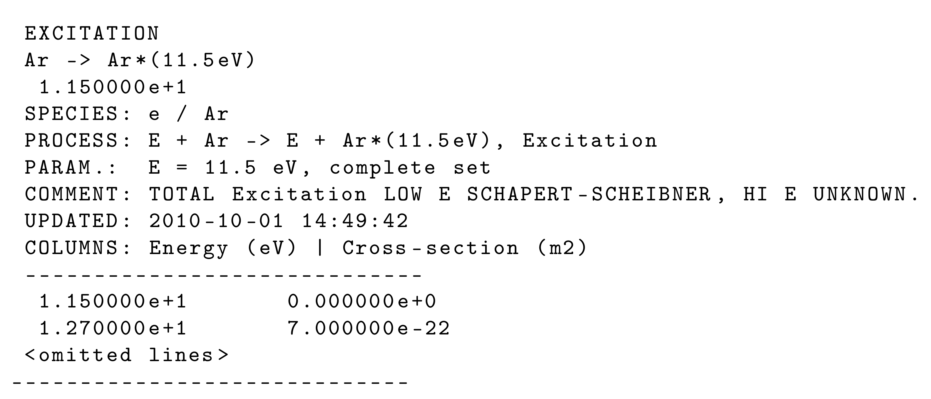
- Formatting for excitation and superelastic processes in a cross-section file
6. LXCat under the Hood
- The data exchange format, the data model and the choice for a database type;
- The overall framework design.
6.1. The Exchange Format and Choice for a Database Type
6.2. Framework Implementation
6.3. Afternote
7. Recent Developments and Perspectives
8. Conclusions
Author Contributions
Funding
Acknowledgments
Conflicts of Interest
Appendix A. How to Cite Data Retrieved from LXCat and Online Calculations
Appendix B. Referencing and Redistribution of Data
- Third parties should direct their users to the LXCat website to obtain data. Before downloading data, visitors to the site are asked to click to confirm that “Yes. I understand the LXCat policy and I agree to properly reference these data”. The header in downloaded files contains reference information that should be included in all publications making use of LXCat data and further guidelines for proper referencing are given in Appendix A.
- The LXCat team can provide customized interfaces to institutional members of the non-profit association “Data for Modeling Plasmas” (http://assoc.lxcat.net). This option is useful for code developers who recommend specific LXCat data sets for use in their software; that is, users who access the LXCat website through such a customized interface are directed to the specific data chosen by the code developers.
- In cases where neither of the above options is practical, third parties can include data from LXCat in their packages under the following conditions:
- Explicit written permission must be obtained from the owner of the database (the contributor) whose data is being included in the third-party package.
- LXCat must be notified in advance and a Memorandum Of Understanding (MOU) must be prepared between the LXCat team, the contributors who agree to have their data set redistributed within a software or any other shareable format and the MOU must be signed by all parties.
- A statement must be clearly visible with the redistributed data saying that “The data were downloaded from [database name], www.lxcat.net, [retrieval date]. LXCat is an open-access website with databases contributed by members of the scientific community.”.
- All output files generated by a third-party software when using data from LXCat must include in the header the reference “[database name], www.lxcat.net, [retrieval date]” and all other references supplied by the contributors as included in the headers of files downloaded from LXCat.
References
- Samukawa, S.; Hori, M.; Rauf, S.; Tachibana, K.; Bruggeman, P.; Kroesen, G.; Whitehead, J.C.; Murphy, A.B.; Gutsol, A.F.; Starikovskaia, S.; et al. The 2012 Plasma Roadmap. J. Phys. D Appl. Phys. 2012, 45, 253001. [Google Scholar] [CrossRef]
- Bekeschus, S.; Favia, P.; Robert, E.; von Woedtke, T. White paper on plasma for medicine and hygiene: Future in plasma health sciences. Plasma Process. Polym. 2019, 16, 1800033. [Google Scholar] [CrossRef] [Green Version]
- Brandenburg, R.; Bogaerts, A.; Bongers, W.; Fridman, A.; Fridman, G.; Locke, B.R.; Miller, V.; Reuter, S.; Schiorlin, M.; Verreycken, T.; et al. White paper on the future of plasma science in environment, for gas conversion and agriculture. Plasma Process. Polym. 2019, 16, 1700238. [Google Scholar] [CrossRef] [Green Version]
- Starikovskaia, S.M. Plasma assisted ignition and combustion. J. Phys. D Appl. Phys. 2006, 39, R265–R299. [Google Scholar] [CrossRef]
- Whitehead, J.C. Plasma–catalysis: The known knowns, the known unknowns and the unknown unknowns. J. Phys. D Appl. Phys. 2016, 49, 243001. [Google Scholar] [CrossRef]
- Pitchford, L.C.; Alves, L.L.; Bartschat, K.; Biagi, S.F.; Bordage, M.C.; Phelps, A.V.; Ferreira, C.M.; Hagelaar, G.J.M.; Morgan, W.L.; Pancheshnyi, S.; et al. Comparisons of sets of electron–neutral scattering cross sections and swarm parameters in noble gases: I. Argon. J. Phys. D Appl. Phys. 2013, 46, 334001. [Google Scholar] [CrossRef]
- Petrović, Z.L.; Dujko, S.; Marić, D.; Malović, G.; Nikitović, Ž.; Šašić, O.; Jovanović, J.; Stojanović, V.; Radmilović-Rađenović, M. Measurement and interpretation of swarm parameters and their application in plasma modelling. J. Phys. D Appl. Phys. 2009, 42, 194002. [Google Scholar] [CrossRef]
- Pitchford, L.C. GEC Plasma Data Exchange Project. J. Phys. D Appl. Phys. 2013, 46, 330301. [Google Scholar] [CrossRef]
- Alves, L.L.; Bartschat, K.; Biagi, S.F.; Bordage, M.C.; Pitchford, L.C.; Ferreira, C.M.; Hagelaar, G.J.M.; Morgan, W.L.; Pancheshnyi, S.; Phelps, A.V.; et al. Comparisons of sets of electron–neutral scattering cross sections and swarm parameters in noble gases: II. Helium and neon. J. Phys. D Appl. Phys. 2013, 46, 334002. [Google Scholar] [CrossRef]
- Bordage, M.C.; Biagi, S.F.; Alves, L.L.; Bartschat, K.; Chowdhury, S.; Pitchford, L.C.; Hagelaar, G.J.M.; Morgan, W.L.; Puech, V.; Zatsarinny, O. Comparisons of sets of electron–neutral scattering cross sections and swarm parameters in noble gases: III. Krypton and xenon. J. Phys. D Appl. Phys. 2013, 46, 334003. [Google Scholar] [CrossRef]
- Bartschat, K. Computational methods for electron–atom collisions in plasma applications. J. Phys. D Appl. Phys. 2013, 46, 334004. [Google Scholar] [CrossRef]
- Bertolotti, J. One size doesn’t fit all. Nat. Phys. 2019, 15, 724. [Google Scholar] [CrossRef] [Green Version]
- Zatsarinny, O.; Bartschat, K. The B-spline R-matrix method for atomic processes: Application to atomic structure, electron collisions and photoionization. J. Phys. At. Mol. Opt. Phys. 2013, 46, 112001. [Google Scholar] [CrossRef]
- Biberman, L.M.; Vorob’ev, V.S.; Yakubov, I.T. Low-temperature plasmas with nonequilibrium ionization. Sov. Phys. Uspekhi 1979, 22, 411–432. [Google Scholar] [CrossRef]
- Editorial. A problem shared is a problem halved. Nat. Phys. 2019, 15, 107. [Google Scholar] [CrossRef]
- Raizer, Y.P.; Allen, J.E. Gas Discharge Physics; Springer: Berlin, Germany, 1997; Volume 2. [Google Scholar]
- Boulos, M.I. Thermal plasma processing. IEEE Trans. Plasma Sci. 1991, 19, 1078–1089. [Google Scholar] [CrossRef]
- Große-Kreul, S.; Hübner, S.; Benedikt, J.; von Keudell, A. Sampling of ions at atmospheric pressure: Ion transmission and ion energy studied by simulation and experiment. Eur. Phys. J. 2016, 70, 103. [Google Scholar] [CrossRef]
- Donnelly, V.M.; Kornblit, A. Plasma etching: Yesterday, today, and tomorrow. J. Vac. Sci. Technol. A 2013, 31, 050825. [Google Scholar] [CrossRef] [Green Version]
- Bruggeman, P.J.; Iza, F.; Brandenburg, R. Foundations of atmospheric pressure non-equilibrium plasmas. Plasma Sources Sci. Technol. 2017, 26, 123002. [Google Scholar] [CrossRef] [Green Version]
- Pancheshnyi, S.; Eismann, B.; Hagelaar, G.J.M.; Pitchford, L.C. Computer Code ZDPlasKin; University of Toulouse, LAPLACE, CNRS-UPS-INP: Toulouse, France, 2008; Available online: http://www.zdplaskin.laplace.univ-tlse.fr/ (accessed on 4 July 2020).
- Hurlbatt, A.; Gibson, A.R.; Schröter, S.; Bredin, J.; Foote, A.P.S.; Grondein, P.; O’Connell, D.; Gans, T. Concepts, Capabilities, and Limitations of Global Models: A Review. Plasma Process. Polym. 2017, 14, 1600138. [Google Scholar] [CrossRef] [Green Version]
- Janssen, J.F.J.; Pitchford, L.C.; Hagelaar, G.J.M.; van Dijk, J. Evaluation of angular scattering models for electron-neutral collisions in Monte Carlo simulations. Plasma Sources Sci. Technol. 2016, 25, 055026. [Google Scholar] [CrossRef]
- Surendra, M.; Graves, D.B.; Jellum, G.M. Self-consistent model of a direct-current glow discharge: Treatment of fast electrons. Phys. Rev. A 1990, 41, 1112–1125. [Google Scholar] [CrossRef]
- Alves, L.L.; Bogaerts, A.; Guerra, V.; Turner, M.M. Foundations of modelling of nonequilibrium low-temperature plasmas. Plasma Sources Sci. Technol. 2018, 27, 023002. [Google Scholar] [CrossRef]
- Longo, S. Monte Carlo models of electron and ion transport in non-equilibrium plasmas. Plasma Sources Sci. Technol. 2000, 9, 468–476. [Google Scholar] [CrossRef]
- Hagelaar, G.J.M.; Pitchford, L.C. Solving the Boltzmann equation to obtain electron transport coefficients and rate coefficients for fluid models. Plasma Sources Sci. Technol. 2005, 14, 722–733. [Google Scholar] [CrossRef]
- Viehland, L.A.; Mason, E. Gaseous lon mobility in electric fields of arbitrary strength. Ann. Phys. 1975, 91, 499–533. [Google Scholar] [CrossRef]
- Viehland, L.A.; Mason, E. Gaseous ion mobility and diffusion in electric fields of arbitrary strength. Ann. Phys. 1978, 110, 287–328. [Google Scholar] [CrossRef]
- Richards, A.D.; Thompson, B.E.; Sawin, H.H. Continuum modeling of argon radio frequency glow discharges. Appl. Phys. Lett. 1987, 50, 492–494. [Google Scholar] [CrossRef]
- Boeuf, J.P.; Pitchford, L.C. Two-dimensional model of a capacitively coupled rf discharge and comparisons with experiments in the Gaseous Electronics Conference reference reactor. Phys. Rev. E 1995, 51, 1376–1390. [Google Scholar] [CrossRef]
- Atanasova, M.; Carbone, E.A.D.; Mihailova, D.; Benova, E.; Degrez, G.; van der Mullen, J.J.A.M. Modelling of an RF plasma shower. J. Phys. D Appl. Phys. 2012, 45, 145202. [Google Scholar] [CrossRef]
- Koelman, P.; Heijkers, S.; Tadayon Mousavi, S.; Graef, W.; Mihailova, D.; Kozak, T.; Bogaerts, A.; van Dijk, J. A Comprehensive Chemical Model for the Splitting of CO2 in Non-Equilibrium Plasmas. Plasma Process. Polym. 2017, 14, 1600155. [Google Scholar] [CrossRef]
- Bílek, P.; Obrusník, A.; Hoder, T.; Šimek, M.; Bonaventura, Z. Electric field determination in air plasmas from intensity ratio of nitrogen spectral bands: II. Reduction of the uncertainty and state-of-the-art model. Plasma Sources Sci. Technol. 2018, 27, 085012. [Google Scholar] [CrossRef]
- IST-Lisbon Database. Available online: https://www.lxcat.net/IST-Lisbon (accessed on 5 December 2020).
- Adamovich, I.; Baalrud, S.D.; Bogaerts, A.; Bruggeman, P.J.; Cappelli, M.; Colombo, V.; Czarnetzki, U.; Ebert, U.; Eden, J.G.; Favia, P.; et al. The 2017 Plasma Roadmap: Low temperature plasma science and technology. J. Phys. D Appl. Phys. 2017, 50, 323001. [Google Scholar] [CrossRef]
- Pancheshnyi, S.; Biagi, S.; Bordage, M.; Hagelaar, G.; Morgan, W.; Phelps, A.; Pitchford, L. The LXCat project: Electron scattering cross sections and swarm parameters for low temperature plasma modeling. Chem. Phys. 2012, 398, 148–153. [Google Scholar] [CrossRef]
- Pitchford, L.C.; Alves, L.L.; Bartschat, K.; Biagi, S.F.; Bordage, M.C.; Bray, I.; Brion, C.E.; Brunger, M.J.; Campbell, L.; Chachereau, A.; et al. LXCat: An Open-Access, Web-Based Platform for Data Needed for Modeling Low Temperature Plasmas. Plasma Process. Polym. 2017, 14, 1600098. [Google Scholar] [CrossRef]
- Gibson, J.C.; Gulley, R.J.; Sullivan, J.P.; Buckman, S.J.; Chan, V.; Burrow, P.D. Elastic electron scattering from argon at low incident energies. J. Phys. B At. Mol. Opt. Phys. 1996, 29, 3177–3195. [Google Scholar] [CrossRef]
- ANU Database. Available online: www.lxcat.net (accessed on 7 November 2020).
- Zatsarinny, O.; Bartschat, K. B-spline Breit–Pauli R-matrix calculations for electron collisions with argon atoms. J. Phys. B At. Mol. Opt. Phys. 2004, 37, 4693–4706. [Google Scholar] [CrossRef]
- Allan, M.; Zatsarinny, O.; Bartschat, K. Near-threshold absolute angle-differential cross sections for electron-impact excitation of argon and xenon. Phys. Rev. A 2006, 74, 030701. [Google Scholar] [CrossRef] [Green Version]
- BSR Database. Available online: https://www.lxcat.net/BSR (accessed on 4 December 2020).
- Bray, I.; Stelbovics, A.T. Convergent close-coupling calculations of electron-hydrogen scattering. Phys. Rev. A 1992, 46, 6995–7011. [Google Scholar] [CrossRef] [Green Version]
- Fursa, D.V.; Bray, I. Calculation of electron-helium scattering. Phys. Rev. A 1995, 52, 1279–1297. [Google Scholar] [CrossRef]
- Zammit, M.C.; Fursa, D.V.; Bray, I. Electron scattering from the molecular hydrogen ion and its isotopologues. Phys. Rev. A 2014, 90, 022711. [Google Scholar] [CrossRef]
- Zammit, M.C.; Savage, J.S.; Fursa, D.V.; Bray, I. Complete Solution of Electronic Excitation and Ionization in Electron-Hydrogen Molecule Scattering. Phys. Rev. Lett. 2016, 116, 233201. [Google Scholar] [CrossRef] [Green Version]
- Christophorou, L.G.; Olthoff, J.K. Electron Interactions with SF6. J. Phys. Chem. Ref. Data 2000, 29, 267–330. [Google Scholar] [CrossRef] [Green Version]
- Christophorou, L.G.; Olthoff, J.K. Electron Interactions with CF3I. J. Phys. Chem. Ref. Data 2000, 29, 553–569. [Google Scholar] [CrossRef]
- Zawadzki, M.; Wright, R.; Dolmat, G.; Martin, M.F.; Diaz, B.; Hargreaves, L.; Coleman, D.; Fursa, D.V.; Zammit, M.C.; Scarlett, L.H.; et al. Low-energy electron scattering from molecular hydrogen: Excitation of the to transition. Phys. Rev. A 2018, 98, 062704. [Google Scholar] [CrossRef] [Green Version]
- Brunger, M.J.; Buckman, S.J.; Allen, L.J.; McCarthy, I.E.; Ratnavelu, K. Elastic electron scattering from helium: Absolute experimental cross sections, theory and derived interaction potentials. J. Phys. B At. Mol. Opt. Phys. 1992, 25, 1823–1838. [Google Scholar] [CrossRef]
- Gulley, R.J.; Alle, D.T.; Brennan, M.J.; Brunger, M.J.; Buckman, S.J. Differential and total electron scattering from neon at low incident energies. J. Phys. B At. Mol. Opt. Phys. 1994, 27, 2593–2611. [Google Scholar] [CrossRef]
- Cho, H.; Gulley, R.J.; Buckman, S. Elastic Electron Scattering from Krypton at Backward Angles. J. Korean Phys. Soc. 2003, 42, 71–75. [Google Scholar]
- Cho, H.; McEachran, R.P.; Tanaka, H.; Buckman, S.J. The role of absorption in intermediate energy elastic electron scattering from krypton. J. Phys. B At. Mol. Opt. Phys. 2004, 37, 4639–4645. [Google Scholar] [CrossRef]
- Gibson, J.C.; Lun, D.R.; Allen, L.J.; McEachran, R.P.; Parcell, L.A.; Buckman, S.J. Low-energy electron scattering from xenon. J. Phys. B At. Mol. Opt. Phys. 1998, 31, 3949–3964. [Google Scholar] [CrossRef]
- Francis-Staite, J.R.; Maddern, T.M.; Brunger, M.J.; Buckman, S.J.; Winstead, C.; McKoy, V.; Bolorizadeh, M.A.; Cho, H. Differential and integral cross sections for elastic electron scattering from CF2. Phys. Rev. A 2009, 79, 052705. [Google Scholar] [CrossRef]
- Bundschu, C.T.; Gibson, J.C.; Gulley, R.J.; Brunger, M.J.; Buckman, S.J.; Sanna, N.; Gianturco, F.A. Low-energy electron scattering from methane. J. Phys. B At. Mol. Opt. Phys. 1997, 30, 2239–2259. [Google Scholar] [CrossRef]
- Panajotovic, R.; Jelisavcic, M.; Kajita, R.; Tanaka, T.; Kitajima, M.; Cho, H.; Tanaka, H.; Buckman, S.J. Electron scattering from tetrafluoroethylene. J. Chem. Phys. 2004, 121, 4559–4569. [Google Scholar] [CrossRef] [PubMed]
- Panajotovic, R.; Kitajima, M.; Tanaka, H.; Jelisavcic, M.; Lower, J.; Campbell, L.; Brunger, M.J.; Buckman, S.J. Electron collisions with ethylene. J. Phys. B At. Mol. Opt. Phys. 2003, 36, 1615–1626. [Google Scholar] [CrossRef]
- Jelisavcic, M.; Panajotovic, R.; Kitajima, M.; Hoshino, M.; Tanaka, H.; Buckman, S.J. Electron scattering from perfluorocyclobutane (c−C4F8). J. Chem. Phys. 2004, 121, 5272–5280. [Google Scholar] [CrossRef]
- Colyer, C.J.; Vizcaino, V.; Sullivan, J.P.; Brunger, M.J.; Buckman, S.J. Absolute elastic cross-sections for low-energy electron scattering from tetrahydrofuran. New J. Phys. 2007, 9, 41. [Google Scholar] [CrossRef]
- Vizcaino, V.; Roberts, J.; Sullivan, J.P.; Brunger, M.J.; Buckman, S.J.; Winstead, C.; McKoy, V. Elastic electron scattering from 3-hydroxytetrahydrofuran: Experimental and theoretical studies. New J. Phys. 2008, 10, 053002. [Google Scholar] [CrossRef]
- Gulley, R.J.; Buckman, S.J. Absolute elastic electron scattering from benzene. J. Phys. B At. Mol. Opt. Phys. 1999, 32, L405–L409. [Google Scholar] [CrossRef]
- Cho, H.; Gulley, R.J.; Sunohara, K.; Kitajima, M.; Uhlmann, L.J.; Tanaka, H.; Buckman, S.J. Elastic electron scattering from C6H6 and C6F6. J. Phys. B At. Mol. Opt. Phys. 2001, 34, 1019–1038. [Google Scholar] [CrossRef]
- Gibson, J.C.; Morgan, L.A.; Gulley, R.J.; Brunger, M.J.; Bundschu, C.T.; Buckman, S.J. Low energy electron scattering from CO: Absolute cross section measurements and R-matrix calculations. J. Phys. B At. Mol. Opt. Phys. 1996, 29, 3197–3214. [Google Scholar] [CrossRef]
- Gibson, J.C.; Green, M.A.; Trantham, K.W.; Buckman, S.J.; Teubner, P.J.O.; Brunger, M.J. Elastic electron scattering from CO2. J. Phys. B At. Mol. Opt. Phys. 1999, 32, 213–233. [Google Scholar] [CrossRef]
- Cho, H.; Gulley, R.J.; Trantham, K.W.; Uhlmann, L.J.; Dedman, C.J.; Buckman, S.J. Elastic electron scattering from sulfur hexafluoride. J. Phys. B At. Mol. Opt. Phys. 2000, 33, 3531–3544. [Google Scholar] [CrossRef]
- Brunger, M.J.; Buckman, S.J.; Newman, D.S.; Alle, D.T. Elastic scattering and rovibrational excitation of H2 by low-energy electrons. J. Phys. B At. Mol. Opt. Phys. 1991, 24, 1435–1448. [Google Scholar] [CrossRef]
- Cho, H.; Park, Y.S.; Tanaka, H.; Buckman, S.J. Measurements of elastic electron scattering by water vapour extended to backward angles. J. Phys. B At. Mol. Opt. Phys. 2004, 37, 625–634. [Google Scholar] [CrossRef]
- Gulley, R.J.; Brunger, M.J.; Buckman, S.J. The scattering of low energy electrons from hydrogen sulphide. J. Phys. B At. Mol. Opt. Phys. 1993, 26, 2913–2925. [Google Scholar] [CrossRef]
- Vizcaino, V.; Jelisavcic, M.; Sullivan, J.P.; Buckman, S.J. Elastic electron scattering from formic acid (HCOOH): Absolute differential cross-sections. New J. Phys. 2006, 8, 85. [Google Scholar] [CrossRef]
- Sullivan, J.P.; Gibson, J.C.; Gulley, R.J.; Buckman, S.J. Low-energy electron scattering from O2. J. Phys. B At. Mol. Opt. Phys. 1995, 28, 4319–4328. [Google Scholar] [CrossRef]
- Brennan, M.J.; Alle, D.T.; Euripides, P.; Buckman, S.J.; Brunger, M.J. Elastic electron scattering and rovibrational excitation of N2 at low incident energies. J. Phys. B At. Mol. Opt. Phys. 1992, 25, 2669–2682. [Google Scholar] [CrossRef]
- Sun, W.; Morrison, M.A.; Isaacs, W.A.; Trail, W.K.; Alle, D.T.; Gulley, R.J.; Brennan, M.J.; Buckman, S.J. Detailed theoretical and experimental analysis of low-energy electron-N2 scattering. Phys. Rev. A 1995, 52, 1229–1256. [Google Scholar] [CrossRef] [PubMed]
- Kitajima, M.; Sakamoto, Y.; Gulley, R.J.; Hoshino, M.; Gibson, J.C.; Tanaka, H.; Buckman, S.J. Electron scattering from N2O: Absolute elastic scattering and vibrational excitation. J. Phys. B At. Mol. Opt. Phys. 2000, 33, 1687–1702. [Google Scholar] [CrossRef]
- Alle, D.T.; Gulley, R.J.; Buckman, S.J.; Brunger, M.J. Elastic scattering of low-energy electrons from ammonia. J. Phys. B At. Mol. Opt. Phys. 1992, 25, 1533–1542. [Google Scholar] [CrossRef]
- Gulley, R.J.; Brunger, M.J.; Buckman, S.J. Resonant excitation of NH3 by low energy electron impact: The ν1,3 normal vibrational modes. J. Phys. B At. Mol. Opt. Phys. 1992, 25, 2433–2440. [Google Scholar] [CrossRef]
- Mojarrabi, B.; Gulley, R.J.; Middleton, A.G.; Cartwright, D.C.; Teubner, P.J.O.; Buckman, S.J.; Brunger, M.J. Electron collisions with NO: Elastic scattering and rovibrational (0 to 1, 2, 3, 4) excitation cross sections. J. Phys. B At. Mol. Opt. Phys. 1995, 28, 487–504. [Google Scholar] [CrossRef]
- Gulley, R.J.; Buckman, S.J. Elastic scattering of low energy electrons from sulphur dioxide. J. Phys. B At. Mol. Opt. Phys. 1994, 27, 1833–1843. [Google Scholar] [CrossRef]
- Biagi Database. Available online: www.lxcat.net/Biagi (accessed on 4 July 2020).
- Magboltz. Available online: https://magboltz.web.cern.ch/magboltz/ (accessed on 4 July 2020).
- Biagi, S. Monte Carlo simulation of electron drift and diffusion in counting gases under the influence of electric and magnetic fields. Nucl. Instrum. Methods Phys. Res. Sect. A Accel. Spectrometers Detect. Assoc. Equip. 1999, 421, 234–240. [Google Scholar] [CrossRef]
- Biagi v7.1 Database. Available online: https://www.lxcat.net/Biagi-v7.1 (accessed on 24 November 2020).
- Bordage Database. Available online: https://www.lxcat.net/Bordage (accessed on 24 November 2020).
- Segur, P.; Yousfi, M.; Kadri, M.H.; Bordage, M.C. A survey of the numerical methods currently in use to describe the motion of an electron swarm in a weakly ionized gas. Transp. Theory Stat. Phys. 1986, 15, 705–757. [Google Scholar] [CrossRef]
- Segur, P.; Bordage, M. Recent advances in the solution of the Boltzmann equation for the motion of electrons in a weakly ionized gas. In Proceedings of the 19th International Conference on Phenomena in Ionized Gases, Belgrade, Yugoslavia, 10–14 July 1989; pp. 86–107. [Google Scholar]
- Zatsarinny, O.; Wang, Y.; Bartschat, K. Electron-impact excitation of argon at intermediate energies. Phys. Rev. A 2014, 89, 022706. [Google Scholar] [CrossRef]
- Wang, Y.; Zatsarinny, O.; Bartschat, K. B-spline R-matrix-with-pseudostates calculations for electron-impact excitation and ionization of carbon. Phys. Rev. A 2013, 87, 012704. [Google Scholar] [CrossRef] [Green Version]
- Gedeon, V.; Gedeon, S.; Lazur, V.; Nagy, E.; Zatsarinny, O.; Bartschat, K. B-spline R-matrix-with-pseudostates calculations for electron-impact excitation and ionization of fluorine. Phys. Rev. A 2014, 89, 052713. [Google Scholar] [CrossRef]
- Wang, Y.; Zatsarinny, O.; Bartschat, K. B-spline R-matrix-with-pseudostates calculations for electron-impact excitation and ionization of nitrogen. Phys. Rev. A 2014, 89, 062714. [Google Scholar] [CrossRef]
- CCC Database. Available online: https://www.lxcat.net/CCC (accessed on 4 December 2020).
- Zammit, M.C.; Savage, J.S.; Fursa, D.V.; Bray, I. Electron-impact excitation of molecular hydrogen. Phys. Rev. A 2017, 95, 022708. [Google Scholar] [CrossRef] [Green Version]
- Scarlett, L.H.; Tapley, J.K.; Fursa, D.V.; Zammit, M.C.; Savage, J.S.; Bray, I. Low-energy electron-impact dissociative excitation of molecular hydrogen and its isotopologues. Phys. Rev. A 2017, 96, 062708. [Google Scholar] [CrossRef] [Green Version]
- Scarlett, L.H.; Tapley, J.K.; Fursa, D.V.; Zammit, M.C.; Savage, J.S.; Bray, I. Electron-impact dissociation of molecular hydrogen into neutral fragments. Eur. Phys. J. D 2018, 72, 1–8. [Google Scholar] [CrossRef]
- Christophorou Database. Available online: https://www.lxcat.net/Christophorou (accessed on 24 November 2020).
- COP Database. Available online: https://www.lxcat.net/COP (accessed on 24 November 2020).
- McEachran, R.; Stauffer, A. Momentum transfer cross sections for the heavy noble gases. Eur. Phys. J. D 2014, 68, 153. [Google Scholar] [CrossRef]
- McEachran, R.P.; Stauffer, A.D. Viscosity cross sections for the heavy noble gases. Eur. Phys. J. D 2015, 69, 106. [Google Scholar] [CrossRef]
- FLINDERS Database. Available online: https://www.lxcat.net/FLINDERS (accessed on 7 November 2020).
- Hayashi Database. Available online: https://www.lxcat.net/Hayashi (accessed on 24 November 2020).
- Alves, L.L. The IST-LISBON database on LXCat. J. Phys. Conf. Ser. 2014, 565, 012007. [Google Scholar] [CrossRef]
- Santos, M.; Noël, C.; Belmonte, T.; Alves, L.L. Microwave capillary plasmas in helium at atmospheric pressure. J. Phys. D Appl. Phys. 2014, 47, 265201. [Google Scholar] [CrossRef]
- Coche, P.; Guerra, V.; Alves, L.L. Microwave air plasmas in capillaries at low pressure I. Self-consistent modeling. J. Phys. D Appl. Phys. 2016, 49, 235207. [Google Scholar] [CrossRef]
- Ogloblina, P.; del Caz, A.T.; Guerra, V.; Alves, L.L. Electron impact cross sections for carbon monoxide and their importance in the electron kinetics of CO2–CO mixtures. Plasma Sources Sci. Technol. 2020, 29, 015002. [Google Scholar] [CrossRef]
- Grofulović, M.; Alves, L.L.; Guerra, V. Electron-neutral scattering cross sections for CO2: A complete and consistent set and an assessment of dissociation. J. Phys. D Appl. Phys. 2016, 49, 395207. [Google Scholar] [CrossRef]
- Alves, L.L.; Coche, P.; Ridenti, M.A.; Guerra, V. Electron scattering cross sections for the modelling of oxygen-containing plasmas. Eur. Phys. J. D 2016, 70, 124. [Google Scholar] [CrossRef]
- Annušová, A.; Marinov, D.; Booth, J.P.; Sirse, N.; da Silva, M.L.; Lopez, B.; Guerra, V. Kinetics of highly vibrationally excited O2(X) molecules in inductively-coupled oxygen plasmas. Plasma Sources Sci. Technol. 2018, 27, 045006. [Google Scholar] [CrossRef]
- Itikawa Database. Available online: https://www.lxcat.net/Itikawa (accessed on 24 November 2020).
- Itikawa, Y. Cross sections for electron collisions with nitric oxide. J. Phys. Chem. Ref. Data 2016, 45, 033106. [Google Scholar] [CrossRef]
- Morgan Database. Available online: https://www.lxcat.net/Morgan (accessed on 4 December 2020).
- NGFSRDW Database. Available online: https://www.lxcat.net/NGFSRDW (accessed on 24 November 2020).
- Phelps Database. Available online: https://www.lxcat.net/Phelps (accessed on 21 November 2020).
- Puech Database. Available online: https://www.lxcat.net/Puech (accessed on 24 November 2020).
- QUANTEMOL Database. Available online: https://www.lxcat.net/QUANTEMOL (accessed on 24 November 2020).
- QUANTEMOL. Available online: http://quantemol.com (accessed on 24 November 2020).
- SIGLO Database. Available online: https://www.lxcat.net/SIGLO (accessed on 24 November 2020).
- TRINITI Database. Available online: https://www.lxcat.net/TRINITI (accessed on 24 November 2020).
- Dyatko, N.; Kochetov, I.; Napartovich, A.; Sukharev, A. EEDF: The Software Package for Calculations of the Electron Energy Distribution Function in Gas Mixtures. Available online: http://www.lxcat.net/software/EEDF/ (accessed on 4 July 2020).
- UBC Database. Available online: https://www.lxcat.net/UBC (accessed on 26 November 2020).
- Drawin, H.W. Atomic Cross-Sections for Inelastic Electronic Collisions; Report EUR-CEA-FC 236; Association Euratom-CEA: Cadarache, France, 1963. [Google Scholar]
- Kim, Y.K. Scaled Born cross sections for excitations of H2 by electron impact. J. Chem. Phys. 2007, 126, 064305. [Google Scholar] [CrossRef] [PubMed]
- Kawahara, H.; Kato, H.; Hoshino, M.; Tanaka, H.; Brunger, M.J. Excitation of the C1Σ+ + c3Π and E1Π electronic states of carbon monoxide by electron impact. Phys. Rev. A 2008, 77, 012713. [Google Scholar] [CrossRef] [Green Version]
- Holland, D.M.P.; Shaw, D.A. A study of the valence shell absolute photoabsorption, photoionization and photodissociation cross sections, and the photoionization quantum efficiency of carbon monoxide. J. Phys. B At. Mol. Opt. Phys. 2020, 53, 144004. [Google Scholar] [CrossRef]
- eMol-LeHavre Database. Available online: https://www.lxcat.net/eMol-LeHavre (accessed on 27 November 2020).
- Laporta Database. Available online: https://www.lxcat.net/Laporta (accessed on 27 November 2020).
- Little, D.A.; Chakrabarti, K.; Mezei, J.Z.; Schneider, I.F.; Tennyson, J. Dissociative recombination of N2+: An ab initio study. Phys. Rev. A 2014, 90, 052705. [Google Scholar] [CrossRef] [Green Version]
- Pop, N.; Iacob, F.; Mezei, J.Z.; Motapon, O.; Niyonzima, S.; Kashinski, D.O.; Talbi, D.; Hickman, A.P.; Schneider, I.F. Reactive collisions of electrons with H2+, HD+, BeH+, BeD+ and SH+. AIP Conf. Proc. 2017, 1916, 020013. [Google Scholar] [CrossRef]
- Niyonzima, S.; Ilie, S.; Pop, N.; Mezei, J.Z.; Chakrabarti, K.; Morel, V.; Peres, B.; Little, D.; Hassouni, K.; Larson, Å.; et al. Low-energy collisions between electrons and BeH+: Cross sections and rate coefficients for all the vibrational states of the ion. At. Data Nucl. Data Tables 2017, 115–116, 287–308. [Google Scholar] [CrossRef] [Green Version]
- Laporta, V.; Tennyson, J.; Schneider, I.F. Vibrationally resolved NO dissociative excitation cross sections by electron impact. Plasma Sources Sci. Technol. 2020, 29, 05LT02. [Google Scholar] [CrossRef] [Green Version]
- Laporta, V.; Schneider, I.F.; Tennyson, J. Dissociative electron attachment cross sections for ro-vibrationally excited NO molecule and N-anion formation. Plasma Sources Sci. Technol. 2020, 29, 10LT01. [Google Scholar] [CrossRef]
- Laporta, V.; Celiberto, R.; Tennyson, J. Dissociative electron attachment and electron-impact resonant dissociation of vibrationally excited O2 molecules. Phys. Rev. A 2015, 91, 012701. [Google Scholar] [CrossRef] [Green Version]
- Dutton Database. Available online: https://www.lxcat.net/Dutton (accessed on 26 November 2020).
- Dutton, J. A survey of electron swarm data. J. Phys. Chem. Ref. Data 1975, 4, 577–856. [Google Scholar] [CrossRef]
- ETHZ Database. Available online: https://www.lxcat.net/ETHZ (accessed on 7 November 2020).
- Vass, M.; Egüz, E.; Chachereau, A.; Hartmann, P.; Korolov, I.; Hösl, A.; Bošnjaković, D.; Dujko, S.; Donkó, Z.; Franck, C.M. Electron transport parameters in CO2: A comparison of two experimental systems and measured data. J. Phys. D Appl. Phys. 2020, 54, 035202. [Google Scholar] [CrossRef]
- Haefliger, P.; Hösl, A.; Franck, C.M. Experimentally derived rate coefficients for electron ionization, attachment and detachment as well as ion conversion in pure O2 and N2–O2 mixtures. J. Phys. D Appl. Phys. 2018, 51, 355201. [Google Scholar] [CrossRef]
- Hösl, A.; Pachin, J.; Egüz, E.; Chachereau, A.; Franck, C.M. Measurement and modeling of electron and anion kinetics in N2O discharges. J. Phys. D Appl. Phys. 2020, 53, 135202. [Google Scholar] [CrossRef] [Green Version]
- Pachin, J.; Hösl, A.; Franck, C.M. Measurements of the electron swarm parameters of R1225ye(Z) (C3HF5) and its mixtures with N2 and CO2. J. Phys. D Appl. Phys. 2019, 52, 235204. [Google Scholar] [CrossRef] [Green Version]
- Chachereau, A.; Hösl, A.; Franck, C.M. Electrical insulation properties of the perfluoronitrile C4F7N. J. Phys. D Appl. Phys. 2018, 51, 495201. [Google Scholar] [CrossRef] [Green Version]
- Chachereau, A.; Hösl, A.; Franck, C.M. Electrical insulation properties of the perfluoroketone C5F10O. J. Phys. D Appl. Phys. 2018, 51, 335204. [Google Scholar] [CrossRef] [Green Version]
- Chachereau, A.; Franck, C.M. Measurement of the electron attachment properties of SF5CF3 and comparison to SF6. J. Phys. D Appl. Phys. 2017, 50, 445204. [Google Scholar] [CrossRef] [Green Version]
- Chachereau, A.; Franck, C. Electron swarm parameters of the hydrofluorocarbon HFC-227ea and its mixtures with N2 and CO2. In Proceedings of the 22nd International Conference on Gas Discharges and Their Applications (GD 2018), Novi Sad, Serbia, 2–7 September 2018. [Google Scholar]
- Chachereau, A.; Rabie, M.; Franck, C.M. Electron swarm parameters of the hydrofluoroolefine HFO1234ze. Plasma Sources Sci. Technol. 2016, 25, 045005. [Google Scholar] [CrossRef]
- Egüz, E.; Chachereau, A.; Hösl, A.; Franck, C. Measurements of Swarm Parameters in C4F7N: O2: CO2, C5F10O: O2: CO2 and C5F10O: O2: N2 Mixtures. In Proceedings of the 19th International Symposium on High Voltage Engineering (ISH 2019), Pilsen, Czech Republic, 23–28 August 2019. [Google Scholar]
- Haefliger, P.; Franck, C.M. Comparison of swarm and breakdown data in mixtures of nitrogen, carbon dioxide, argon and oxygen. J. Phys. D Appl. Phys. 2018, 52, 025204. [Google Scholar] [CrossRef] [Green Version]
- Chachereau, A.; Franck, C. Characterization of HFO1234ze mixtures with N2 and CO2 for use as gaseous electrical insulation media. In Proceedings of the 20th International Symposium on High Voltage Engineering (ISH 2017), Buenos Aires, Argentina, 28 August–1 September 2017; p. 257. [Google Scholar] [CrossRef]
- Hösl, A.; Pachin, J.; Egüz, E.; Chachereau, A.; Franck, C.M. Positive synergy of SF6 and HFO1234ze(E). IEEE Trans. Dielectr. Electr. Insul. 2020, 27, 322–324. [Google Scholar] [CrossRef] [Green Version]
- Zawadzki, M.; Chachereau, A.; Kočišek, J.; Franck, C.M.; Fedor, J. Electron attachment to hexafluoropropylene oxide (HFPO). J. Chem. Phys. 2018, 149, 204305. [Google Scholar] [CrossRef] [PubMed] [Green Version]
- LAPLACE Database. Available online: https://www.lxcat.net/LAPLACE (accessed on 21 November 2020).
- UNAM Database. Available online: www.lxcat.net/UNAM (accessed on 21 November 2020).
- CDAP Database. Available online: https://www.lxcat.net/CDAP (accessed on 26 November 2020).
- Zhu, X.M.; Wang, Y.F.; Wang, Y.; Yu, D.R.; Zatsarinny, O.; Bartschat, K.; Tsankov, T.V.; Czarnetzki, U. A xenon collisional-radiative model applicable to electric propulsion devices: II. Kinetics of the 6s, 6p, and 5d states of atoms and ions in Hall thrusters. Plasma Sources Sci. Technol. 2019, 28, 105005. [Google Scholar] [CrossRef]
- Zhu, X.M.; Cheng, Z.W.; Carbone, E.; Pu, Y.K.; Czarnetzki, U. Determination of state-to-state electron-impact rate coefficients between Ar excited states: A review of combined diagnostic experiments in afterglow plasmas. Plasma Sources Sci. Technol. 2016, 25, 043003. [Google Scholar] [CrossRef]
- Heidelberg Database. Available online: www.lxcat.net/Heidelberg (accessed on 21 November 2020).
- UT Database. Available online: https://www.lxcat.net/UT (accessed on 26 November 2020).
- Aints, M.; Jõgi, I.; Laan, M.; Paris, P.; Raud, J. Effective ionization coefficient of C5 perfluorinated ketone and its mixtures with air. J. Phys. D Appl. Phys. 2018, 51, 135205. [Google Scholar] [CrossRef]
- Phelps, A.V. The application of scattering cross sections to ion flux models in discharge sheaths. J. Appl. Phys. 1994, 76, 747–753. [Google Scholar] [CrossRef]
- Viehland Database. Available online: https://www.lxcat.net/Viehland (accessed on 26 November 2020).
- Viehland, L.A.; Kirkpatrick, C.C. Relating ion/neutral reaction rate coefficients and cross-sections by accessing a database for ion transport properties. Int. J. Mass Spectrom. Ion Process. 1995, 149-150, 555–571. [Google Scholar] [CrossRef]
- Qing, E.; Viehland, L.A.; Lee, E.P.F.; Wright, T.G. Interaction potentials and spectroscopy of Hg+ · Rg and Cd+ · Rg and transport coefficients for Hg+ and Cd+ in Rg (Rg = He − Rn). J. Chem. Phys. 2006, 124, 044316. [Google Scholar] [CrossRef] [PubMed] [Green Version]
- Basurto, E.; Urquijo, J.D. Mobility of CF3+ in CF4, CHF2+ in CHF3, and C+ in Ar. J. Appl. Phys. 2002, 91, 36–39. [Google Scholar] [CrossRef]
- Tuttle, W.D.; Thorington, R.L.; Viehland, L.A.; Wright, T.G. Interaction potentials, spectroscopy and transport properties of C+(2PJ) and C+(4PJ) with helium. Mol. Phys. 2015, 113, 3767–3782. [Google Scholar] [CrossRef]
- Tuttle, W.D.; Thorington, R.L.; Viehland, L.A.; Breckenridge, W.H.; Wright, T.G. Interactions of C+(2PJ) with rare gas atoms: Incipient chemical interactions, potentials and transport coefficients. Philos. Trans. R. Soc. Math. Phys. Eng. Sci. 2018, 376, 20170156. [Google Scholar] [CrossRef] [Green Version]
- von Helden, G.; Kemper, P.R.; Hsu, M.; Bowers, M.T. Determination of potential energy curves for ground and metastable excited state transition metal ions interacting with helium and neon using electronic state chromatography. J. Chem. Phys. 1992, 96, 6591–6605. [Google Scholar] [CrossRef]
- Buchachenko, A.A.; Viehland, L.A. Ab initio study of the mobility of Gd+ ions in He and Ar gases. Int. J. Mass Spectrom. 2019, 443, 86–92. [Google Scholar] [CrossRef]
- Galbis, E.; Douady, J.; Jacquet, E.; Giglio, E.; Gervais, B. Potential energy curves and spin-orbit coupling of light alkali-heavy rare gas molecules. J. Chem. Phys. 2013, 138, 014314. [Google Scholar] [CrossRef]
- Viehland, L.A.; Lozeille, J.; Soldán, P.; Lee, E.P.F.; Wright, T.G. Spectroscopy of K+ · Rg and transport coefficients of K+ in Rg (Rg = He − Rn). J. Chem. Phys. 2004, 121, 341–351. [Google Scholar] [CrossRef] [PubMed] [Green Version]
- Gardner, A.M.; Withers, C.D.; Graneek, J.B.; Wright, T.G.; Viehland, L.A.; Breckenridge, W.H. Theoretical Study of M+-RG and M2+-RG Complexes and Transport of M+ through RG (M = Be and Mg, RG = He − Rn). J. Phys. Chem. A 2010, 114, 7631–7641. [Google Scholar] [CrossRef] [PubMed]
- Tuttle, W.D.; Harris, J.P.; Zheng, Y.; Breckenridge, W.H.; Wright, T.G. Hybridization and Covalency in the Group 2 and Group 12 Metal Cation/Rare Gas Complexes. J. Phys. Chem. A 2018, 122, 7679–7703. [Google Scholar] [CrossRef] [PubMed]
- Allard, N.F.; Guillon, G.; Alekseev, V.A.; Kielkopf, J.F. Theoretical profiles of the Mg+ resonance lines perturbed by collisions with He. A&A 2016, 593, A13. [Google Scholar] [CrossRef] [Green Version]
- Bejaoui, M.; Dhiflaoui, J.; Mabrouk, N.; El Ouelhazi, R.; Berriche, H. Theoretical Investigation of the Electronic Structure and Spectra of Mg2+He and Mg+He. J. Phys. Chem. A 2016, 120, 747–753. [Google Scholar] [CrossRef] [PubMed]
- Viehland, L.A.; Webb, R.; Lee, E.P.; Wright, T.G. Accurate potential energy curves for HeO−, NeO−, and ArO−: Spectroscopy and transport coefficients. J. Chem. Phys. 2005, 122, 114302. [Google Scholar] [CrossRef] [Green Version]
- Garand, E.; Buchachenko, A.A.; Yacovitch, T.I.; Szczȩśniak, M.M.; Chałasiński, G.; Neumark, D.M. Study of KrO− and KrO via Slow Photoelectron Velocity-Map Imaging Spectroscopy and ab Initio Calculations. J. Phys. Chem. A 2009, 113, 14439–14446. [Google Scholar] [CrossRef] [Green Version]
- Wright, T.G.; Viehland, L.A. Accurate potential energy curves for HeS−: Spectroscopy and transport coefficients. Chem. Phys. Lett. 2006, 420, 24–28. [Google Scholar] [CrossRef]
- Tuttle, W.D.; Thorington, R.L.; Viehland, L.A.; Wright, T.G. Theoretical study of Si+(2PJ)–RG complexes and transport of Si+(2PJ) in RG (RG = He − Ar). Mol. Phys. 2017, 115, 437–446. [Google Scholar] [CrossRef] [Green Version]
- Viehland, L.A.; Gray, B.R.; Wright, T.G. Interaction potentials, spectroscopy and transport properties of RG+–He (RG = Ar − Rn). Mol. Phys. 2009, 107, 2127–2139. [Google Scholar] [CrossRef]
- Ellis, H.; Pai, R.; McDaniel, E.; Mason, E.; Viehland, L. Transport properties of gaseous ions over a wide energy range. At. Data Nucl. Data Tables 1976, 17, 177–210. [Google Scholar] [CrossRef]
- Viehland, L.; Mason, E. Transport Properties of Gaseous Ions over a Wide Energy Range, IV. At. Data Nucl. Data Tables 1995, 60, 37–95. [Google Scholar] [CrossRef]
- BOLSIG+. Version: 12/2017. Available online: http://www.bolsig.laplace.univ-tlse.fr/ (accessed on 8 December 2020).
- Hagelaar, G.J.M. Coulomb collisions in the Boltzmann equation for electrons in low-temperature gas discharge plasmas. Plasma Sources Sci. Technol. 2016, 25, 015015. [Google Scholar] [CrossRef] [Green Version]
- BOLOS. Available online: https://github.com/aluque/bolos/ (accessed on 4 July 2020).
- Markosyan, A.; Luque, A.; Gordillo-Vázquez, F.; Ebert, U. PumpKin: A tool to find principal pathways in plasma chemical models. Comput. Phys. Commun. 2014, 185, 2697–2702. [Google Scholar] [CrossRef] [Green Version]
- Markosyan, A.; Luque, A.; Gordillo-Vázquez, F.; Ebert, U. PumpKin: A Tool to Find Principal Pathways in Plasma Chemical Models. 2013. Available online: www.pumpkin-tool.org/ (accessed on 4 July 2020).
- Rabie, M.; Franck, C. METHES: A Monte Carlo collision code for the simulation of electron transport in low temperature plasmas. Comput. Phys. Commun. 2016, 203, 268–277. [Google Scholar] [CrossRef] [Green Version]
- Rabie, M.; Franck, C. METHES Code. 2015. Available online: www.lxcat.net/download/METHES/ (accessed on 4 July 2020).
- Stephens, J. A multi-term Boltzmann equation benchmark of electron-argon cross-sections for use in low temperature plasma models. J. Phys. D Appl. Phys. 2018, 51, 125203. [Google Scholar] [CrossRef]
- del Caz, A.T.; Guerra, V.; Gonçalves, D.; da Silva, M.L.; Marques, L.; Pinhão, N.; Pintassilgo, C.D.; Alves, L.L. The LisbOn KInetics Boltzmann solver. Plasma Sources Sci. Technol. 2019, 28, 043001. [Google Scholar] [CrossRef]
- Benilov, M.S.; Cunha, M.D.; Naidis, G.V. Modelling interaction of multispecies plasmas with thermionic cathodes. Plasma Sources Sci. Technol. 2005, 14, 517–524. [Google Scholar] [CrossRef] [Green Version]
- THERMCAT. Available online: http://www.arc_cathode.uma.pt (accessed on 4 July 2020).
- Benilov, M.S.; Benilova, L.G. Field to thermo-field to thermionic electron emission: A practical guide to evaluation and electron emission from arc cathodes. J. Appl. Phys. 2013, 114, 063307. [Google Scholar] [CrossRef]
- Almeida, P.G.C.; Benilov, M.S.; Naidis, G.V. Calculation of ion mobilities by means of the two-temperature displaced-distribution theory. J. Phys. D Appl. Phys. 2002, 35, 1577–1584. [Google Scholar] [CrossRef] [Green Version]
- Renda, M.; Ciubotaru, D.A. Betaboltz: A Monte-Carlo simulation tool for gas scattering processes. arXiv 2019, arXiv:1901.08140. [Google Scholar]
- Yamabe, C.; Buckman, S.J.; Phelps, A.V. Measurement of free-free emission from low-energy-electron collisions with Ar. Phys. Rev. A 1983, 27, 1345–1352. [Google Scholar] [CrossRef]
- Nakamura, Y.; Kurachi, M. Electron transport parameters in argon and its momentum transfer cross section. J. Phys. D Appl. Phys. 1988, 21, 718–723. [Google Scholar] [CrossRef]
- Kruithof, A. Townsend’s ionization coefficients for neon, argon, krypton and xenon. Physica 1940, 7, 519–540. [Google Scholar] [CrossRef]
- W.L. Morgan’s Compilation Database. Available online: http://www.kinema.com/download.htm (accessed on 4 July 2020).
- Stephens, J.C.; on behalf of the LXCat team. An Introduction to the LXCat Website. Available online: https://www.lxcat.net/tutorial (accessed on 8 December 2020).
- Biagi, S. Fortran Program, MAGBOLTZ v11.6.
- Bailey, V.; Rudd, J. CVI. The behaviour of electrons in nitrous oxide. Lond. Edinb. Dublin Philos. Mag. J. Sci. 1932, 14, 1033–1046. [Google Scholar] [CrossRef]
- Rees, J. Measurements of Townsend’s Energy Factor k1 for Electrons in Carbon Dioxide. Aust. J. Phys. 1964, 17, 462. [Google Scholar] [CrossRef] [Green Version]
- Schlumbohm, H. Stoßionisierungskoeffizient α, mittlere Elektronenenergien und die Beweglichkeit von Elektronen in Gasen. Z. Phys. 1965, 184, 492–505. [Google Scholar] [CrossRef]
- Schlumbohm, H. Messung der Driftgeschwindigkeiten von Elektronen und positiven Ionen in Gasen. Z. Phys. 1965, 182, 317–327. [Google Scholar] [CrossRef]
- Skinker, M. LXXXVIII. The motion of electrons in carbon dioxide. Lond. Edinb. Dublin Philos. Mag. J. Sci. 1922, 44, 994–999. [Google Scholar] [CrossRef] [Green Version]
- Wagner, E.; Davis, F.; Hurst, G. Time-of-Flight Investigations of Electron Transport in Some Atomic and Molecular Gases. J. Chem. Phys. 1967, 47, 3138–3147. [Google Scholar] [CrossRef]
- Warren, R.W.; Parker, J.H., Jr. Ratio of the Diffusion Coefficient to the Mobility Coefficient for Electrons in He, Ar, N2, H2, D2, CO, and CO2 at Low Temperatures and Low E/p. Phys. Rev. 1962, 128, 2661. [Google Scholar] [CrossRef]
- Fink, X.; Huber, P. Wanderungsgeschwindigkeit und Diffusionskonstante von Elektronen in Methan. Helv. Phys. Acta. 1965, 38, 717. [Google Scholar] [CrossRef]
- Elford, M. The drift velocity of electrons in carbon dioxide at 293 ∘K. Aust. J. Phys 1966, 19, 629. [Google Scholar]
- Frommhold, L. Eine untersuchung der elektronenkomponente von elektronenlawinen im homogenen feld II. Z. Phys. 1960, 160, 554–567. [Google Scholar] [CrossRef]
- Pack, J.; Voshall, R.; Phelps, A. Drift velocities of slow electrons in krypton, xenon, deuterium, carbon monoxide, carbon dioxide, water vapor, nitrous oxide, and ammonia. Phys. Rev. 1962, 127, 2084. [Google Scholar] [CrossRef]
- Haefliger, P.; Franck, C.M. Detailed precision and accuracy analysis of swarm parameters from a pulsed Townsend experiment. Rev. Sci. Instrum. 2018, 89, 023114. [Google Scholar] [CrossRef] [PubMed]
- Bortner, T.; Hurst, G.; Stone, W. Drift velocities of electrons in some commonly used counting gases. Rev. Sci. Instrum. 1957, 28, 103–108. [Google Scholar] [CrossRef]
- Elford, M.; Haddad, G. The drift velocity of electrons in carbon dioxide at temperatures between 193 and 573 K. Aust. J. Phys. 1980, 33, 517–530. [Google Scholar] [CrossRef] [Green Version]
- Nakamura, Y. Drift Velocity and Longitudinal Diffusion Coefficient of Electrons in CO2-Ar Mixtures and Electron Collision Cross Sections for CO2 Molecules. Aust. J. Phys. 1995, 48, 357–364, Digitized by H. Hasegawa 1994. [Google Scholar] [CrossRef] [Green Version]
- Roznerski, W.; Leja, K. Electron drift velocity in hydrogen, nitrogen, oxygen, carbon monoxide, carbon dioxide and air at moderate E/N. J. Phys. D Appl. Phys. 1984, 17, 279. [Google Scholar] [CrossRef]
- Bhalla, M.; Craggs, J. Measurement of ionization and attachment coefficients in carbon dioxide in uniform fields. Proc. Phys. Soc. 1960, 76, 369. [Google Scholar] [CrossRef]
- Conti, V.J.; Williams, A.W. Proceedings of the Eighth International Conference on Phenomena in Ionized Gases. Wien, Austria, 27 August–2 September 1967; Springer: Wien, Austria. Available online: https://0-www-springer-com.brum.beds.ac.uk/gp/book/9783709145227 (accessed on 23 February 2021).
- Hurst, H. Die Entstehung der Ionen durch Zusammenstoß und die Funkenspannung in Kohlendioxyd und Stickstoff. Phil. Mag 1906, 11, 535. [Google Scholar] [CrossRef] [Green Version]
- Schlumbohm, H. Elektronenlawinen in elektronegativen Gasen. Z. Phys. 1962, 166, 192–206. [Google Scholar] [CrossRef]
- Townsend, J.S. LXVI. The conductivity produced in gases by the aid of ultra-violet light. Lond. Edinb. Dublin Philos. Mag. J. Sci. 1902, 3, 557–576. [Google Scholar] [CrossRef] [Green Version]
- Phelps, A.V.; Pitchford, L.C. Anisotropic scattering of electrons by N2 and its effect on electron transport. Phys. Rev. A 1985, 31, 2932–2949. [Google Scholar] [CrossRef] [PubMed]
- Hagelaar, G.J.M. A new user-friendly Monte-Carlo based Boltzmann equation solver for weakly ionized gases. In Proceedings of the 73nd Gaseous Electronics Conference, Virtual Conference (Oral), San Diego, CA, USA, 5–9 October 2020. [Google Scholar]
- Kumar, K.; Skullerud, H.; Robson, R.E. Kinetic theory of charged particle swarms in neutral gases. Aust. J. Phys. 1980, 33, 343–448. [Google Scholar] [CrossRef] [Green Version]
- Carbone, E.A.D.; Schregel, C.G.; Czarnetzki, U. Ignition and afterglow dynamics of a high pressure nanosecond pulsed helium micro-discharge: II. Rydberg molecules kinetics. Plasma Sources Sci. Technol. 2016, 25, 054004. [Google Scholar] [CrossRef] [Green Version]
- Ventzek, P.; Hoekstra, R.; Kushner, M. Two-dimensional modeling of high plasma density inductively coupled sources for materials processing. J. Vac. Sci. Technol. B 1994, 12, 461–477. [Google Scholar] [CrossRef]
- van Dijk, J.; Peerenboom, K.; Jimenez, M.; Mihailova, D.; van der Mullen, J. The plasma modelling toolkit Plasimo. J. Phys. D Appl. Phys. 2009, 42, 194012. [Google Scholar] [CrossRef]
| 1 | As will be seen later, the velocity distribution function of electrons is frequently non-Maxwellian. However, the term ‘temperature’ is often used where ‘mean energy’ would be more appropriate. |
| 2 | |
| 3 | There exists also a second Townsend coefficient, characterizing the yield of electrons from a cathode bombarded by positive ions which helps sustaining a discharge. |
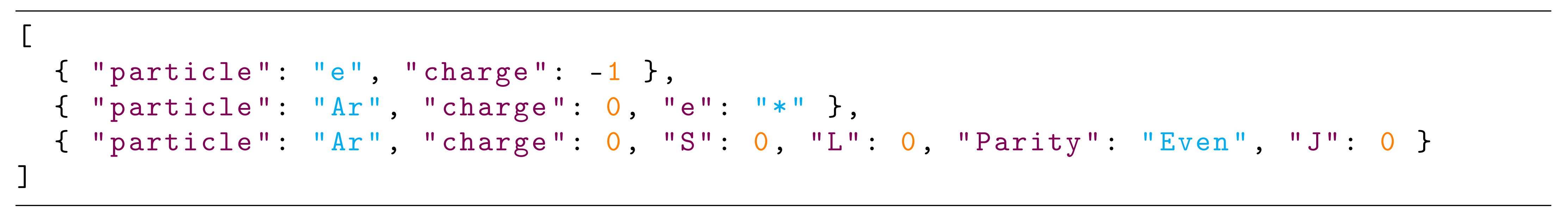
| 4 | For the interested reader: we have built a framework for the compilation of the schema files from elementary building blocks in JavaScript/TypeScript, which also can host chemical (non-electronic) processes in a future database release. |


| Particle | Charge | e | S | L | Parity | J |
|---|---|---|---|---|---|---|
| e | −1 | NULL | NULL | NULL | NULL | NULL |
| Ar | 0 | * | NULL | NULL | NULL | NULL |
| Ar | 0 | NULL | 0 | 0 | Even | 0 |
Publisher’s Note: MDPI stays neutral with regard to jurisdictional claims in published maps and institutional affiliations. |
© 2021 by the authors. Licensee MDPI, Basel, Switzerland. This article is an open access article distributed under the terms and conditions of the Creative Commons Attribution (CC BY) license (http://creativecommons.org/licenses/by/4.0/).
Share and Cite
Carbone, E.; Graef, W.; Hagelaar, G.; Boer, D.; Hopkins, M.M.; Stephens, J.C.; Yee, B.T.; Pancheshnyi, S.; van Dijk, J.; Pitchford, L. Data Needs for Modeling Low-Temperature Non-Equilibrium Plasmas: The LXCat Project, History, Perspectives and a Tutorial. Atoms 2021, 9, 16. https://0-doi-org.brum.beds.ac.uk/10.3390/atoms9010016
Carbone E, Graef W, Hagelaar G, Boer D, Hopkins MM, Stephens JC, Yee BT, Pancheshnyi S, van Dijk J, Pitchford L. Data Needs for Modeling Low-Temperature Non-Equilibrium Plasmas: The LXCat Project, History, Perspectives and a Tutorial. Atoms. 2021; 9(1):16. https://0-doi-org.brum.beds.ac.uk/10.3390/atoms9010016
Chicago/Turabian StyleCarbone, Emile, Wouter Graef, Gerjan Hagelaar, Daan Boer, Matthew M. Hopkins, Jacob C. Stephens, Benjamin T. Yee, Sergey Pancheshnyi, Jan van Dijk, and Leanne Pitchford. 2021. "Data Needs for Modeling Low-Temperature Non-Equilibrium Plasmas: The LXCat Project, History, Perspectives and a Tutorial" Atoms 9, no. 1: 16. https://0-doi-org.brum.beds.ac.uk/10.3390/atoms9010016