Article

Machine Learning Predictions of Transition Probabilities in Atomic Spectra

by
Joshua J. Michalenko
*,
Christopher M. Murzyn
,
Joshua D. Zollweg
,
Lydia Wermer
,
Alan J. Van Omen
and
Michael D. Clemenson
Sandia National Laboratories, Albuquerque, NM 87123, USA
*
Author to whom correspondence should be addressed.
Submission received: 22 October 2020 / Revised: 19 December 2020 / Accepted: 21 December 2020 / Published: 6 January 2021

Abstract

:
Forward modeling of optical spectra with absolute radiometric intensities requires knowledge of the individual transition probabilities for every transition in the spectrum. In many cases, these transition probabilities, or Einstein A-coefficients, quickly become practically impossible to obtain through either theoretical or experimental methods. Complicated electronic orbitals with higher order effects will reduce the accuracy of theoretical models. Experimental measurements can be prohibitively expensive and are rarely comprehensive due to physical constraints and sheer volume of required measurements. Due to these limitations, spectral predictions for many element transitions are not attainable. In this work, we investigate the efficacy of using machine learning models, specifically fully connected neural networks (FCNN), to predict Einstein A-coefficients using data from the NIST Atomic Spectra Database. For simple elements where closed form quantum calculations are possible, the data-driven modeling workflow performs well but can still have lower precision than theoretical calculations. For more complicated nuclei, deep learning emerged more comparable to theoretical predictions, such as Hartree–Fock. Unlike experiment or theory, the deep learning approach scales favorably with the number of transitions in a spectrum, especially if the transition probabilities are distributed across a wide range of values. It is also capable of being trained on both theoretical and experimental values simultaneously. In addition, the model performance improves when training on multiple elements prior to testing. The scalability of the machine learning approach makes it a potentially promising technique for estimating transition probabilities in previously inaccessible regions of the spectral and thermal domains on a significantly reduced timeline.

1. Introduction

Spectroscopic techniques can provide useful quantitative measurements across a variety of scientific disciplines. While broadly applicable, spectroscopic methods are often tailored to achieve a niche measurement. Therefore, data can be collected across a wide range of spectral resolutions, instrument parameters, excitation sources, temporal sampling rates, optical depths, and temperature variations. The high dimensional nature of this measurement space presents a challenge for implementing generalized analysis and forward modeling capability that is effective across all disciplines and experimental methods.
To augment expensive quantitative measurements, methods for simulating optical spectra are well documented in the scientific literature [1,2]. Utilizing forward modeling allows a simulated spectrum to be parametrically fit to measured data, thereby accounting for temperature and instrument effects using closed form equations and modest computational resources. In many cases, the primary limitation of forward spectral modeling is a lack of spectral constants available in the literature or spectral databases. These constants may not be available due to a lack of resources in the community, complexity in theoretical calculations, or the sheer volume of experiments required to produce the needed fundamental parameters.
Integral to any quantitative optical spectral model is the transition probability. The transition probability (a.k.a. Einstein coefficient, A-coefficient, oscillator strength, gf-value) is a temperature independent property representing the spontaneous emission rate in a two-level energy model. The pedagogy of both theoretical and experimental determination of transition probabilities is very rich, as the preferred methods of both areas have changed over time [3,4,5]. For the simplest nuclei, complete quantum mechanical calculations can yield nearly exact values more precise than any experiment [6,7,8]. For light elements, Hartree–Fock calculations are widely accepted theoretical treatments and yield accuracies comparable with experimental measurements [9,10,11,12,13,14]. Transition probabilities for heavy nuclei are derived almost entirely from experimental data and can have the largest uncertainties [15,16,17].
Machine learning (ML) has recently gained traction as a potential method to perform a generalized analysis of spectroscopic data [18,19,20,21,22] and there is some work published on predicting spectra using these methods [23]. Although efforts are being made to generalize spectral analysis with artificial intelligence [19,24], many approaches still implicitly reduce the dimensionality. For example, reduced generalization occurs for a model which only analyzes data collected with a single type of instrument and spectral resolution. Additionally, any variation in temperature or optical depth during an experiment can significantly alter an optical emission or absorption spectrum which may limit analytical performance of ML when applied more broadly than the specific training conditions. To overcome these hindrances to generalization, we hypothesize that neural network (NN) architectures can predict transition probabilities and can be coupled with closed-form, forward spectral modeling to more generically analyze and simulate optical spectra.

Contributions

This work examines a novel application of machine learning to spectroscopic data by implementing NN architectures trained on fundamental spectroscopic information to predict Einstein A-coefficients. We investigate if NNs can provide a method to estimate Einstein A-coefficient constants at a usable accuracy on a significantly shorter time scale relative to theoretical calculation or direct measurement. The general approach in this first-of-its-kind efficacy study is to predict Einstein A-coefficients for electronic transitions in atomic spectra by training NNs on published values of known spectral constants. In this way, the predictions of the neural network can be directly compared to data that are widely used by the community. This effort demonstrates a numeric encoding to represent spectroscopic transitions to be used by machine learning models followed by predictions of Einstein A-coefficients for various elements on the periodic table. The numeric dataset is built from the NIST Atomic Spectral Database (ASD) [25] as it is the paragon for tabulations of transition probabilities with bounded uncertainty, which allows us to assess the variance in the predictions produced by the neural network. In Section 2, we detail how NIST data are transformed into a machine-learnable format, followed by Section 3 where we describe experiment design and metrics used. A discussion of results including intraelement and interelement experiments, a direct comparison to previous theoretical work and model feature importance is presented in Section 4, followed by conclusions in Section 5.

2. Data Representation

Data representation in any machine learning model is arguably one of the most important design criteria. The data which is used to train the machine learning model must be provided to the model in a way that accurately preserves the most relevant information within the data [26]. Significant work in the field of cheminformatics has provided groundwork for presenting chemical and physical structure in representations interpretable by a NN [27,28,29]. Care must be taken in order to preserve the statistical characteristics (e.g., ordinal, categorical, boundedness) of each feature, or model input dimension, while providing a feature that can be interpreted by predictive models. The best possible set of features is the subset which preserves the most statistical information in the lowest possible dimension while contributing to model learning [30,31]. It is assumed in this focused work that feature representation of spectroscopic transitions would be intimately aligned with nuclear and electronic structural parameters as these are the fundamentals informing theoretical calculations [32]. In this section, we describe how the NIST tables of spectroscopic transitions are transformed into a ML-ready format.
The NIST ASD [25] contains a tabulated list of known, element-specific spectral transitions and transition probabilities per each element. For each tabulated spectral transition for a given element, we extracted from the NIST ASD the transition wavelength, the upper and lower state energy, the upper and lower state term symbol, the upper and lower electron configuration, the upper and lower degeneracy, the transition type (i.e., allowed or forbidden), and the transition probability. For a more detailed description of these parameters, the reader is directed to the NIST Atomic Spectroscopy compendium by Martin and Wiese [33].
As a data pre-processing step, we first strip away all transitions that do not have published A-coefficients since we cannot use them to train and evaluate our models. It is worth noting that a large set of transitions within each element do not have published Einstein coefficients but may be directly modeled using our approach subsequent to model training.
As it is standard in most machine learning pre-processing pipelines, we perform transformations on the data to create features and regressands that are well distributed [26]. Einstein A-coefficients, transition wavelength, and upper and lower energies typically range orders of magnitude across the various datasets. Such large variations in model features can create learning instabilities in the model. One mitigation strategy we employ is to transform these values with large dynamic ranges using log ( x + 1 ) . In this way, the widely ranging values are transformed to a scale that is more amenable to training while also avoiding undefined instances in the data. We additionally scale features by standardizing. Standardization scales model features to provide a data distribution with a mean of zero and a unit standard deviation. Standardization is a common ML practice as it is useful for improving algorithm stability [34]. However, standardizing data that is non-continuous (e.g., binary or categorical, such as the categories of “allowed” or “forbidden” transitions) must be performed with care. We encode these variables with a one-hot schema (−1/+1) to encourage symmetry about zero during rescaling. In this way, one category is designated numerically with a value of −1, while the other category is designated with a value of +1.
During our pre-processing, the type of transition (e.g., electric dipole, magnetic dipole, etc.) intuitively represents a valuable feature strongly influencing the transition probability. We initially labeled each transition type with a one-hot encoding scheme representing the type of transition covering all of the NIST-reported designations [35]. The NIST datasets are dominated by electronic dipole transitions to the point where most other transitions showed up as outliers in our trained models. Because of this, we elected to drop transitions other than electronic dipoles from the scope of this paper. This is also important as it removes the differing wavelength dependencies between line strength and A-coefficient across the various transition types (E1, M1, E2, etc.) [36,37]. We discuss how these transitions could be more accurately modeled in Section 4.
In the case of multiplet transitions with unresolved fine structure, tabulations include all of the allowable total angular momentum (J) values. From a data representation standpoint, those transitions are split up into otherwise identical transitions, each one having one of the allowable J values in the multiplet. This maintains a constant distribution over J values instead of introducing outlier features.

2.1. Electron Configuration

Quantum energy states with a defined electron configuration provide an opportunity to succinctly inform the model regarding wave function of the upper and lower states. This is arguably the most important feature as the configuration describes the wave functions which subsequently provide the overlap integral for the transition probability between two states [11,33,38]. We refer the reader to the text of Martin and Wiese [33] for more rigorous discussion of atomic states, quantum numbers, and multi-electron configurations.
Our encoding scheme for the electron configuration follows nl k nomenclature and represents each subshell with the principle quantum number (n) as well as the occupation number (k). For context in the present work, allowable values of n are positive integers, and l are integer values spaced by 1, ranging from 0 to n − 1. The variable l is represented in configurations with letters s, p, d, etc. denoting l = 0, 1, 2, etc. [33]. The reader is encouraged to find further information regarding electron configurations in the following references [33,38]. The orbital angular momentum quantum number (l) is represented through the feature’s location in the final array. That is to say, the total configuration, once encoded, is a fixed length array and the first eight entries are reserved for s-type subshells, the second eight for p-type subshells, and so on. Our representation accommodates multiple subshells of the same orbital angular momentum quantum number (i.e., s 1 , s 2 , etc.). An example configuration where this is needed is the 3d 6 ( 5 D)4s( 6 D)4d state of neutral iron when there are two d-type subshells that need to be accommodated. An abbreviated example encoding of the LS-coupled 19,350.891 cm 1 level of neutral iron is shown in Table 1. The representation simply illustrates the rules followed in our schema. Actual encoding schema allows up to four of each subshell type (e.g., s 1 through s 4 ), and orbital angular momentum quantum numbers up to 7 (s-type through k-type subshells). The complete encoded feature vector including configuration, coupling scheme, and other parameters for this energy level as an example can be found in Appendix A.
Coupling terms in the configuration were not included in this feature. Term symbol coupling, however, was included and is discussed in the following section. Additional functionality was built in to allow selection of filled subshells, or strictly valence shells.

2.2. Term Symbol

NIST ASD contains transitions of several different coupling schemes which can be inferred from the term symbol notation. The physical meaning of the coupling is summarized by Martin and Wiese of NIST [33] and comprehensively dissected by Cowan [38]. Our representation of the information contained in a term symbol for a given energy state is reduced to four numerically-encoded features that accommodate L S (Russel–Saunders), J 1 J 2 , J 1 L 2 ( K ) , and L S 1 ( K ) coupling. Inferred from the term symbol notation, we assign the first feature for the coupling scheme: [1, −1, −1] for L S , [−1, 1, −1] for J 1 J 2 , and [−1, −1, 1] for J 1 L 2 ( K ) and L S 1 ( K ) as the latter share the same notation. The choice of a −1 or +1 value for these coupling schemes is simply another example of the use of categorical schema for representing transition data in our framework.
The second and third features become the two quantum numbers for the vectors that couple to give the total angular momentum quantum number (J). For example, in the case of LS coupling, these two numbers are the orbital (L) and spin (S) angular momentum quantum numbers. The fourth feature extracted from the term symbol is the parity. We assign a value of −1 for odd parity and +1 for even parity. Examples of each term symbol representation are shown in Table 2.
In addition to the previous parameters that describe the electron and orbital in a radiative transition, we include several features that describe the nucleus to which each transition belongs. These include protons, neutrons, electrons, nuclear spin, molar mass, period/group on the periodic table, and ionization state. There is redundancy in some of these features if all of them are included in a single experiment; however, additional experiments were conducted with subsets of features focused on optimizing results while minimizing inputs. In general, we discard columns where features have zero variance. All the data were originally collected but selectively culled on a per-experiment basis. The primary motivation behind including features of nuclear properties is to provide context for the predictive model, such that multi-material experiments can be conducted to study relational learning ability across different elements and ions thereof.

3. Experiments

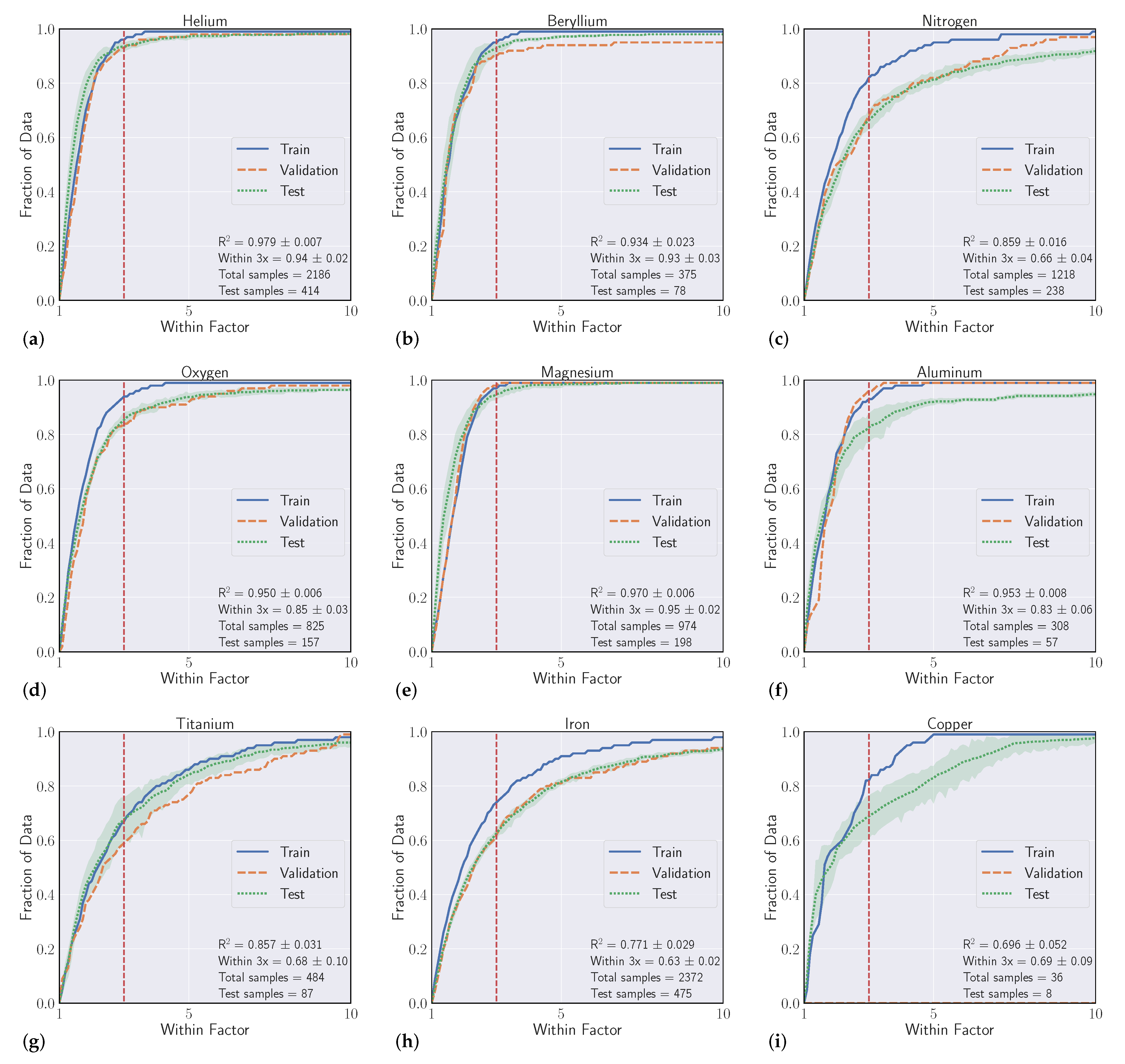
We conduct a series of experiments to show the efficacy of using machine learning models to regress Einstein A-coefficients directly from spectroscopic transition data. The first set of experiments are labeled as ’intraelement’ and the second we denote as ’interelement’ models. Intraelement models are single element, meaning the training, validation, and test sets all come from the same element. Interelement models extend a single model to predict coefficients from multiple elements. That is, the training and validation sets are a combination of multiple elements, and the model is tested on single element test sets. We describe the datasets, metrics, and model selection process with more detail in the following section.

3.1. Datasets

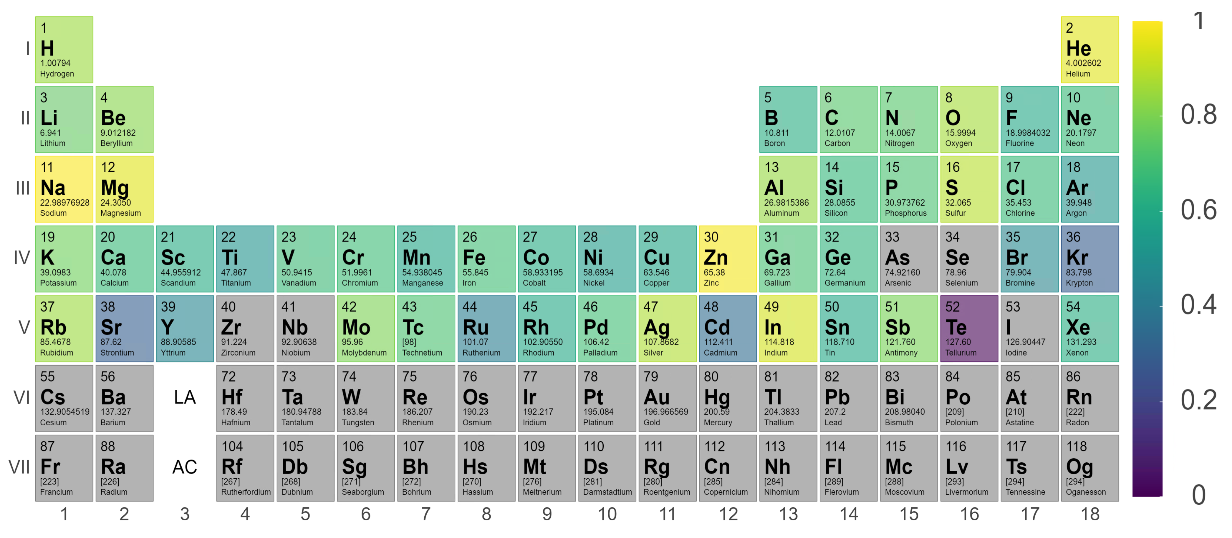
Our experiments were guided by the availability of data within the NIST ASD, where transitions from elements with atomic number Z > 50 quickly become sparse. We curated datasets from the first five rows of the periodic table, excluding arsenic (Z = 33), selenium (Z = 34), zirconium (Z = 40), niobium (Z = 41), and iodine (Z = 53) solely based on data availability. With a large set of spectroscopic transitions spanning nearly 50 elements, we intended to compile interesting findings and correlations that could help inform when models are high and low performing.
More concretely, let E be the set of 49 elements we were able to acquire data from and can be seen in Table A1. For E E , intraelement experiments are based on a data matrix X E n × p and vector y E for a single element ( | E | = 1 ) described by the encoding scheme in Section 2. n is defined as the number of transitions with published A-coefficients and let p be the number of features describing each spectroscopic transition of E. We randomly subset { X E , y E } into train (70%), validation (10%), and test (20%) sets and train a variety of models for the regression task. The training set is the data used to fit the model, the validation set is the data used to evaluate the parameters found during training, and the test set is the data held out to evaluate the model performance on never before seen data.

3.2. Metrics

Our goal in these experiments is to find a regressive function f E : p 
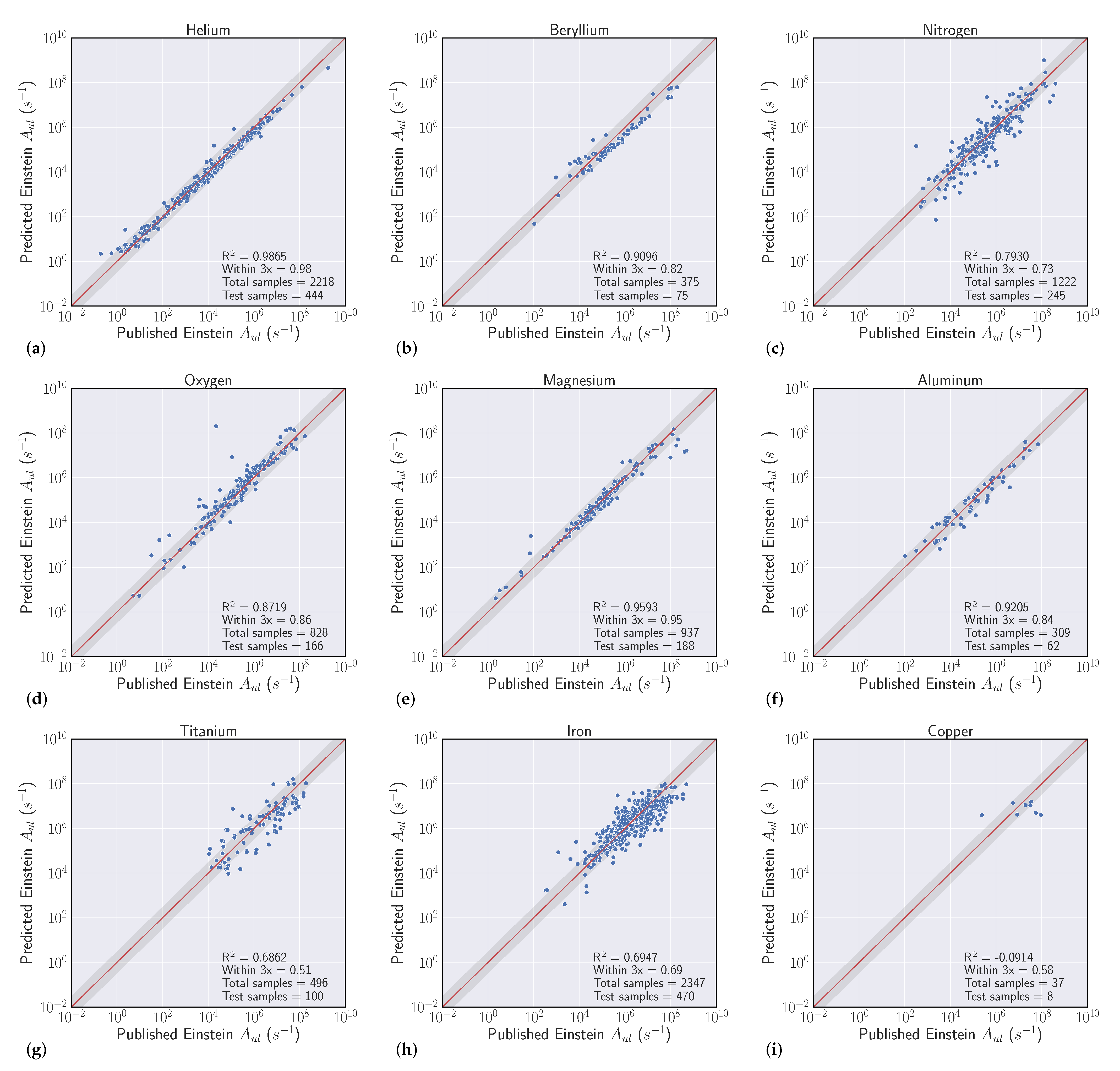
which achieves the best fit to a held out validation set which generalizes to unforeseen data (the test set). We evaluated model fit with two separate scores. The first is to use the typical R 2 metric for regression, which is the square of the Pearson correlation coefficient between predicted y ^ E and actual y E A-coefficients (note that y i E + ). Even though we optimize our models to reduce Mean Squared Error (MSE) [34], where R 2 
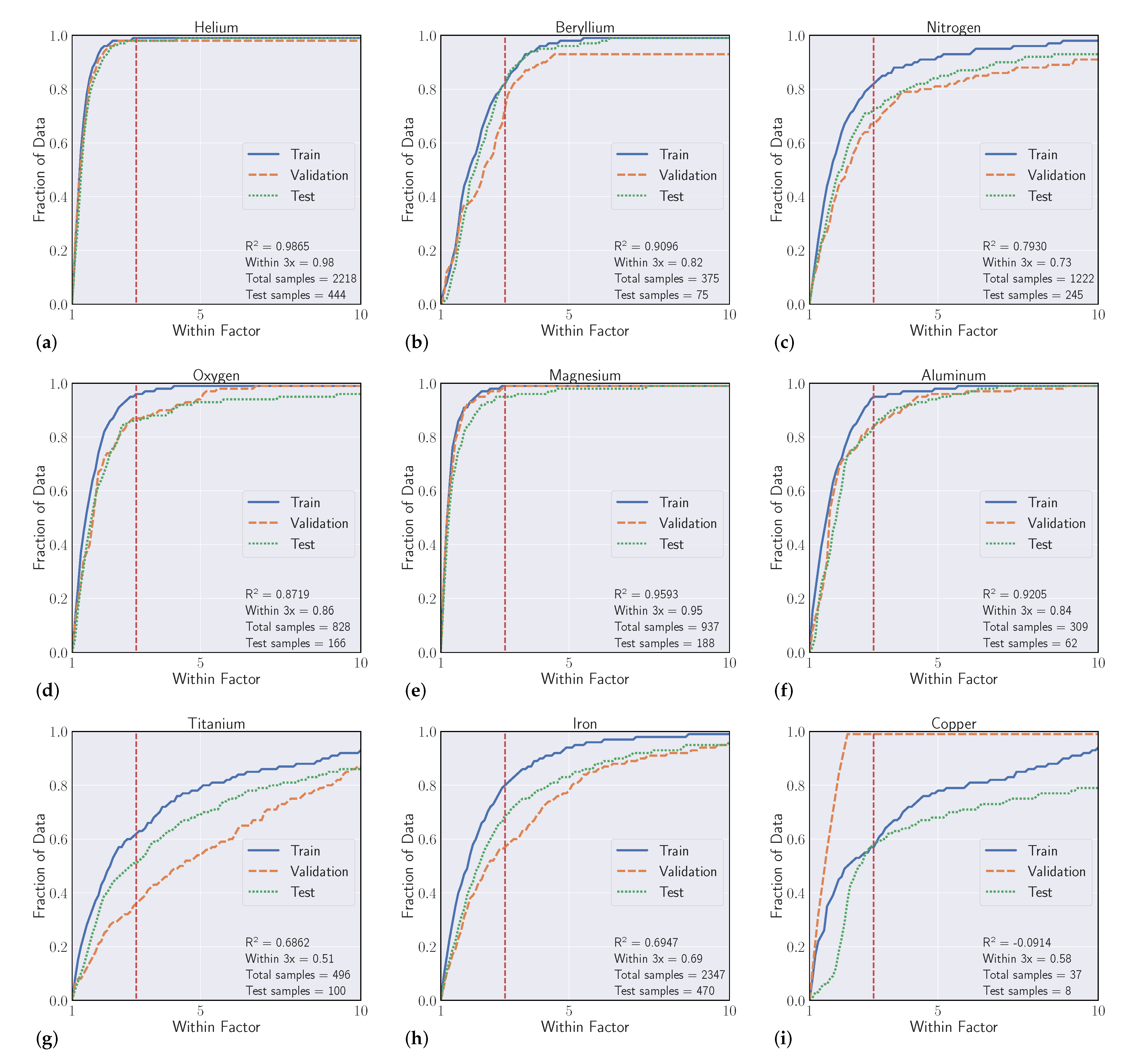
is a standard metric, the second score is more relevant to our particular task, which we refer to as the ’within-3x’ score. Within-3x, or W 3 X ( · , · ) refers to the percentage of predicted transitions that fall within a factor of three of the predicted value and is defined by Equation (1), where 1 is the indicator function and D 
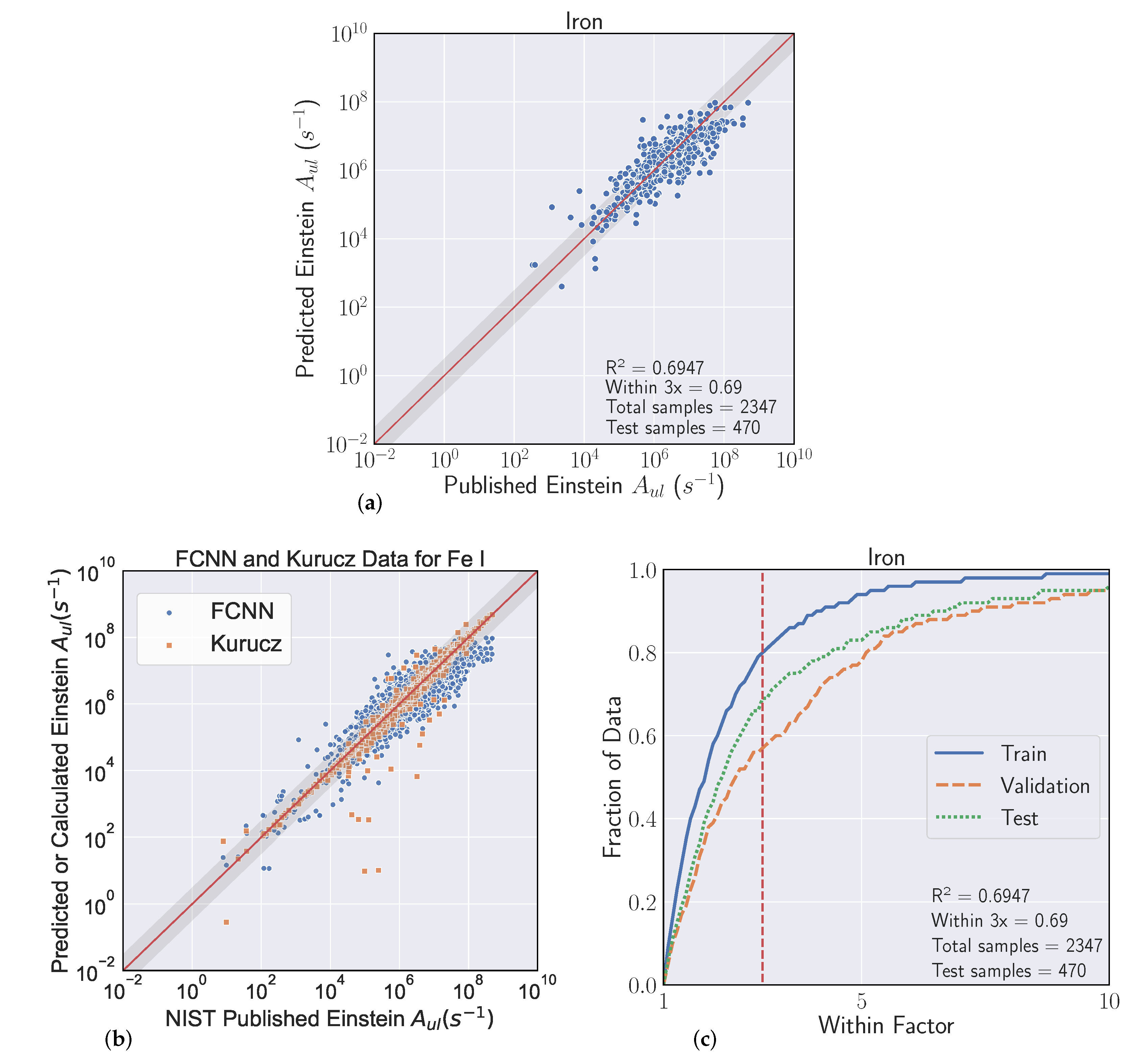
is the indices of the data set. The within-3x score was used in previous work [9] when comparing experimental data to the published values in the Kurucz Atomic Spectral Line Database [10].
W 3 X ( y E , y ^ E ) = 1 | D | i D 1 1 3 < y i ^ y i < 3
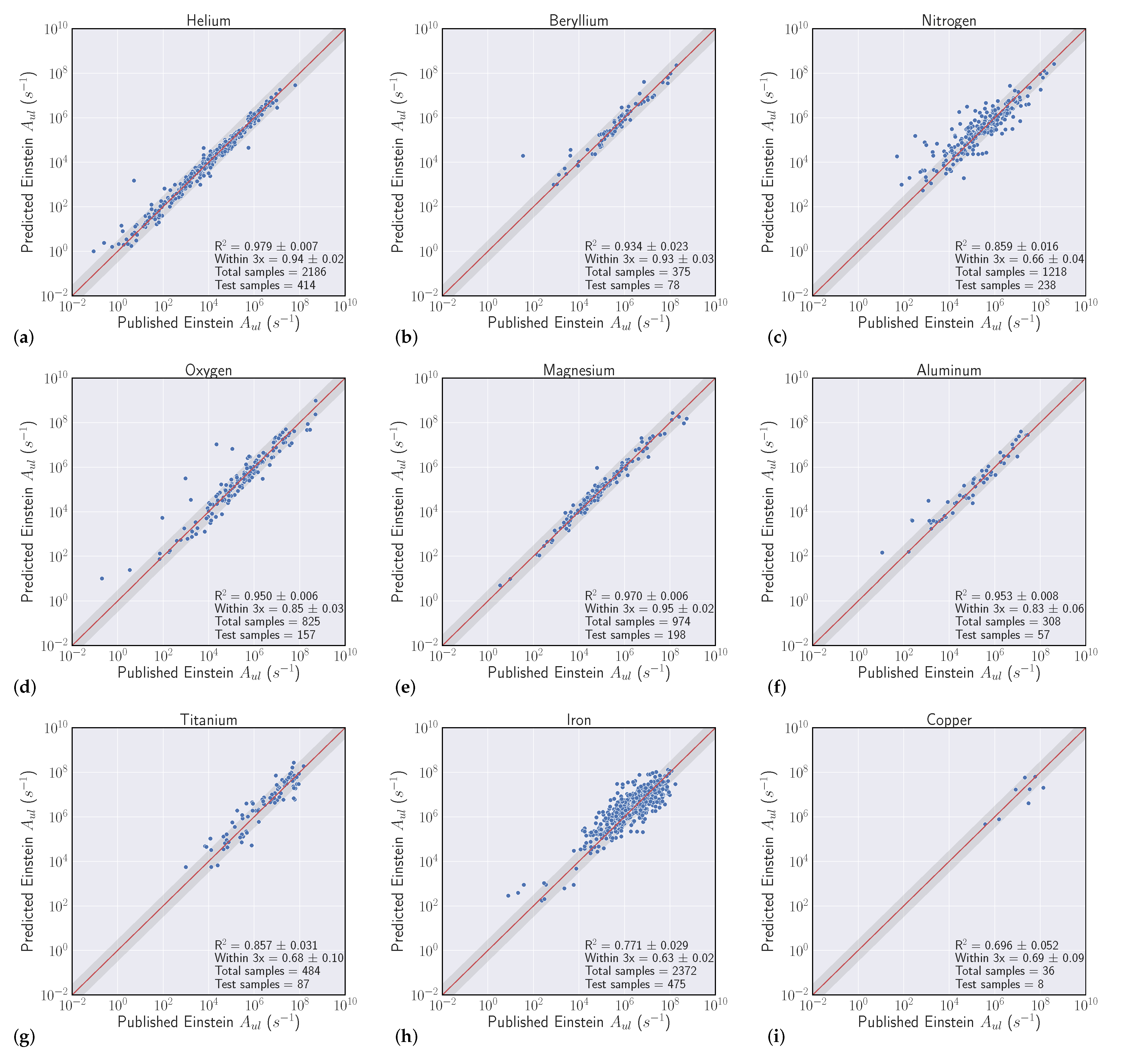
Interelement experiments are similarly constructed to intraelement models. The major difference being that the set of elements chosen for a particular dataset is greater than one | E | > 1 . In this experimental setup, we experience the case where the length of features differs as a function of element p E i p E j i , j D . To mitigate, we constrain all data to include the largest common subset of features between all elements of E.

3.3. Model Selection

Our model search spanned the typical set of supervised regression methods found in most machine learning textbooks [34,37]. Namely, linear methods for regression such as least squares, ridge regression, and lasso regression, tree methods such as random forests, support vector machines, and nonlinear fully connected neural networks (FCNN). During an initial method selection phase, we evaluated these separate methods on a small set of intraelement datasets. Our model evaluation showed that FCNNs with rectified linear unit activation functions consistently outperformed the other models in W 3 X and R 2 regardless of feature engineering for nearly every element tested. After this initial candidate model phase, we used extensive hyperparameter optimization over the FCNN architectures, permuting the number of neurons, layers, epochs, batch sizes, optimizers, and dropout. We randomly sample 1000 model configurations for each intra- and interelement model and optimize each FCNN to minimize a MSE loss function with respect to the training set using gradient descent based methods. Each model is evaluated against the validation set using MSE and the lowest error model is selected as our optimal model. Most of the selected model architectures are 3–5 layers deep with 50 hidden units in each layer. Because the models architectures are relatively small (low memory usage), fast to train (less than 2 min), and are constrained to FCNNs, we argue that there is room to improve model performance with additional architecture complexity.

4. Results and Discussion

We experimentally validated our proposed framework using data from the first five rows of the periodic table in the section below. We begin with intraelement modeling and directly compare our results with published theoretical Hartree–Fock calculations for iron. We then discuss how we can augment model performance for poor performing elements using interelement models. Lastly, we examine which features of our data translate into high and low performance of our models for the purposes of informing future modeling and improved data encoding schemes.

4.1. Intraelement Model Performance

As described in Section 3, intraelement experiments are defined by a single model whose data come from a single element. Our hypothesis was that, with a vast collection of data, we would be able to potentially isolate elemental characteristics that translate into high/low performance. One method to gain a comprehensive view of the FCNN predictions for all the modeled elements is to visualize model performance as a function of color displayed on the periodic table. Figure 1 and Figure 2 display R 2 and W 3 X colored on the periodic table, respectively. Currently, NN models are constructed for each element in the first five periods of the table; however, some element models (shown in gray) are discarded from analysis due to a lack of tabulated transition probabilities in NIST with the given query parameters, such as selenium. Figure 1 portrays a zero R 2 value for some models (shown in purple); generally, intraelement models with small datasets, such as copper, have only a few transition probability values closely grouped. A small deviation from the y ^ e = y e line within this grouping easily introduces a model with a negative R 2 metric which is clipped at zero for enhanced contrast. To better judge overall performance, it is preferred to assess the combination of R 2 and W 3 X .
A subset of elements that have poor R 2 scores in Figure 1 rank relatively high when looking at W 3 X scores of Figure 2. For example, copper has 58% of its tested transition probabilities within a factor of three of the published values even though its R 2 metric is negative. Alternatively, tellurium models score relatively poorly on both R 2 and W 3 X . Overall, we see a trend that, when models perform relatively high, the R 2 and W 3 X agree with each other, but poor performing models require another angle to show the more complete picture.
Figure 2 indicates that 26% of the elements have models with greater than 80% of their predicted transition probabilities within a factor of three relative to published values. Figure 1 and Figure 2 also indicate that performance tends to decrease for both metrics as the period increases. The first three periods appear to have improved performance relative to periods four and five, with period five having the worst performance when both metrics are considered. In addition, the S-block elements generally have higher performance than other element blocks in the table. This is likely due to the reduced complexity in electron configurations for S-block elements, as well as a lack of tabulated transition probabilities of higher Z elements relative to the S-block elements.
We apply a finer grained analysis by examining individual predicted transition probabilities from the testing data set compared against actual published values from the NIST ASD, as demonstrated for iron in Figure 3a. Each point in the scatter plot represents a single predicted transition. The solid red line represents a perfect predicted transition probability value relative to the published NIST value and the shaded region represents the within-3x region. In the example of iron, data are homoskedastically distributed around the linear regression and the test data for this element is grouped primarily between transition probabilities of 10 4 and 10 8 . Note in Section 3 that the within-3x region is applied in previous work [9] when comparing experimental data to the published values in the Kurucz Atomic Spectral Line Database [10].
Figure 3b shows such a comparison between the full dataset (training, validation, and testing) of neural network predictions for neutral iron and the Kurucz neutral iron atomic dataset. The transition probabilities predicted by the neural network relative to the NIST published values are plotted in comparison to the Kurucz calculated transition probabilities relative to the NIST published values. The Kurucz and NIST datasets share some sources for their values and, therefore, have nearly perfect agreement for a subset of transition probabilities. The spread of neural network predictions is seen to be grouped well around the Kurucz dataset. Quantitatively, 69% of the predicted testing values lie within a factor of three of the NIST values while 94% lie within a factor of three for the Kurucz dataset. The fraction of predictions within this 3x space is explicitly shown in Figure 3c for the iron neural network dataset. The chart shows the fraction of predicted values within a factor of the actual published value for the training, validation, and testing data subsets for iron. A factor of one represents a perfect prediction. The vertical dashed line indicates the factor of three represented by the shaded region in Figure 3a,b as a reference. The R 2 metric and within-3x score are applied to each independent elemental model as a method for performance comparisons.
Nine intraelement models from across the periodic table are sampled to provide a more comprehensive view of the actual vs. predicted performance metric of FCNN intraelement models. Shown in Figure 4 are plots of the predicted Einstein A-coefficients against the Einstein A-coefficients published in the NIST ASD for these nine elements. It is evident from Figure 4 that elements such as helium and iron contain more samples for training and testing than elements such as beryllium and titanium. This is merely a function of the number of available tabulated transition probabilities for these elements in the NIST ASD. However, elements that contain many tabulated transitions across a wide dynamic range of transition probability magnitudes, such as helium and magnesium, tend to generate models that predict probabilities more accurately. Some models such as iron have many available transitions in the training set but many of the values only span a limited range of transition probability values. The limited dynamic range of transition probabilities that these models have available for training tends to lead to predictions that have more spread in their prediction distributions. This effect is observed in the relatively lower performing model outputs for iron, nitrogen, and titanium.
The training, validation, and testing performance is more quantitatively assessed in Figure 5 which displays the fraction of predicted transition probability values within a factor of the published value for the same nine intraelement models. A factor of one indicates that fraction of data are perfectly predicted while the vertical dashed line in the individual plots, again, indicates the factor of three threshold for which the broader metric is calculated. The best performing models, such as helium and magnesium, all have a high fraction of predicted values below the 3x threshold. In addition, the performance of the training, validation, and test sets for these models do not readily deviate from one another. The intraelement models with lower performance tend to have training sets that perform well but show lower performance on the testing set. The full set of tabulated performance metrics and performance plots for each element can be found in Appendix A.

4.2. Interelement Model Performance

Subsequent to assessing performance of the intraelement models, the next obvious approach is to determine if training a FCNN model on multiple elements rather than a single element improves prediction performance. In this method, an interelement model is trained using the transitions from across the nine elements previously discussed in Section 4.1. The dataset is constructed such that it encompasses the largest common subset of features between the nine elements (see Section 3). Upon testing, the interelement model is tested on a single element to assess its performance relative to the intraelement model. The prediction performance of the interelement model for the R 2 and fraction of predictions within 3x are plotted in Figure 6 and Figure 7 and the metrics are quantitatively summarized in Table 3. A 95% confidence interval band is shown for the top 5 models found during hyperparameter search over the test set in Figure 7. Similarly, sample mean and standard deviation of R 2 and W 3 X for the top 5 models is given in Table 3.
The data in Table 3 indicate that the interelement model does enable improved prediction performance in the majority of cases. When comparing the R 2 values for predicted vs published regressions, intraelement models that already had reasonably good performance did not significantly benefit from training on additional transitions from other elements. In some cases, the performance of these models is slightly decreased, as is the case for beryllium, helium, and aluminum. However, for intraelement models that perform poorly such as copper, titanium, and iron, the interelement model significantly improved prediction performance.
In a dramatic case, the titanium R 2 and within-3x scores are improved from 0.68 to 0.85 and 51% to 68%, respectively, and can be qualitatively seen by comparing Figure 4 and Figure 6. Likewise, a similar trend is observed for copper model. Of the nine elements used for interelement model training and testing, eight of the elements showed improved R 2 metrics while six showed improved or approximately unchanged within-3x score. This improvement in testing performance indicates that information from transitions of one element can inform the model prediction of transition probabilities for other elements. For example, a trend we see is that modeling can be improved by using additional training data across a wider dynamic range of transition probabilities over multiple elements rather than just a single element being trained on.

4.3. Element Model Feature Importance

An inherent challenge with using a machine learning approach to predict transition probabilities is the explainability of the model. Shapley values can potentially provide insight into what features are most significant to the FCNN model, as they estimate feature importance by describing the marginal contribution of a single feature to each transition separately. Recent studies have suggested issues with implementing Shapley values for feature importance measures [39], but the technique is a common tool in the literature, implemented here to attempt to provide insight into our transition probability predictions models.
SHAP (Shapley Additive Explanations), a framework developed by Lundberg and Lee, defines a kernel-based additive feature attribution method for estimating Shapley values using a linear explanation function [40]. As the Shapley values for our transition probability models are prohibitively computationally expensive to solve for, this approach is used to estimate the Shapley values for each transition. For each intraelement model, the linear explanation function is found using a background of up to 100 samples from the training set. The feature importance values for an element are estimated using the mean magnitude of the Shapley values for that feature across all transitions in the test set. In particular, the SHAP values for each transition were taken as the coefficients of the linear explanation function:
g ( z ) = ϕ 0 + i = 1 M ϕ i z i
where ϕ j is the effect of feature j, and z { 0 , 1 } M is a coalition of features where M is the size of the largest coalition. This linear function was found by optimization using the SHAP kernel across a sample of the set of all possible coalitions.
In general, trends in the Shapley value analysis suggest that both models and individual predictions which depend heavily upon the Ritz Wavelength tend to perform far worse than ones which heavily depend on orbital configuration terms. We come to this conclusion by comparing two subsets of elements with a relatively large number of available transition probabilities from the NIST ASD: one set of elements with relatively high-performing intraelement models (helium, aluminum, magnesium, nitrogen, and oxygen) and one set of relatively low-performing intraelement models (molybdenum, titanium, vanadium, iron, and chromium).
Quantitatively shown in Figure 8 are the top 20 most important features between each subset. A clear distinction shows that high performing models rely on a different subset of features than the low performing models. From Section 4.1 experiments, we saw that even the worst predictions made by high performing models such as helium and magnesium are reasonable by the standards set by low performing models such as iron. We then asked the question of whether high and low performing predictions within each subset rely on a similar set of features. Figure 9 and Figure 10 show the collective mean Shapley values for the top and bottom 10% of predictions (by absolute error) for the high performing and low performing sets, respectively. To our surprise, we saw the poor performing subset of models, regardless of high and low error predictions (Figure 10), heavily rely on the Ritz Wavelength feature more than any other feature. More notably, the highest error predictions from the high performing models also showed a large reliance on Ritz Wavelength. A finer grained analysis showed that most predictions from the subset of low performing intraelement models heavily rely on the Ritz Wavelength. From the predictive model perspective, it’s difficult to answer why a heavy reliance upon this feature seems to imply poor performance, but, from the atomic spectroscopy viewpoint, it’s an interesting finding. We see a similar finding for non-configuration features such as upper/lower multiplicity and upper/lower energy, but the Shapely strengths are much weaker. Our intention is that these types of finding can further help in developing higher performing predictive models by the community.
Earlier in Section 2, it was assumed that feature representation of spectroscopic transitions would be intimately aligned with nuclear and electronic structural configurations as these are the fundamental parameters informing theoretical calculations. The configuration describes the wavefunction, which subsequently provides the overlap integral for the transition probability. Energy states with a defined configuration provide an opportunity to inform the model during training about the orbital distribution of the electrons in the upper and lower energy states for a given transition. Our analysis suggests the configuration features are indeed some of the most important features to high performing models.

5. Conclusions

As machine learning becomes more prevalent in physical science, it is critical that communities investigate which problem types are amenable to its application and the accuracy machine learning tools offer in these problem spaces. In this investigation, we tested the feasibility of using machine learning and ultimately FCNNs to predict fundamental spectroscopic constants based on the electronic structure of atoms, particularly prediction of transition probabilities. In contrast to analyzing raw spectral data with machine learning, our approach implemented neural networks to predict broadly applicable spectral constants which inform forward models removing the temperature and instrument dependence of spectral information that may otherwise limit the scope of machine learning analysis.
Our results show that NNs are capable of predicting atomic transition probabilities and learning from the feature set of novel electronic orbital encodings we developed. The absolute accuracy of the predicted transition probabilities is typically observed to be lower than can be calculated with modern theoretical methods or experiments for elements with lower atomic numbers (see Section 4.1). However, the value proposition of increased speed (a few minutes for training and seconds for inference) and reduced resources to acquire transition probability values via neural network prediction is appealing for many applications based on the accuracy that was achieved.
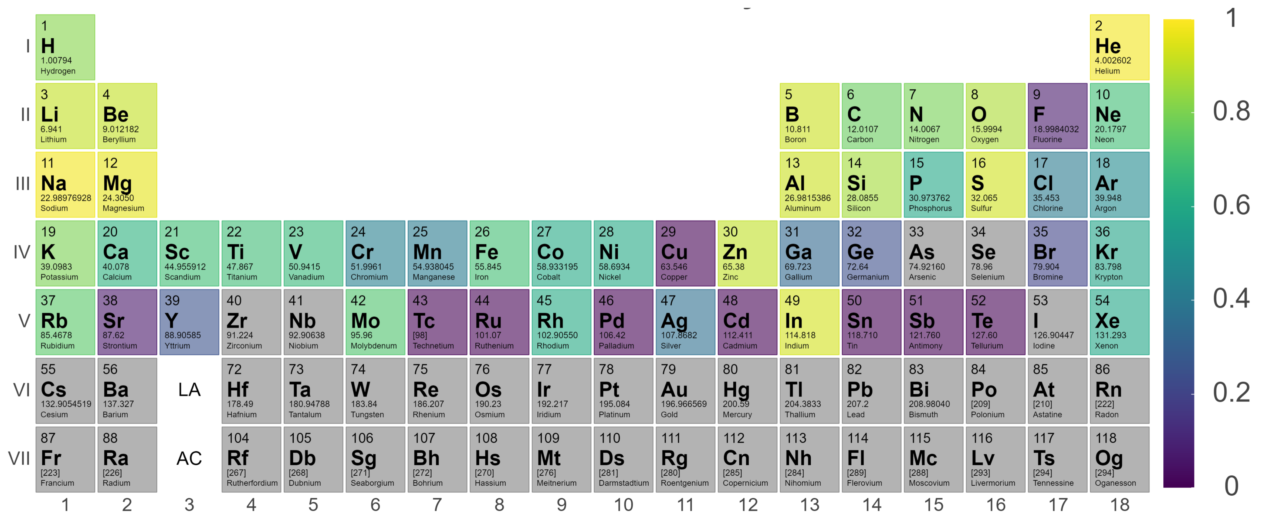
Overall, our experiments showed that S-Block elements are typically higher performing than higher periods of the periodic table. Intuitively, elements that have a small number of atomic transitions perform worse than elements with a larger amount of data. Though this poor performance can typically be augmented with data from other elements to improve overall performance. Additionally, model performance is heavily dependent upon feature representation of each atomic transition and we see model performance gains to be had in this space. For example, our 
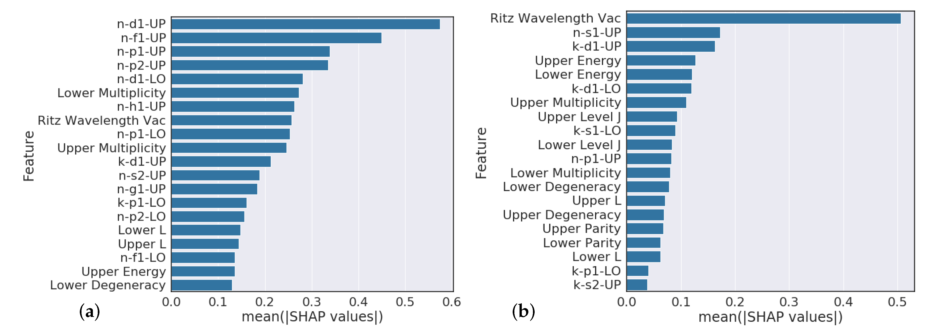
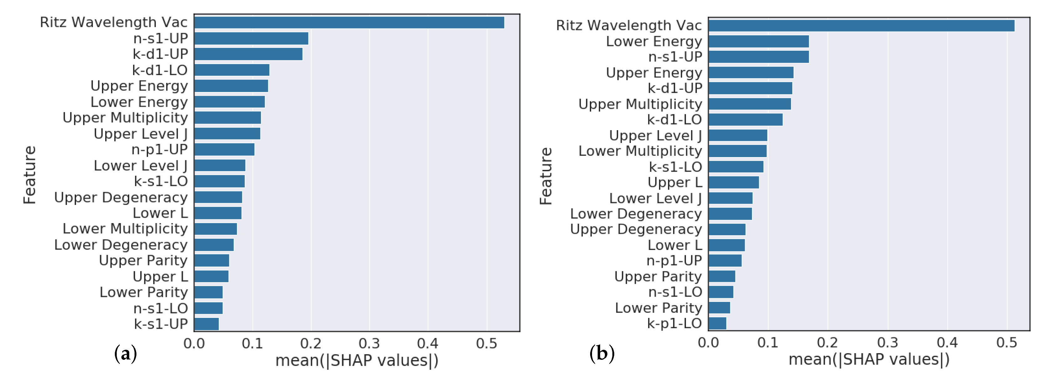
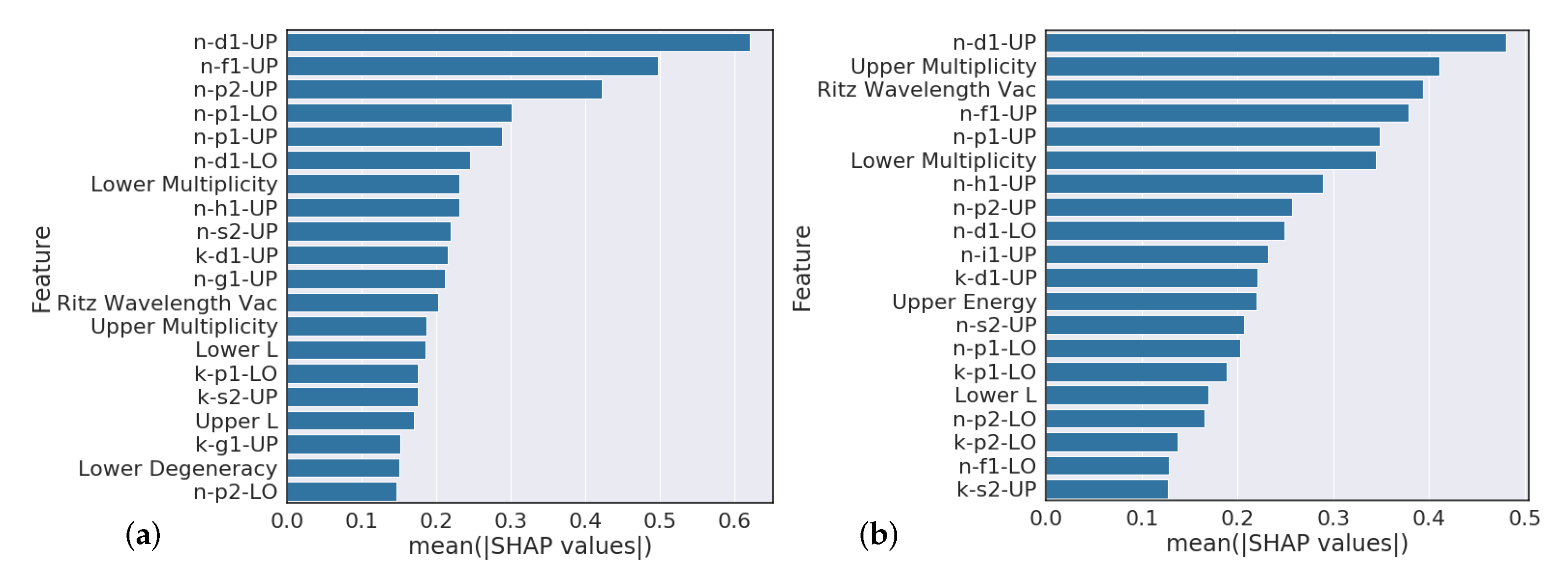
Section 4.3 analysis suggests that model predictions that heavily rely on the Ritz wavelength are indicators of poor performance while models that heavily rely on orbital information are typically higher performing. Further feature engineering to reflect this finding could give modest performance gains.
Significant potential in this technique still remains if the accuracy and dynamic range of neural network predictions are improved on in the future. This technique offers orders of magnitude speed up compared to traditional methods. The technique would allow not only new spectra to be explored, but it would also enable quality checking of previously reported values and allow modeling of transitions that are known, but have not been measured yet. As theoretical transition probability calculations and experimental accuracy are improved over time, the inputs to the machine learning models will also improve, thereby potentially enhancing the value of the NN approach for non-measured or non-calculated transitions.
Our future efforts in this area will focus on improving optimization of neural network models, determining the minimum and most important subsets of features required for accurate predictions, and attempting to extend this technique to higher Z elements on the periodic table as well as ions. Additionally, it is of interest to determine if training on specific periodic table trends (e.g., only transition metals) increases the accuracy for elements in that trend.

Author Contributions

C.M.M., J.D.Z. and M.D.C.; Methodology, All; Software, J.J.M., L.W., A.J.V.O., and J.D.Z.; Validation, All; Formal Analysis, All; Data Curation, All; Writing—Original Draft Preparation, All; Writing—Review and Editing, All; Visualization, J.J.M., L.W., A.J.V.O., and J.D.Z.; Project Administration, M.D.C. All authors have read and agreed to the published version of the manuscript.

Funding

Sandia National Laboratories is a multimission laboratory managed and operated by National Technology Engineering Solutions of Sandia, LLC, a wholly owned subsidiary of Honeywell International Inc., for the U.S. Department of Energy’s National Nuclear Security Administration under contract DE-NA0003525. This paper describes objective technical results and analysis. Any subjective views or opinions that might be expressed in the paper do not necessarily represent the views of the U.S. Department of Energy or the United States Government.

Institutional Review Board Statement

Not applicable.

Informed Consent Statement

Not applicable.

Data Availability Statement

All encoded transitions and transition probability data is available upon request.

Conflicts of Interest

The authors declare no conflict of interest.

Abbreviations

The following abbreviations are used in this manuscript:
ASDAtomic Spectra Database
FCNNFully Connected Neural Network
MLMachine Learning
NISTNational Institute of Standard and Technology
NNNeural Network
SHAPShapley Additive Explanations

Appendix A

For completeness and transparency, the full set of results from all elements used in our experiments is provided below. Included in Table A1 is a collection of quantitative metrics from the intraelement and interelement experiments. This is followed by a complete set of the predicted vs published and ‘within factor’ plots for each intraelement experiment.
Table A1. Performance metrics for all elements investigated.
NameSamplesIntraelement Within 3xIntraelement R2Interelement Within 3xInterelement R2
Aluminum3090.840.92050.83 ± 0.060.953 ± 0.008
Antimony100.79−2.2836NANA
Argon4280.520.4815NANA
Beryllium3750.820.90960.93 ± 0.030.934 ± 0.023
Boron2530.630.9189NANA
Bromine530.470.1994NANA
Cadmium180.35−0.1567NANA
Calcium1360.670.6388NANA
Carbon16020.730.767NANA
Chlorine960.670.405NANA
Chromium5270.680.4334NANA
Cobalt3380.610.602NANA
Copper370.58−0.09140.69 ± 0.090.696 ± 0.052
Fluorine1180.590.0682NANA
Gallium230.70.3369NANA
Germanium260.650.2397NANA
Helium22180.980.98650.94± 0.020.979 ± 0.007
Hydrogen1380.850.8198NANA
Indium270.930.9325NANA
Iron23470.690.69470.63 ± 0.020.771 ± 0.029
Krypton1830.290.5768NANA
Lithium2570.760.9075NANA
Magnesium9370.950.95930.95 ± 0.020.97± 0.006
Manganese4630.580.409NANA
Molybdenum7210.80.7205NANA
Neon5330.670.6891NANA
Nickel4280.550.602NANA
Nitrogen12220.730.7930.66 ± 0.040.859 ± 0.016
Oxygen8280.860.87190.85 ± 0.030.95 ± 0.006
Palladium80.69−1.3638NANA
Phosphorus990.710.5899NANA
Potassium2070.780.7985NANA
Rhodium1110.60.6065NANA
Rubidium400.850.742NANA
Ruthenium110.42−8.4747NANA
Scandium2600.610.688NANA
Silicon5630.660.8615NANA
Silver70.880.3603NANA
Sodium4960.990.9791NANA
Strontium860.30.0599NANA
Sulfur8930.890.9269NANA
Technetium130.71−4.7655NANA
Tellurium60−8.9116NANA
Tin550.59−1.2858NANA
Titanium4960.510.68620.68 ± 0.100.857 ± 0.031
Vandium9930.670.6658NANA
Xenon1870.620.5887NANA
Yttrium1890.450.2527NANA
Zinc160.980.9042NANA
Table A2. Example feature vector representation for the transition of iron I from excited state energy 19,350.891 cm 1 (Configuration: 3d 6 ( 5 D)4s4p( 3 P°), Term Symbol: 7 D°) to ground state (Configuration: 3d 6 4s 2 , Term Symbol: 5 D).
Feature NameEncoded Value
Ritz Wavelength Vaclog(516.77207 + 1)
Accuracy3
n-s1-LO4
k-s1-LO2
n-s2-LO0
k-s2-LO0
n-p1-LO0
k-p1-LO0
n-p2-LO0
k-p2-LO0
n-d1-LO3
k-d1-LO6
n-d2-LO0
k-d2-LO0
n-s1-UP4
k-s1-UP1
n-s2-UP0
k-s2-UP0
n-p1-UP4
k-p1-UP1
n-p2-UP0
k-p2-UP0
n-d1-UP3
k-d1-UP6
n-d2-UP0
k-d2-UP0
Lower Level J4
Upper Level J5
Lower Energylog(0 + 1)
Upper Energylog(19,350.891 + 1)
Lower Multiplicity2
Upper Multiplicity3
Lower L2
Upper L2
Lower Parity−1
Upper Parity1
Lower Degeneracy9
Upper Degeneracy11
Akilog(1450 + 1)
Period4
Group8
Atomic Number26
Atomic Mass55.845
Protons26
Neutrons30
Electrons26
LS-LO1
JJ-LO−1
JL-LO−1
LS-UP1
JJ-UP−1
JL-UP−1
Atoms 09 00002 i001
Atoms 09 00002 i002
Atoms 09 00002 i003
Atoms 09 00002 i004

References

  1. Hanson, R.K.; Spearrin, R.M.; Goldenstein, C.S. Spectroscopy and Optical Diagnostics for Gases; Springer: Berlin/Heidelberg, Germany, 2016; Volume 1. [Google Scholar]
  2. Laurendeau, N.M. Statistical Thermodynamics: Fundamentals and Applications; Cambridge University Press: Cambridge, UK, 2005. [Google Scholar]
  3. Träbert, E. Critical assessment of theoretical calculations of atomic structure and transition probabilities: An experimenter’s view. Atoms 2014, 2, 15–85. [Google Scholar] [CrossRef] [Green Version]
  4. Kramida, A. Critical evaluation of data on atomic energy levels, wavelengths, and transition probabilities. Fusion Sci. Technol. 2013, 63, 313–323. [Google Scholar] [CrossRef]
  5. Wiese, W.L. The critical assessment of atomic oscillator strengths. Phys. Scr. 1996, 1996, 188. [Google Scholar] [CrossRef]
  6. Baker, J. Transition Probabilities for One Electron Atoms; NIST Technical Note 1618; National Institute of Standards and Technology: Gaithersburg, MD, USA, 2008.
  7. Drake, G.W.F. High precision calculations for helium. In Atomic, Molecular, and Optical Physics Handbook; Springer: New York, NY, USA, 1996; pp. 154–171. [Google Scholar]
  8. Wiese, W.L.; Fuhr, J.R. Accurate atomic transition probabilities for hydrogen, helium, and lithium. J. Phys. Chem. Ref. Data 2009, 38, 565–720. [Google Scholar] [CrossRef] [Green Version]
  9. O’Brian, T.R.; Wickliffe, M.E.; Lawler, J.E.; Whaling, W.; Brault, J.W. Lifetimes, transition probabilities, and level energies in Fe I. J. Opt. Soc. Am. B 1991, 8, 1185–1201. [Google Scholar] [CrossRef]
  10. Kurucz, R.L.; Bell, B. Atomic Line Data, CD-ROM, 23, 1995. Available online: https://ui.adsabs.harvard.edu/abs/1995KurCD..23.....K/abstract (accessed on 1 March 2020).
  11. Kurucz, R.L. Semiempirical calculation of gf values, IV: Fe II. SAO Spec. Rep. 1981, 390. Available online: http://adsabs.harvard.edu/pdf/1981SAOSR.390.....K (accessed on 5 January 2021).
  12. Gehren, T.; Butler, K.; Mashonkina, L.; Reetz, J.; Shi, J. Kinetic equilibrium of iron in the atmospheres of cool dwarf stars-I. The solar strong line spectrum. Astron. Astrophys. 2001, 366, 981–1002. [Google Scholar] [CrossRef] [Green Version]
  13. Pehlivan, A.; Nilsson, H.; Hartman, H. Laboratory oscillator strengths of Sc i in the near-infrared region for astrophysical applications. Astron. Astrophys. 2015, 582, A98. [Google Scholar] [CrossRef] [Green Version]
  14. Quinet, P.; Fivet, V.; Palmeri, P.; Engström, L.; Hartman, H.; Lundberg, H.; Nilsson, H. Experimental radiative lifetimes for highly excited states and calculated oscillator strengths for lines of astrophysical interest in singly ionized cobalt (Co II). Mon. Not. R. Astron. Soc. 2016, 462, 3912–3917. [Google Scholar] [CrossRef] [Green Version]
  15. Meggers, W.F.; Corliss, C.H.; Scribner, B.F. Tables of Spectral-Line Intensities: Arranged by Wavelengths; National Institute of Standards and Technology: Gaithersburg, MD, USA, 1974; Volume 145.
  16. Cowley, C.R.; Corliss, C.H. Moderately accurate oscillator strengths from NBS intensities–II. Mon. Not. R. Astron. Soc. 1983, 203, 651–659. [Google Scholar] [CrossRef] [Green Version]
  17. Henrion, G.; Fabry, M.; Remy, M. Determination of oscillator strengths for UI and UII lines. J. Quant. Spectrosc. Radiat. Transf. 1987, 37, 477–499. [Google Scholar] [CrossRef]
  18. Ouyang, T.; Wang, C.; Yu, Z.; Stach, R.; Mizaikoff, B.; Liedberg, B.; Huang, G.B.; Wang, Q.J. Quantitative analysis of gas phase IR spectra based on extreme learning machine regression model. Sensors 2019, 19, 5535. [Google Scholar] [CrossRef] [PubMed] [Green Version]
  19. Chatzidakis, M.; Botton, G.A. Towards calibration-invariant spectroscopy using deep learning. Sci. Rep. 2019, 9, 1–10. [Google Scholar] [CrossRef] [PubMed]
  20. Ghosh, K.; Stuke, A.; Todorović, M.; Jørgensen, P.B.; Schmidt, M.N.; Vehtari, A.; Rinke, P. Deep learning spectroscopy: Neural networks for molecular excitation spectra. Adv. Sci. 2019, 6, 1801367. [Google Scholar] [CrossRef]
  21. Sun, C.; Tian, Y.; Gao, L.; Niu, Y.; Zhang, T.; Li, H.; Zhang, Y.; Yue, Z.; Delepine-Gilon, N.; Yu, J. Machine learning allows calibration models to predict trace element concentration in soils with generalized LIBS Spectra. Sci. Rep. 2019, 9, 1–18. [Google Scholar] [CrossRef]
  22. Liu, J.; Osadchy, M.; Ashton, L.; Foster, M.; Solomon, C.J.; Gibson, S.J. Deep convolutional neural networks for Raman spectrum recognition: A unified solution. Analyst 2017, 142, 4067–4074. [Google Scholar] [CrossRef] [Green Version]
  23. Stein, H.S.; Guevarra, D.; Newhouse, P.F.; Soedarmadji, E.; Gregoire, J.M. Machine learning of optical properties of materials–predicting spectra from images and images from spectra. Chem. Sci. 2019, 10, 47–55. [Google Scholar] [CrossRef] [Green Version]
  24. Lansford, J.L.; Vlachos, D.G. Infrared spectroscopy data-and physics-driven machine learning for characterizing surface microstructure of complex materials. Nat. Commun. 2020, 11, 1–12. [Google Scholar] [CrossRef]
  25. Kramida, A.; Ralchenko, Y.; Reader, J.; NIST ASD Team. NIST Atomic Spectra Database (ver. 5.7.1) [Online]; National Institute of Standards and Technology: Gaithersburg, MD, USA, 2019. Available online: https://physics.nist.gov/asd (accessed on 1 May 2020).
  26. Khalid, S.; Khalil, T.; Nasreen, S. A Survey of Feature Selection and Feature Extraction Techniques in Machine Learning. In Proceedings of the 2014 Science and Information Conference, London, UK, 27–29 August 2014; pp. 372–378. [Google Scholar]
  27. Kearnes, S.; McCloskey, K.; Berndl, M.; Pande, V.; Riley, P. Molecular graph convolutions: Moving beyond fingerprints. J. Comput. Aided Mol. Des. 2016, 30, 595–608. [Google Scholar] [CrossRef] [Green Version]
  28. Behler, J.; Parrinello, M. Generalized neural-network representation of high-dimensional potential-energy surfaces. Phys. Rev. Lett. 2007, 98, 146401. [Google Scholar] [CrossRef]
  29. Willatt, M.J.; Musil, F.; Ceriotti, M. Atom-density representations for machine learning. J. Chem. Phys. 2019, 150, 154110. [Google Scholar] [CrossRef] [PubMed] [Green Version]
  30. Motoda, H.; Liu, H. Feature Selection, Extraction, and Construction; Communication of IICM (Institute of Information and Computing Machinery): Taipei, Taiwan, 2002; pp. 67–72. [Google Scholar]
  31. Ladha, L.; Deepa, T. Feature Selection Methods and Algorithms. Int. J. Comput. Sci. Eng. (IJCSE) 2011, 3, 1787–1797. [Google Scholar]
  32. Froese Fischer, C. The Hartree–Fock Method for Atoms: A Numerical Approach; Wiley: Hoboken, NJ, USA, 1977. [Google Scholar]
  33. Martin, W.C.; Wiese, W. Atomic Spectroscopy: A Compendium of Basic Ideas, Notation, Data, and Formulas; National Institute of Standards and Technology: Gaithersburg, MD, USA, 1999.
  34. Hastie, T.; Tibshirani, R.; Friedman, J. The Elements of Statistical Learning: Data Mining, Inference, and Prediction; Springer: New York, NY, USA, 2009. [Google Scholar]
  35. Martin, W.; Wiese, W. Spectral Lines: Selection Rules, Intensities, Transition Probabilities, Values, and Line Strengths. 2017. Available online: https://www.nist.gov/pml/atomic-spectroscopy-compendium-basic-ideas-notation-data-and-formulas/atomic-spectroscopy (accessed on 1 May 2020).
  36. Kramida, A. Assessing uncertainties of theoretical atomic transition probabilities with Monte Carlo random trials. Atoms 2014, 2, 86–122. [Google Scholar] [CrossRef] [Green Version]
  37. Bishop, C.M. Pattern Recognition and Machine Learning; Springer: Berlin/Heidelberg, Germany, 2006. [Google Scholar]
  38. Cowan, R.D. The Theory of Atomic Structure and Spectra; Number 3; University of California Press: Berkeley, CA, USA, 1981. [Google Scholar]
  39. Kumar, I.E.; Venkatasubramanian, S.; Scheidegger, C.; Friedler, S. Problems with Shapley-value-based explanations as feature importance measures. arXiv 2020, arXiv:2002.11097. [Google Scholar]
  40. Lundberg, S.M.; Lee, S.I. A unified approach to interpreting model predictions. In Advances in Neural Information Processing Systems; pp. 4765–4774. Available online: https://papers.nips.cc/paper/2017/hash/8a20a8621978632d76c43dfd28b67767-Abstract.html (accessed on 5 January 2021).
Figure 1. R 2 metric applied to modeled elements across the first five periods of the periodic table.
Atoms 09 00002 g001
Figure 2. W 3 X applied to modeled elements across the first five periods of the periodic table.
Atoms 09 00002 g002
Figure 3. Performance metrics for iron neural network predictions. (a) comparison of predicted vs. published NIST transition probability test set; (b) comparison with Kurucz atomic data for Fe I electric dipole transitions showing spread between FCNN predictions and the Kurucz data relative to the published NIST values; (c) fraction of predicted values within a factor of the published transition probability value for the training, validation, and test sets.
Atoms 09 00002 g003
Figure 4. Predicted vs. published Einstein A-coefficients for intraelement models.
Atoms 09 00002 g004
Figure 5. Performance of intraelement models showing fraction of transition probability predictions within a factor of the published value for training, validation, and testing sets.
Atoms 09 00002 g005
Figure 6. Predicted vs. published Einstein A-coefficients for the interelement model.
Atoms 09 00002 g006
Figure 7. Performance of interelement models showing fraction of transition probability predictions within a factor of the published value for training, validation, and testing sets.
Atoms 09 00002 g007
Figure 8. SHAP feature importance results. (a) high performing models (helium, aluminum, magnesium, nitrogen, and oxygen); (b) low performing models (molybdenum, titanium, vanadium, iron, and chromium). The configuration parameter labels are in the format {n,k}-L#-{UP,LO}, where n and k denote if the feature is principle quantum number (n) or occupation number (k), L is the orbital angular momentum with the indexed (#) occurrence in the total configuration, and UP/LO associates it with the upper or lower energy level in a transition.
Atoms 09 00002 g008
Figure 9. SHAP feature importance results for subsets of transitions for high-performing models (helium, aluminum, magnesium, nitrogen, and oxygen) (a) Top 10% of transition predictions; (b) Bottom 10% of transition predictions. The configuration parameter labels are in the format {n,k}-L#-{UP,LO} where n and k denote if the feature is principle quantum number (n) or occupation number (k), L is the orbital angular momentum with the indexed (#) occurrence in the total configuration, and UP/LO associates it with the upper or lower energy level in a transition.
Atoms 09 00002 g009
Figure 10. SHAP feature importance results for subsets of transitions for low-performing models (molybdenum, titanium, vanadium, iron, and chromium) (a) Top 10% of transition predictions; (b) Bottom 10% of transition predictions. The configuration parameter labels are in the format {n,k}-L#-{UP,LO}, where n and k denote if the feature is principle quantum number (n) or occupation number (k), L is the orbital angular momentum with the indexed (#) occurrence in the total configuration, and UP/LO associates it with the upper or lower energy level in a transition.
Atoms 09 00002 g010
Table 1. Abbreviated example encoding for the excited electronic configuration of the LS-coupled 19,350.891 cm 1 level of iron I. The subshell of the level is encoded through the column number in the array. The property n represents the principal quantum number and the property k represents the occupancy of the subshell in the nl k nomenclature.
Electron Configuration 3d 6 ( 5 D)4s4p( 3 P°)
Subshells 1 s 2 p 1 p 2 d 1 d 2
Propertynknknknknknk
Encoding410041003600
Table 2. Examples of numerical representation for term symbol in each distinguishable NIST coupling notation. Each coupling type is numerically encoded with a unique one-hot scheme. QN 1 and QN 2 represent the two respective quantum numbers that couple to give J.
Term SymbolCoupling SchemeCoupling EncodingQN 1QN 2Parity
2 P L S    1    −1    −1  0.51−1
(2, 3/2)° J 1 J 2   −1     1    −1  21.51
2 [ 9 / 2 ] ° J 1 L 2 ( K ) or L S 1 ( K )   −1    −1     1  0.54.51
Table 3. Quantitative performance metrics for intraelement and interelement models.
NameSamplesIntraelement within 3xIntraelement R2Interelement within 3xInterelement R2
Aluminum3090.840.92050.83 ± 0.060.953 ± 0.008
Beryllium3750.820.90960.93 ± 0.030.934 ± 0.023
Copper370.58−0.09140.69 ± 0.090.696 ± 0.052
Helium22180.980.98650.94 ± 0.020.979 ± 0.007
Iron23470.690.69470.63 ± 0.020.771 ± 0.029
Magnesium9370.950.95930.95 ± 0.020.970 ± 0.006
Nitrogen12220.730.7930.66 ± 0.040.859 ± 0.016
Oxygen8280.860.87190.85 ± 0.030.950 ± 0.006
Titanium4960.510.68620.68 ± 0.100.857 ± 0.031
Publisher’s Note: MDPI stays neutral with regard to jurisdictional claims in published maps and institutional affiliations.

