Article

Fundamental Parameters Related to Selenium Kα and Kβ Emission X-ray Spectra

1
Laboratory of Instrumentation, Biomedical Engineering and Radiation Physics (LIBPhys-UNL), Department of Physics, NOVA School of Science and Technology, NOVA University Lisbon, 2829-516 Caparica, Portugal
2
LIP—Laboratory of Instrumentation and Particle Physics, Av. Prof. Gama Pinto 2, 1649-003 Lisboa, Portugal
3
BioISI—Biosystems & Integrative Sciences Institute, Faculdade de Ciências da Universidade de Lisboa, Campo Grande, C8, 1749-016 Lisboa, Portugal
4
Laboratoire Kastler Brossel, Sorbonne Université, CNRS, ENS-PSL Research University, Collège de France, Case 74, 4, place Jussieu, F-75005 Paris, France
*
Author to whom correspondence should be addressed.
Submission received: 13 December 2020 / Revised: 12 January 2021 / Accepted: 14 January 2021 / Published: 22 January 2021

Abstract

:
We present relativistic ab initio calculations of fundamental parameters for atomic selenium, based on the Multiconfiguration Dirac-Fock method. In detail, fluorescence yields and subshell linewidths, both of K shell, as well as K β to K α intensity ratio are provided, showing overall agreement with previous theoretical calculations and experimental values. Relative intensities were evaluated assuming the same ionization cross-section for the K-shell hole states, leading to a statistical distribution of these initial states. A method for estimating theoretical linewidths of X-ray lines, where the lines are composed by a multiplet of fine-structure levels that are spread in energy, is proposed. This method provides results that are closer to K α 1 , 2 experimental width values than the usual method, although slightly higher discrepancies occur for the K β 1 , 3 lines. This indicates some inaccuracies in the calculation of Auger rates that have a higher contribution for partial linewidths of the subshells involved in the K β 1 , 3 profile. Apart from this, the calculated value of K β to K α intensity ratio, which is less sensitive to Auger rates issues, is in excellent agreement with recommended values.

1. Introduction

The need of data related to the interactions of light with matter is important in the development of research tools in several fields, such as fundamental physics [1], spectroscopy [2], plasma physics [3], and astrophysics [4]. Atomic calculations constitute an important source of information that partially fulfill this need.
Within this framework, the x-ray emission spectrum has long been a subject of interest, not only because it provides information about the atomic structure through the analysis of the characteristic radiation as, for instance, transition energies, but also because the peaks asymmetry reflects the existence of complex atomic processes beyond a simple bound-bound transition. Nowadays, the atomic structure is adequately explained through the relativistic quantum theory of the atom, whereas profile analysis is a test bed of atomic models.
Among the various atomic systems, inner-shell, multiple open-shell systems, and systems with highly excited states, are the most difficult to handle due to technical issues like the growth of needed computation time, convergence failure, and the existence of multiple near-degenerate eigenstates. Selenium is an example of such systems.
Experimental K-shell fluorescence yields for several atoms, among which Se is included, have been published by several authors. A compilation of the latest results can be found in Kahoul et al. [5]. In what concerns theoretical results, one still relies on the works of Kostroun et al. [6], and Walters and Bhalla [7]. K β / K α intensity ratios have been very recently compiled by Daoudi et al., and although there are a substantial number of experimental data, the theoretical results are scarce.
In the last decade, with the fast development of computational power, emission spectra of open shell systems such as Se, Ti, and Cu could be investigated theoretically. A good way of testing the quality of the calculations is by comparing a synthesized emission spectra with high resolution x-ray data from crystal spectrometers. This has been done by the group of Chantler et al. for Ti [8,9], Cu [10], and V, Sc, Cr, and Mn [9] and by other collaborations bridging together theory and experiment [11,12,13,14,15]. These high resolution spectra might soon be used to update the SRD 128 database [16] run by the National Institute for Standards and Technology, by providing transferable x-ray standards, traceable to the S.I. units, that can be used by the x-ray community to perform high-accuracy calibrations of their systems [17]. Among these recent works are the measurements with a Double-Crystal-Spectrometer (DCS) of Cu [18], Mo [19], and the new microcalorimeter results for the lanthanide metals [20].
In this paper, we report some fundamental parameters related to the x-ray spectra of the selenium isolated atom calculated using the MCDFGME code, developed by Desclaux and Indelicato [21,22], which implements the Multiconfiguration Dirac-Fock code (MCDF) method.

2. Theory

2.1. Atomic Fundamental Parameters

In the context of the MCDF method, an atomic state is characterized by the electronic configuration A, the total angular momentum J, the total magnetic quantum number M, and all other quantum numbers α necessary to fully characterize that state. In the absence of external fields, the energies of these states are degenerate in the total magnetic moment, that is, there are 2 J i + 1 states with identical energies. The set of these degenerate states is called an atomic level, which will then be characterized by ( A , J , α ) . The MCDFGME code developed by Desclaux and Indelicato [23,24] allows for the calculation of the level energies E i as well as radiative R i f , and radiationless R i f N R transition rates between levels i and f. From these quantities one can obtain the other atomic fundamental parameters.
The fluorescence yield of an one-hole atomic configuration A is defined as the probability that a vacancy in the ith subshell is filled through a radiative transition
ω A = i f g i R i f i f g i ( R i f + R i f N R ) ,
where the sum in i is over all the initial levels belonging to the configuration A and the sum in f is over all allowed final atomic levels. The quantity g i = 2 J i + 1 takes into account the degeneracy of the initial level.

2.2. Relativistic Calculations

Level energies and transition probabilities, both radiative and radiationless, were obtained using the multiconfiguration Dirac–Fock method, fully implemented in the general relativistic MCDFGME code developed by Desclaux and Indelicato [23,24].
We will give here a brief description of the MCDF method. For a detailed description we refer the reader to Refs. [23,25,26,27]. The relativistic Hamiltonian is taken in the form
H DCB = a = 1 N h a D + a = 1 N 1 b = a + 1 N V a b CB ,
where h a D is the one-electron Dirac Hamiltonian, and V a b CB describes the sum of Coulomb repulsion and Breit interaction between the ath and the bth electron. Furthermore, the code also accounts for radiative corrections, namely, self-energy and vacuum polarization. For details on Quantum Electrodynamics (QED) corrections, we refer the reader to Ref. [28]. Nuclear size effects were taken into account by using a uniformly charged sphere, and the atomic masses and the nuclear radii were taken from the tables by Audi et al [29], and Angeli [30], respectively.
For the determination of the radiative transition probabilities we followed the formalism proposed by Löwdin [31] to treat the nonorthogonality effects, and consider independently the initial- and final-state wave functions obtained in the so-called optimized level scheme. The length gauge was used for all radiative transition probabilities.
For radiationless transitions, we assumed that the creation of the inner-shell hole is independent of the decay process. The continuum-electron wavefunctions are obtained by solving the Dirac-Fock equations with the same atomic potential of the initial state. To ensure orthogonality in these calculations, no orbital relaxation was allowed between the initial and final bound state wavefunctions.
The code was used in the single-configuration approach, with the Breit interaction and the vacuum polarization terms included in the self-consistent field process, and other QED effects included as perturbations.

2.3. Line Shapes

The width of an atomic level i is given by the sum of all the allowed transition probabilities from this level to all lower-energy levels, both through the emission of a photon (radiative) R i f R and through the emission of an electron (radiationless) R i k N R , multiplied by [32],
Γ i = f R i f R + k R i k N R ,
where the index f represents all one-hole levels that the initial level i can decay to radiatively, and the index k represents all two-hole levels that the level i can decay to via a radiationless emission. The width of a particular transition is connected to its parent- and daughter- level’s lifetimes, thus depending not only on the transition rate from i f , but also on all possible decay pathways that the atom can undergo, both from the initial and the final level. Thus, we can define the width of a given transition to be the sum of the widths of the initial and final levels, as
Γ i f = Γ i + Γ f .
An x-ray “line” is composed, in general, of a multiplet of lines resulting from fine structure levels as shown in Refs. [11,13,32], and thus when trying to compute the line width one has to sum Equation (5) for all of the initial and final levels, i and f, respectively, in the x-ray line manifold,
Γ A B = i f g i Γ i f i g i ,
where the sums run over the initial levels i belonging to the one-hole configuration A and over the final levels f belonging to the one-hole configuration B. This method of computing linewidths is henceforth labeled as “Method 1”.
For example, the transition width of the K α 1 multiplet (in Siegbahn notation) is usually obtained as the sum of the K ( 1 s 1 ) and L 3 ( 2 p 3 / 2 1 ) manifolds (in IUPAC notation), where K represents all of the fine structure levels that arise from a one-hole configuration with a hole in the K shell, while the same is valid for the L 3 subshell.
The K α 1 , 2 and K β 1 , 3 line shapes were obtained, by means of a simulation, from the atomic structure data computed in this work. Similarly to what has been done in previous works (see Refs. [11,13]), the emission line shape (without Doppler broadening) is obtained from the individual transitions between fine structure levels. This is accomplished by summing the contribution of every Lorentzian distribution whose centroid is the transition energy and a natural width given by Equation (4). For comparison with experimental results one has to convolute the simulated line shape with the spectrometer instrumental function in order to get the proper broadening. The intensity of each individual transition is obtained through the expression:
I i f = N i g i g R i f R f R i f R + k R i k N R ,
where N i is a scaling factor that represents the rate of formation of ions in level i per unit volume (in units of s 1 · cm 3 ), assumed here to be equal for all levels. The factor g is the sum of the multiplicities of all the possible levels in the subshell that contains level i. R i f R is the radiative rate of a transition from the one-hole level i to the one-hole level f, while R i k N R corresponds to a radiationless-transition rate between the one-hole level i to the two-hole level k. Once the spectra are synthesized, we can in principle fit it with multiple Lorentzians in a similar fashion to the analysis of experimental spectra to obtain natural linewidths [12,13,33]. If this method is applied to the simulated spectra including only the natural widths of the transitions in a given x-ray line, we will obtain the theoretical natural widths of the lines in question. This will be labeled in this work as “Method 2”. The difference between Method 1 and Method 2 is that in the latter, the influence of the broadening of the line shape due to the energy spread of the multiplet, is already taken into account, whereas in the first method we are just summing the weighted widths of each transition as if all of them had the same energy.
The ratio of the two line intensities belonging to the same initial configuration, such as the K β /K α ratio, depends only on the radiative transition rates, and can be written as:
I A B I A C = i f g i R i f R i f g i R i f R ,
where the sum in f is over all levels belonging to the one-hole configuration B and the sum in f is over all levels belonging to the one-hole configuration C. In Equation (6), the term g i / g represents the probability that a given ion is left in level i after ionization, assuming that all the states are equally probable. This approximation is only valid if the cross sections for the creation of the holes are similar. Note that if we are comparing peaks that originate from the same levels, this factor is the same for both. The second term corresponds to a transition fluorescence yield, that is basically the probability that a radiative transition from level i f occurs taking into account all of the other decay possibilities.
If the simulated spectra were to be compared with experimental results, some broadening mechanisms would have to be included in the simulation. One of the most common ways of including the instrumental broadening or line broadening due to the thermal motion of the atoms that are emitting the x rays (in a gas or plasma), is through the convolution of the natural line shape with a Gaussian profile [34]. This convolution of a Lorentzian and a Gaussian distributions is usually known as a Voigt profile and can be computed by the direct calculation of
V ( E , σ , Γ ) = + G ( E , σ ) L ( E E , Γ ) d E ,
where
G ( E , σ ) = 1 σ 2 π exp ( E E 0 ) 2 2 σ 2 ,
and
L ( E , Γ ) = I i f Γ / 2 π ( E E 0 ) 2 + ( Γ / 2 ) 2 ,
where E is the energy, E 0 is the energy centroid of a particular transition, Γ is the full-width at half-maximum (FWHM) of the Lorentzian profile and σ is the standard deviation of the Gaussian distribution, related to the FWHM α , by α = 2 σ 2 l n 2 . I i , f is the intensity of the transition, given by Equation (6).
Although there is no closed analytical form for the Voigt profile, it can be obtained from the real part of the Faddeeva function, w ( z ) by
V ( E , σ , Γ ) = Re [ w ( z ) ] σ 2 π ,
where z = E + i Γ σ 2 . As with the Fadeeva function, which can be computed from different algorithms [35], there are some other representations of the Voigt function that are usually given in terms of special functions. Some examples are the confluent hypergeometric function [36], the Whittaker function [37], and the Complex Error function [38]. In any simulation, the instrumental broadening can be simulated by the use of Equation (11) or, if the instrumental function is closer to a Lorentzian than to a Gaussian shape as is the case of some crystal spectrometers [11,13], a Lorentzian shape can also be used. This Lorentzian line shape will have a FWHM obtained by summing the natural width to the spectrometer energy resolution, because the convolution of two centered Lorentzian functions is still a Lorentzian function whose width is just the sum of the two. These procedures have been recently applied to compare high-resolution measurements with simulated spectra [12,13,15].

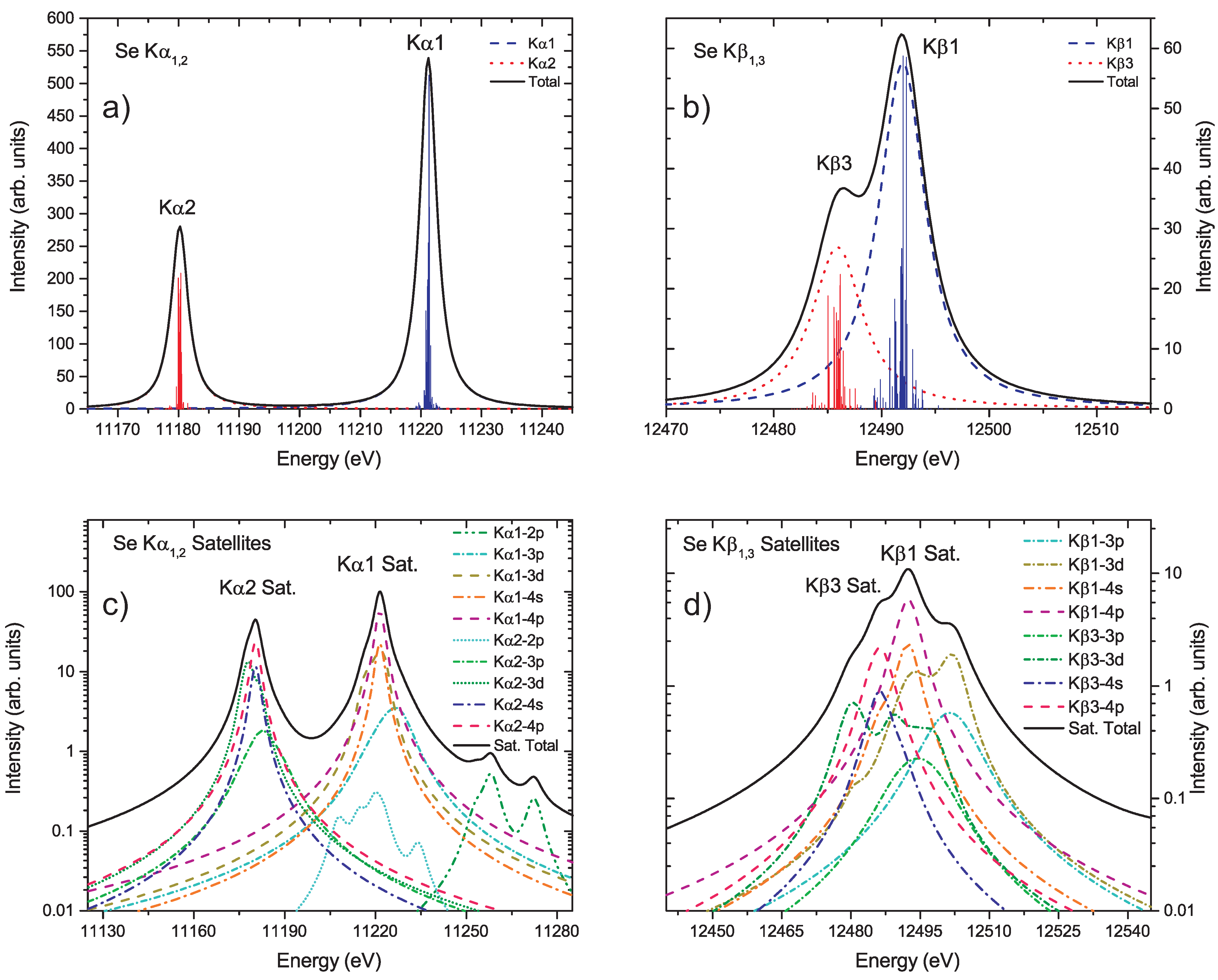
3. Results and Discussion

Simulations for Se K α 1 , 2 and K β 1 , 3 x-ray lines were performed in this work by using all the formalisms described in the above sections. In Figure 1a,b, a simulation of the K α 1 , 2 and K β 1 , 3 diagram lines is shown. The presented stick spectra represent the individual transitions between levels belonging, respectively, to the configurations with a hole in the K and L 2 , 3 subshells (K α 1 , 2 ), and to configurations with a hole in the K and M 2 , 3 subshells (K β 1 , 3 ). The solid curves are obtained by including the natural broadening of the individual transitions using Equation (10) with linewidths given by Equation (5). No instrumental function is included in the simulations of (a) and (b) panels in Figure 1. An experimental line shape is usually influenced by the presence of satellite lines, originated from shake-off processes. We have also computed these lines which are are shown in Figure 1c,d.
In Table 1 the K-shell fluorescence yield, calculated from Equation (1), is presented and compared with the values from the Xraylib [39] database, Krause [40], Kostroun et al. [6], Walters and Bhalla [7], Bambynek [41], and Hubbell et al. [42]. As can be seen, our result compares quite well with the tabulated values, being only 0.6% and 1.5% apart, respectively, from the Xraylib and Krause’s widely used values. In fact, only for the fluorescence yield reported by Walters and Bhalla, we find a discrepancy of 4.2%. This is an indication that the transition yields needed to compute the K α 1 , 2 and K β 1 , 3 natural line shape are correctly computed by the MCDF code.
Table 2 shows the line widths computed in this work with the use of Equation (4) and also those obtained by a two-Lorentzian fit of the unbroadened simulated spectra of Figure 1a,b. In Method 1, which is very widely used, the broadening of the x-ray lines due to the different energies of the individual transitions resulting from the fine-structure, is not included. This is due to the fact that it is only a sum of the statistically weighted level widths over all of the possible transitions for the initial and final levels, as if all of the transitions had the same energy. Method 2 resembles the way that experimentalists extract width information from the spectra, without the need of knowing the instrumental function or the influence of satellites, as we can simulate simply the natural line shapes. This will always cause a broadening of the line width when compared to Method 1, especially if the spread in energy of the multiplet is not much smaller than the natural with of each transition within the manifold.
The results from the two methodologies for the K α lines show a good agreement, with a relative difference of only 2.5% at most, while for the K β lines, the discrepancy rises to 7% for the K β 3 line. Note that the fitting error in Method 2 for the K β 3 line is only 0.34%, which cannot explain this difference. Comparison to other results from literature is also shown on Table 2, and as can be seen, our results show a very good agreement with those of Krause and Oliver [43] with less than 2.5% difference for the K α lines, which is lower than Krause’s estimated uncertainty of 6%. Comparing to the experimental results of Ito et al. [13] we see that our results for the K α lines with Method 1 are around 3.5–4.4% lower and using Method 2 the differences drop to 1.3–1.8%. Regarding the K β 3 line, the differences from Method 1 to 2 increase from 1.6% to 5.7%, within the quoted experimental error bar. However, for the K β 1 line, the difference is of 20% using Method 1 and of 25% if we employ Method 2. This is quite puzzling and a possible explanation might be that in the experimental procedure one cannot get rid of the satellite’s influence, while in both theoretical methods we can ignore this effect. In fact, the common way of assigning only one Lorentzian distribution to account for the satellite band might result in shifts to the widths of the Lorentzian lines that are fitted to the diagram components. This can be easily seen from Figure 1c,d where it is clear that the satellite bands have very complex asymmetric shapes.
A possible explanation for the higher discrepancy in the K β lines lies in the larger weight of the Auger transitions in the overall width when compared to K α transitions, given that the intrinsic uncertainty of these calculations is much higher than that of the radiative transitions. This occurs because the width of a given line (Equation (4)) depends on the radiative and radiationless rates of both the initial and final levels, and the final levels for the K β multiplet are on the M 2 and M 3 subshells, and a hole in these subshells decay primarily through Auger and Coster-Kronig transitions. In fact, our calculations show that the radiationless natural width of levels in the M 2 and M 3 subshells are of the order of 3 eV (2.3 times higher than the width of the K shell), while the corresponding radiative natural widths are of the order of 2 × 10 4 eV (see Table 3). This effect is not seen in the K α spectrum because the Auger width of these levels is of the same order of the K shell width, which is dominated by the radiative width.
Another possibility for the discrepancy between the K β experimental linewidths and those of Method 2 might be due to the lack of electron correlation in the wavefunction calculations, which could lead to a higher degree of energy spread of the fine-structure. However, even with no energy spread in the multiplet (Method 1), the obtained width is higher than the experimental one. There is yet another possible reason for the discrepancy which has to do with the fact that the experimental measurements were made in a powder sample and the calculations were performed assuming isolated atoms, and thus all of the solid state effects are not accounted for. For example, due to the change in orbital energy, some Auger channels that for an isolated atom are closed, might be open if the atoms are in the solid state [44]. An experimental measurement in a cold Se gas could verify this hypothesis.
In Table 3 we present the K β / K α intensity ratios computed with the use of Equation (7) (Method1) and also computed using the intensities of the Lorentzian fits to the unbroadened spectra of Figure 1a,b. For comparison, we include the recommended value of Doudi et al. from the recent compilation [45]. This recommended value corresponds to a weighted average of 12 experimental results that range from 0.1474 ( 65 ) to 0.1692 ( 9 ) . Our results show differences of around 5% for Method 1 and 0.06% for Method 2, the latter being within the recommended value error bar.

4. Conclusions

In this work, we have performed simulations of the K α 1 , 2 and K β 1 , 3 diagram and satellites lines in Se using an ab initio technique where all of the relevant atomic fundamental parameters were computed with the MCDF method. The relative intensities of the diagram and satellite lines were computed assuming a statistical distribution of the initial levels upon ionization. Our results show a very good agreement of the K-shell fluorescence yields and K α linewidths with other authors. For the K β 1 natural linewidth we find a 20–25% higher value than the recent result of Ito et al. [13]. The reasons for this increase are related to the difficulty in accurately calculating the Auger rates, which have a higher influence in the K β lines than in their K α counterparts. Natural widths for all of the studied lines were obtained either by summing all of the relevant level widths and also by fitting Lorentzian distributions to each of the unbroadened simulated lines, thus naturally taking into account the fine-structure broadening of the multiplets. K β / K α intensity rates were also obtained using the same methods and we found good agreement with the most recent recommended values, especially with the new method of fitting the Lorentzian profiles to the unbroadened natural line shapes.

Author Contributions

Conceptualization, calculations and validation, M.G., J.M.S., G.R.V., C.A.G., D.P., P.A., J.P.M., F.P. and J.P.S.; Writing—original draft preparation, J.P.S., M.G., J.M.S., J.P.M., and F.P.; writing—review and editing, M.G., J.M.S., P.A., J.P.M., J.M., P.I., F.P. and J.P.S.; Code development, M.G., J.M.S., P.I.; All authors have read and agreed to the published version of the manuscript.

Funding

This research was funded in part by FCT (Portugal) under research center grants UID/FIS/04559/2020 (LIBPhys) and UID/MULTI/04046/2020 (BioISI). This work was also funded through the project PTDC/FIS-AQM/31969/2017, “Ultra-high-accuracy x-ray spectroscopy of transition metal oxides and rare earths.” J.M. and J.P.S acknowledge the support of EMPIR, under Contract No. 17FUN02MetroMMC. The EMPIR initiative is co-funded by the European Union’s Horizon 2020 research and innovation programme and the EMPIR participating States.

Acknowledgments

The authors kindly thank professor Yokiashi Ito for providing the raw experimental spectra that were analyzed in this work.

Conflicts of Interest

The authors declare no conflict of interest.

Abbreviations

The following abbreviations are used in this manuscript:
MCDFMulticonfiguration Dirac-Fock code
QEDQuantum Electrodynamics
DCSDouble-Crystal Spectrometer

References

  1. Schmidt, S.; Willig, M.; Haack, J.; Horn, R.; Adamczak, A.; Ahmed, M.A.; Amaro, F.D.; Amaro, P.; Biraben, F.; Carvalho, P.; et al. The next generation of laser spectroscopy experiments using light muonic atoms. J. Phys. Conf. Ser. 2018, 1138, 012010. [Google Scholar] [CrossRef]
  2. Kasthurirangan, S.; Saha, J.K.; Agnihotri, A.N.; Banerjee, A.; Kumar, A.; Misra, D.; Santos, J.P.; Costa, A.M.; Indelicato, P.; Mukherjee, T.K.; et al. High-resolution x-ray spectra from highly charged Si, S and Cl ions showing evidence of fluorescence active resonant states. J. Phys. Conf. Ser. 2014, 488, 132027. [Google Scholar] [CrossRef] [Green Version]
  3. Santos, J.P.; Costa, A.M.; Marques, J.P.; Martins, M.C.; Indelicato, P.; Parente, F. X-ray-spectroscopy analysis of electron-cyclotron-resonance ion-source plasmas. Phys. Rev. A 2010, 82, 062516. [Google Scholar] [CrossRef]
  4. Shah, C.; López-Urrutia, J.R.C.; Gu, M.F.; Pfeifer, T.; Marques, J.; Grilo, F.; Santos, J.P.; Amaro, P. Revisiting the Fe xvii Line Emission Problem: Laboratory Measurements of the 3s–2p and 3d–2p Line-formation Channels. Astrophys. J. 2019, 881, 100. [Google Scholar] [CrossRef]
  5. Kahoul, A.; Aylikci, V.; Aylikci, N.K.; Cengiz, E.; Apaydın, G. Updated database and new empirical values for K-shell fluorescence yields. Radiat. Phys. Chem. 2012, 81, 713–727. [Google Scholar] [CrossRef]
  6. Kostroun, V.O.; Chen, M.H.; Crasemann, B. Atomic Radiation Transition Probabilities to the 1s State and Theoretical K-Shell Fluorescence Yields. Phys. Rev. A 1971, 3, 533–545. [Google Scholar] [CrossRef]
  7. Walters, D.L.; Bhalla, C.P. Nonrelativistic Auger Rates, X-Ray Rates, and Fluorescence Yields for the K Shell. Phys. Rev. A 1971, 3, 1919–1927. [Google Scholar] [CrossRef]
  8. Chantler, C.T.; Lowe, J.A.; Grant, I.P. High-accuracy reconstruction of titanium x-ray emission spectra, including relative intensities, asymmetry and satellites, and ab initio determination of shake magnitudes for transition metals. J. Phys. At. Mol. Opt. Phys. 2013, 46, 015002. [Google Scholar] [CrossRef] [Green Version]
  9. Chantler, C.T.; Kinnane, M.N.; Su, C.H.; Kimpton, J.A. Characterization of spectral profiles for vanadium, component redetermination for scandium, titanium, chromium, and manganese, and development of satellite structure for Z=21 to Z=25. Phys. Rev. A 2006, 73, 012508. [Google Scholar] [CrossRef] [Green Version]
  10. Chantler, C.T.; Hayward, A.C.L.; Grant, I.P. Theoretical Determination of Characteristic X-Ray Lines and the Copper Spectrum. Phys. Rev. Lett. 2009, 103, 123002. [Google Scholar] [CrossRef]
  11. Guerra, M.; Sampaio, J.M.; Madeira, T.I.; Parente, F.; Indelicato, P.; Marques, J.P.; Santos, J.P.; Hoszowska, J.; Dousse, J.C.; Loperetti, L.; et al. Theoretical and experimental determination of L-shell decay rates, line widths, and fluorescence yields in Ge. Phys. Rev. A 2015, 92, 022507. [Google Scholar] [CrossRef] [Green Version]
  12. Ito, Y.; Tochio, T.; Yamashita, M.; Fukushima, S.; Vlaicu, A.M.; Syrocki, Ł.; Słabkowska, K.; Weder, E.; Polasik, M.; Sawicka, K.; et al. Structure of high-resolution 1,3 x-ray emission spectra for the elements from Ca to Ge. Phys. Rev. A 2018, 97, 052505. [Google Scholar] [CrossRef] [Green Version]
  13. Ito, Y.; Tochio, T.; Yamashita, M.; Fukushima, S.; Vlaicu, A.M.; Marques, J.P.; Sampaio, J.M.; Guerra, M.; Santos, J.P.; Syrocki, Ł.; et al. Structure of 1,2- and 1,3-emission x-ray spectra for Se, Y, and Zr. Phys. Rev. A 2020, 102, 052820. [Google Scholar] [CrossRef]
  14. Słabkowska, K.; Rzadkiewicz, J.; Syrocki, Ł.; Szymańska, E.; Shumack, A.; Polasik, M.; Pereira, N.R.; JET contributors. On the interpretation of high-resolution x-ray spectra from JET with an ITER-like wall. J. Phys. At. Mol. Opt. Phys. 2015, 48, 144028. [Google Scholar] [CrossRef]
  15. Zeeshan, F.; Hoszowska, J.; Dousse, J.C.; Sokaras, D.; Weng, T.C.; Alonso-Mori, R.; Kavčič, M.; Guerra, M.; Sampaio, J.M.; Parente, F.; et al. Diagram, valence-to-core, and hypersatellite X-ray transitions in metallic chromium. X-ray Spectrom. 2019, 48, 351–359. [Google Scholar] [CrossRef] [Green Version]
  16. Deslattes, R.D.; Kessler, E.; Indelicato, P.; de Billy, L.; Lindroth, E.; Anton, J. X-ray transition energies: New approach to a comprehensive evaluation. Rev. Mod. Phys. 2003, 75, 36–99. [Google Scholar] [CrossRef]
  17. Hudson, L.T.; Cline, J.P.; Henins, A.; Mendenhall, M.H.; Szabo, C.I. Contemporary x-ray wavelength metrology and traceability. Radiat. Phys. Chem. 2019, 167, 108392. [Google Scholar] [CrossRef]
  18. Marcus, H.M.; Albert, H.; Lawrence, T.H.; Csilla, I.S.; Donald, W.; James, P.C. High-precision measurement of the x-ray Cu Kα spectrum. J. Phys. At. Mol. Opt. Phys. 2017, 50, 115004. [Google Scholar]
  19. Mendenhall, M.H.; Hudson, L.T.; Szabo, C.I.; Henins, A.; Cline, J.P. The molybdenum K-shell x-ray emission spectrum. J. Phys. At. Mol. Opt. Phys. 2019, 52, 215004. [Google Scholar] [CrossRef]
  20. Joseph, F.; Bradley, A.; Douglas, B.; William, D.; Johnathon, G.; Gene, H.; Lawrence, H.; Young, J.; Kelsey, M.; Galen, O.N.; et al. A reassessment of absolute energies of the X-ray L lines of lanthanide metals. Metrologia 2017, 54, 494. [Google Scholar]
  21. Prior, M.H. Radiative decay rates of metastable Ar III and Cu II ions. Phys. Rev. A 1984, 30, 3051–3056. [Google Scholar] [CrossRef] [Green Version]
  22. Parpia, F.A.; Johnson, W.R. Radiative decay rates of metastable one-electron atoms. Phys. Rev. A 1982, 26, 1142–1145. [Google Scholar] [CrossRef]
  23. Desclaux, J. A multiconfiguration relativistic DIRAC-FOCK program. Comput. Phys. Commun. 1975, 9, 31–45. [Google Scholar] [CrossRef]
  24. Indelicato, P.; Desclaux, J.P. Multiconfiguration Dirac-Fock calculations of transition energies with QED corrections in three-electron ions. Phys. Rev. A 1990, 42, 5139–5149. [Google Scholar] [CrossRef] [PubMed]
  25. Grant, I.P.; Quiney, H.M. Foundations of the Relativistic Theory of Atomic and Molecular Structure. Adv. At. Mol. Phys. 1988, 23, 37–86. [Google Scholar]
  26. Indelicato, P. Projection operators in multiconfiguration Dirac-Fock calculations: Application to the ground state of heliumlike ions. Phys. Rev. A 1995, 51, 1132–1145. [Google Scholar] [CrossRef]
  27. Parpia, F.A.; Fischer, C.F.; Grant, I.P. GRASP92: A package for large-scale relativistic atomic structure calculations. Comput. Phys. Commun. 1996, 94, 249. [Google Scholar] [CrossRef]
  28. Mohr, P.J.; Plunien, G.; Soff, G. QED corrections in heavy atoms. Phys. Rep. 1998, 293, 227–369. [Google Scholar] [CrossRef]
  29. Audi, G.; Wapstra, A.H.; Thibault, C. The Ame2003 atomic mass evaluation: (II). Tables, graphs and references. Nucl. Phys. A 2003, 729, 337. [Google Scholar] [CrossRef]
  30. Angeli, I.; Marinova, K.P. Table of experimental nuclear ground state charge radii: An update. At. Data Nucl. Data Tables 2013, 99, 69. [Google Scholar] [CrossRef]
  31. Löwdin, P.O. Quantum Theory of Many-particle systems. I. Physical interpretations by means of density matrices, natural spin-orbitals, and convergence problems in the method of configurational interaction. Phys. Rev. 1955, 97, 1474. [Google Scholar] [CrossRef]
  32. Kozioł, K. MCDF-RCI predictions for structure and width of X-ray line of Al and Si. J. Quant. Spectrosc. Radiat. Transf. 2014, 149, 138–145. [Google Scholar] [CrossRef] [Green Version]
  33. Ito, Y.; Tochio, T.; Ohashi, H.; Yamashita, M.; Fukushima, S.; Polasik, M.; Słabkowska, K.; Syrocki, Ł.; Szymanska, E.; Rzadkiewicz, J.; et al. 1,2 x-ray linewidths, asymmetry indices, and [KM] shake probabilities in elements Ca to Ge and comparison with theory for Ca, Ti, and Ge. Phys. Rev. A 2016, 94, 042506. [Google Scholar] [CrossRef]
  34. Armstrong, B.H. Spectrum line profiles: The Voigt function. J. Quant. Spectrosc. Radiat. Transf. 1967, 7, 61–88. [Google Scholar] [CrossRef]
  35. Zaghloul, M.R.; Ali, A.N. Algorithm 916: Computing the Faddeyeva and Voigt Functions. ACM Trans. Math. Softw. 2012, 38, 15. [Google Scholar] [CrossRef]
  36. Katriel, J. A comment on the reducibility of the Voigt functions. J. Phys. Math. Gen. 1982, 15, 709–710. [Google Scholar] [CrossRef]
  37. Yang, S. A unification of the Voigt functions. Int. J. Math. Educ. Sci. Technol. 1994, 25, 845–851. [Google Scholar] [CrossRef]
  38. Luque, J.M.; Calzada, M.D.; Saez, M. A new procedure for obtaining the Voigt function dependent upon the complex error function. J. Quant. Spectrosc. Radiat. Transf. 2005, 94, 151–161. [Google Scholar] [CrossRef]
  39. Schoonjans, T.; Brunetti, A.; Golosio, B.; Sanchez Del Rio, M.; Solé, V.A.; Ferrero, C.; Vincze, L. The xraylib library for X-ray-matter interactions. Recent developments. Spectrochim. Acta Part B At. Spectrosc. 2011, 66, 776–784. [Google Scholar] [CrossRef]
  40. Krause, M.O. Atomic radiative and radiationless yields for K and L shells. J. Phys. Chem. Ref. Data 1979, 8, 307–327. [Google Scholar] [CrossRef] [Green Version]
  41. Bambynek, W.; Crasemann, B.; Fink, R.W.; Freund, H.U.; Mark, H.; Swift, C.D.; Price, R.E.; Rao, P.V. X-Ray Fluorescence Yields, Auger, and Coster-Kronig Transition Probabilities. Rev. Mod. Phys. 1972, 44, 716–813. [Google Scholar] [CrossRef]
  42. Hubbell, J.H.; Trehan, P.N.; Singh, N.; Chand, B.; Mehta, D.; Garg, M.L.; Garg, R.R.; Singh, S.; Puri, S. A Review, Bibliography, and Tabulation of K, L, and Higher Atomic Shell X-Ray Fluorescence Yields. J. Phys. Chem. Ref. Data 1994, 23, 339–364. [Google Scholar] [CrossRef]
  43. Krause, M.O.; Oliver, J.H. Natural widths of atomic K and L levels, X-ray lines and several KLL Auger lines. J. Phys. Chem. Ref. Data 1979, 8, 329–338. [Google Scholar] [CrossRef] [Green Version]
  44. Guerra, M.; Sampaio, J.M.; Parente, F.; Indelicato, P.; Hönicke, P.; Müller, M.; Beckhoff, B.; Marques, J.P.; Santos, J.P. Theoretical and experimental determination of K- and L-shell x-ray relaxation parameters in Ni. Phys. Rev. A 2018, 97, 042501. [Google Scholar] [CrossRef] [Green Version]
  45. Daoudi, S.; Kahoul, A.; Aylikci, N.K.; Sampaio, J.M.; Marques, J.P.; Aylikci, V.; Sahnoune, Y.; Kasri, Y.; Deghfel, B. Review of experimental photon-induced / intensity ratios. At. Data Nucl. Data Tables 2020, 132, 101308. [Google Scholar] [CrossRef]
Figure 1. Simulation of the K α 1 , 2 (a) and K β 1 , 3 (b) natural line shapes of Se. The stick spectra in both plots represent the intensity and energy of individual transitions belonging to the multiplets K α 1 , 2 and K β 1 , 3 . In panels (c) and (d) the satellite lines with a spectator hole in a given subshell, arising from shake-off processes, are presented.
Atoms 09 00008 g001
Table 1. K-shell fluorescence yield, ω K .
This WorkXrayLib
[39]
Krause
[40]
Kostroun et al.
[6]
Walters & Bahalla
[7]
Bambynek
[41]
Hubbell et al.
[42]
0.5981 0.6019 0.589 0.602 0.6230 0.596 0.6019
Table 2. Subshell linewidths, Γ A B , and partial subshell widths divided into their radiative and radiationless parts, in eV.
A-BSiegbahnThis WorkThis WorkRelativeIto et al.Krause & Oliver
Method 1Method 2difference[13][43]
K-L 3 K α 1 3.3193.405(2)2.5%3.468(20)3.33(20)
K-L 2 K α 2 3.2943.371(3)2.3%3.414(39)3.46(21)
K-M 3 K β 1 4.9255.109(7)3.6%4.085(87)
K-M 2 K β 3 5.4115.815(15)7.0%5.50(10)
Subshell Widths
SubshellRadiativeRadiationless
K1.3449.034 × 10 1
L11.209 × 10 2 5.652
L21.826 × 10 2 1.029
L31.748 × 10 2 1.054
M11.038 × 10 4 2.749
M22.654 × 10 4 3.162
M32.339 × 10 4 2.676
M42.201 × 10 6 4.419 × 10 2
M52.305 × 10 6 4.900 × 10 2
Table 3. K β / K α intensity ratios.
This WorkThis Work (from Spectrum)Daoudi et al.
Method 1Method 2[45]
0.1540.163(8)0.1631(5)
Publisher’s Note: MDPI stays neutral with regard to jurisdictional claims in published maps and institutional affiliations.

