Stark-Broadening of Ar K-Shell Lines: A Comparison between Molecular Dynamics Simulations and MERL Results

Abstract

Analysis of Stark-broadened spectral line profiles is a powerful, non-intrusive diagnostic technique to extract the electron density of high-energy-density plasmas. The increasing number of applications and availability of spectroscopic measurements have stimulated new research on line broadening theory calculations and computer simulations, and their comparison. Here, we discuss a comparative study of Stark-broadened line shapes calculated with computer simulations using non-interacting and interacting particles, and with the multi-electron radiator line shape MERL code. In particular, we focus on Ar K-shell X-ray line transitions in He- and H-like ions, i.e., He${}_{\alpha }$, He${}_{\beta }$ and He${}_{\gamma }$ in He-like Ar and Ly${}_{\alpha }$, Ly${}_{\beta }$ and Ly${}_{\gamma }$ in H-like Ar. These lines have been extensively used for X-ray spectroscopy of Ar-doped implosion cores in indirect- and direct-drive inertial confinement fusion (ICF) experiments. The calculations were done for electron densities ranging from ${10}^{23}$ to $3\times {10}^{24}$ cm${}^{-3}$ and a representative electron temperature of 1 keV. Comparisons of electron broadening only and complete line profiles including electron and ion broadening effects, as well as Doppler, are presented. Overall, MERL line shapes are narrower than those from independent and interacting particles computer simulations performed at the same conditions. Differences come from the distinctive treatments of electron broadening and are more pronounced in $\alpha$ line transitions. We also discuss the recombination broadening mechanism that naturally emerges from molecular dynamics simulations and its influence on the line shapes. Furthermore, we assess the impact of employing either molecular dynamics or MERL line profiles on the diagnosis of core conditions in implosion experiments performed on the OMEGA laser facility.

1. Introduction

Stark-broadening theory has matured significantly over recent decades [1] and the analysis of Stark-broadened spectral lines shapes is currently used as a powerful, non-intrusive technique to diagnose the electron density not only in the context of glow discharges but also in the extreme scenario of high-energy-density plasmas (HEDP). However, despite the undoubtedly advance in the understanding of broadening mechanisms, some puzzles remain to be solved. The increasing number of applications and availability of spectroscopic measurements have stimulated new research on line broadening, thus for instance leading to valuable initiatives such as the Spectral Line Shapes in Plasmas code comparison workshop series [2,3], where detailed comparisons of different theoretical models and codes are discussed to identify potential sources of discrepancies and define model validity ranges. Also, beyond the scope of discharge plasmas, in the last years several authors have pointed out persistent disagreements between measurements and models which might have an impact on the spectroscopic plasma diagnosis in the HED regime, thus urging a deeper search for missing physics in the line broadening theory [4,5,6,7,8].

Here, we focus on the potential impact of Stark-broadening models on K-shell spectroscopy. In particular, we perform an investigation of Stark-broadened line shapes of Ar K-shell X-ray line transitions in He- and H-like ions, i.e., He${}_{\alpha }$ ($1s2p\to 1s^2$), He${}_{\beta }$ ($1s3p\to 1s^2$) and He${}_{\gamma }$ ($1s4p\to 1s^2$) in He-like Ar, and Ly${}_{\alpha }$ ($2p\to 1s$), Ly${}_{\beta }$ ($3p\to 1s$) and Ly${}_{\gamma }$ ($4p\to 1s$) in H-like Ar. These lines have been extensively used for X-ray spectroscopy of Ar-doped implosion cores in indirect- and direct-drive inertial confinement fusion (ICF) experiments. Accordingly, our study was done for typical hot and dense plasma conditions achieved in this latter scenario, i.e., electron densities range from ${10}^{23}$ to $3\times {10}^{24}$ cm${}^{-3}$ and, since Stark-broadening weakly depends on electron temperature, the representative value of 1 keV was chosen. We notice that line broadening theory has been validated using independent methods of extracting plasma conditions, e.g., Thomson scattering, only for low-Z elements at free electron densities below ${10}^{19}$ cm${}^{-3}$, so that it is often assumed that validity of Stark-broadening models can be extrapolated to the density range of interest. In this context, computer simulations provide a unique testbed for theory validation because of their ability for solving complex problems just relying on fundamental principles and barely using either physical or mathematical approximations. In this regard, this work is pertinent and timely. We present a comparative study of Stark-broadened line shapes calculated using the well-known Multi-Electron-Radiator-Line shape code (MERL) [9] and two kinds of classical computer simulations: the first one follows the independent-particle approach (IPA) and the second one comprises of a full molecular dynamics (MD) simulation of interacting particles. Here, classical means that plasma particle dynamics obey classical motion equations and accordingly the local plasma electric field perturbing a radiating ion can be determined. The atomic state of the emitter is described quantum-mechanically by solving the corresponding time-dependent Schrödinger equation. In order to scrutinize the differences between the model and simulations, comparisons are made for electron broadening only—Section 3.1—and then for complete line profiles including electron and ion broadening mechanisms, as well as Doppler effect—Section 3.2. MD simulations are quite expensive from a computational point of view, so a significant computational effort has been made in order to build an extensive line shape database required for this comprehensive study. Interestingly, MD simulations naturally address the plasma ionization-recombination mechanism, hence besides the collisional broadening due to perturbing electrons and ions, they account for the additional broadening that happens when the radiator recombines and line emission abruptly interrupts. Results reveal a non-negligible impact on the line profile—see Section 3.3. Lastly, in Section 3.4 we assess the impact of employing either molecular dynamics or MERL line profiles on the diagnosis of core conditions in implosion experiments performed on the OMEGA laser facility [10].

2. Stark-Broadening Models

In dense plasmas, spectral line shapes are strongly influenced by the interaction of the radiating atoms with the surrounding particles. In particular, moving electrons and ions produce an electric field that perturbs the state of the emitting (or absorbing) ion—hereafter simply referred as the emitter or radiatior—and the associated line transitions are then shifted and broadened (Stark effect) compared to the isolated case. For the case of electric dipole radiation, the Stark-broadened spectrum $I\left(\omega \right)$ is given by the Fourier transform of the dipole autocorrelation function [11]

$$\begin{array}{ccc}\hfill I\left(\omega \right)& =& \frac{1}{\pi }Re{\int }_0^{\infty }dt{e}^{i\omega t}\left\{C\left(t\right)\right\},\hfill \end{array}$$

(1)

$$\begin{array}{ccc}\hfill C\left(t\right)& =& \mathrm{tr}\left[\rho \mathbf{D}\left(0\right)·\mathbf{D}\left(t\right)\right]=\mathrm{tr}\left[\rho \mathbf{D}\left(0\right)·U^{+}\left(t\right)\mathbf{D}\left(0\right)U\left(t\right)\right],\hfill \end{array}$$

(2)

where $\{\cdots \}$ denotes the average over the pertubers’ statistical ensemble, $\mathrm{tr}$ is a trace running over the relevant radiator states for the considered transitions, $\rho$ is the density operator and $\mathbf{D}$ represents the atomic dipole operator written in the Heisenberg picture. The evolution operator $U\left(t\right)$ in turn satisfies the time-dependent Schrödinger equation

$$i\hslash \frac{d}{dt}U\left(t\right)=\left[H_0+V\left(t\right)\right]U\left(t\right)=\left[H_0+q\mathbf{E}\left(t\right)·\mathbf{R}\right]U\left(t\right),$$

(3)

where $H_0$ is the Hamiltonian of the unperturbed atomic system, $-q$ is the electron charge, and $V\left(t\right)=q\mathbf{E}\left(t\right)·\mathbf{R}$ represents the interaction between the electric dipole moment of the emitter, $q\mathbf{R}$, and the electric field, $\mathbf{E}\left(t\right)$, generated by the surrounding electrons and ions; i.e., $V\left(t\right)$ is the Stark-effect interaction within the electric dipole approximation (further terms in the Coulomb multipole expansion will not be considered in this work).

Here we address a comparative study of Stark-broadened line shapes using models of different nature. On one hand, we use two types of computer simulations: one following the independent-particle approximation and the other one accounting for classical Coulombian interactions between plasma particles. On a second hand, calculations are also made using the MERL code, developed within an improved framework of the standard Stark-broadening theory. Next, for the sake of completeness, we summarize the main features of the referred models and show how they fit in the general scheme expressed in Equations (1)–(3).

2.1. Computer Simulation Models

Stark-broadening computer simulations follow a three-step procedure. The first one consists of simulating the plasma particle dynamics, i.e., the motion of electrons, ions, and neutrals as a result of their mutual interactions of electric nature. From that, multiple sequences of the electric field $\mathbf{E}\left(t\right)$ perturbing the radiator can be calculated. This leads to the second step, where for each time-history $\mathbf{E}\left(t\right)$, the time-dependent Schrödinger equation of the radiator, Equation (3), is solved and the dipole autocorrelation function is calculated for the desired transition, Equation (2). In the third step, the average autocorrelation function is computed over a statistically representative sample of the system—which connects with the first step. Finally, the Fourier transform of such autocorrelation function gives the Stark-broadened line shape, Equation (1). Regarding this three-step calculation scheme, the two classical computer simulation models used in this work only differ in the first step, since different assumptions are made to describe the plasma particle dynamics. Both are classical simulations because the particle dynamics are ruled by Newton motion equations. The emitter time-evolution is indeed described quantum-mechanically. Moreover, within the classical framework, no further assumptions are made regarding fast- or slow-changing electric fields, and for a particular electric field time-history, the Stark term, i.e., the atomic dipole-plasma interaction, is numerically accounted for in an exact way. For the application discussed here of a deuterium plasma (perturbing ions) with a tracer amount of argon (emitting ions), the simulation cell in both simulation models contained $n_p$ electrons and $n_p$ deuterium ions, with charges $-q$ and $+q$, respectively. Additionally, a few argon ions, ∼1 per 400 deuterium ones, and the corresponding free electrons for ensuring charge neutrality were included. Main differences in modeling the plasma particle dynamics between independent-particle and molecular dynamics simulations are enumerated below.

2.1.1. Independent-Particle Simulations

A first simulation code was developed within the independent particle approximation (IPA) and is described in detail in Ref. [12]. Here we recall its most relevant aspects. The simulated plasma consists of a certain number of independent ions and the corresponding independent electrons for satisfying charge neutrality—i.e., all interactions between them are neglected—randomly located according to a homogeneous spatial distribution inside a spherical volume. Following the $\mu$–ion model [13], both electrons and ions move along straight-line trajectories at constant velocities. The emitter is located at the center of the simulation sphere and pertuber positions are given in terms of the impact parameter b, the velocity v and the angles defining the plane that contains the trajectory and the center of the sphere.

Initial values of b and v for every perturber are set as follows. The impact parameter axis is divided into $n_p$ cells of equal probability according to the b-probability-density function. The impact parameter value of each electron or ion is randomly chosen from those corresponding to a particular cell. The $(0,+\infty )$ velocity-interval is divided into $n_p+1$ cells of equal probability according to a Maxwellian distribution. The initial velocity of a given perturber is randomly assigned within the velocity interval corresponding to a particular cell. Randomly, one of the cells is not used in this allocation process, i.e., it has no correspondence with any of the perturbers.

Particles that, due to their movement, leave the simulation sphere must be reinjected in order to keep density constant in time. The impact parameter of the reinjected particle is randomly chosen from the impact parameter cell associated with the exiting one. This procedure ensures plasma homogeneity during the simulation. The velocity of the reinjected perturber, however, is set from the empty velocity cell. This technique prevents unwanted correlations among the incoming and outgoing particles and warrants the steadiness of the relevant statistical distributions, i.e., homogeneity and isotropy of the particle positions and a Maxwellian distribution for velocities—see Ref. [12] for further details.

For each time step, the electric field due to ions and electrons is computed at the center of the sphere. The calculation includes the Debye screening, thus accounting for the correlation effects between charged particles. This way the time-history $\mathbf{E}\left(t\right)$ of the perturbing electric field is obtained and then used to solve the time-dependent Schrödinger equation of the emitter.

2.1.2. Molecular Dynamics Simulations

In classical MD simulations, interactions among all particles are explicitly included and calculations therefore are quite computationally demanding, i.e., they are not suitable for systematic Stark-broadening analyses or large-scale application purposes. On the upside, however, collective behaviors (e.g., the correlation between ion– and electron–due electric fields, Debye screening and ionization-recombination mechanism) emerge in a natural way and the validity range extends to strongly coupled plasmas. Noteworthy, with the lack of experimental data, MD results are often considered to be a reference to reveal model deficiencies and provide valuable guidance for theory improvement.

The simulation cell is a cube of side L containing the corresponding electrons and ions, as discussed above. Boundary periodic conditions were used. To keep computational resources and cost within practical limits, each particle is assumed to interact only with charges within a sphere of radius $R_I=\frac{L}{2}\gg R_D$, with $R_D$ being the Debye radius.

The electron-ion interaction is described using a regularized potential $V_{ie}\left(r\right)$, i.e., it has a finite value at the origin, which prevents the classical collapse of ions and electrons interacting through Coulombian forces. In particular, we use a phenomenological potential with a quadratic behavior at short distances, similar to that employed in atomic structure codes such as ATOM [14,15] or FAC [16]. In particular, $V_{ie}\left(r\right)$ is given by

$$V_{ie}\left(r\right)=\left\{\begin{array}{cc}{\displaystyle V_i\left[\frac{1}{3}{\left(\frac{r}{a}\right)}^2-1\right],}\hfill & r\le a=\frac{{\displaystyle 3Z{q}^2}}{{\displaystyle 8\pi {\epsilon }_0}}\frac{{\displaystyle 1}}{{\displaystyle V_i}}\hfill \\ \\ {\displaystyle -\frac{Z{q}^2}{4\pi {\epsilon }_0}\frac{1}{r},}\hfill & a\le r\le R_I\hfill \\ \\ {\displaystyle 0,}\hfill & r>R_I\hfill \end{array}\right.$$

(4)

with $V_i$ denoting the ionization energy and Z is the ion charge ($Z=1$ for deuterium ions and $Z=16,17$ for He-like and H-like Ar, respectively). We note that a, which ultimately depends on the ionization energy $V_i$, provides an estimate for the atom characteristic size. Ion-ion and electron-electron interactions are considered to be purely Coulombian.

Details about the MD simulation technique can be found in Ref. [17]. In particular, our MD simulations properly account for the plasma ionization balance that results from the classical ionization-recombination mechanism. An electron may be trapped by an ion and kept orbiting around it, which leads to a recombined ion. To have a quantitative control of this phenomenon, we introduced the following criterium: an electron is considered to be trapped by an ion when (a) their mutual distance is less than the characteristic atomic size, a, and (b) the total energy of the pair measured in the center-of-mass reference frame becomes negative. Ionization occurs when later in the simulation the recombined ion does not satisfy the above criterium anymore. This scenario is taken into account in our line shape calculations. When an emitting ion recombines, the corresponding line emission is abruptly interrupted and the dipole autocorrelation function suddenly cuts off, which ultimately leads to an additional broadening of the spectral line. This recombination broadening is described in Section 3.3.

As discussed in Ref. [17], the computational validity of our many-body dynamics simulations has been assessed by means of an analytical model that mimics the physical conditions in which the simulation takes place and properly describes the corresponding statistics. A remarkable agreement was found between the model and the MD simulation results, thereby revealing the robustness of the employed numerical algorithms and giving confidence on both the treatment of the ionization-recombination mechanism and the statistics of the simulated physical quantities, such as the perturbing electric field. The analytical model also provides guidance to (a) optimize the calculation by consistently improving the choice of the initial configuration when launching a simulation, and (b) anticipate the equilibrium state and properly perform the statistical sampling of the interesting physical quantities, which is only meaningful once the particle dynamics become stationary.

2.1.3. Numerical Solution of the Emitter Schrödinger Equation

The two simulation methods presented in this work for modeling the plasma particle dynamics can provide time-histories of the perturbing electric microfield. Within a classical approach, this time-dependent microfield arises from the solution of the many-body problem in a MD simulation or from an approximate solution of the problem when using IPA, i.e., contrary to other Stark-broadening theories [18], computer simulations do not work under the binary-collision assumption. The microfield time-histories are then plugged into the time-dependent Schrödinger equation of the emitter to thus obtain the time-evolution of the radiating dipole. In this regard, we emphasize that the dipole-plasma interaction, i.e., the Stark-effect, is treated exactly. The numerical integration procedure is the same for both simulations and has been already employed in previous works [19]. Here we briefly recall its main features.

To numerically integrate Equation (3), the time step $∆t$ is chosen small enough to consider that the perturbing electric field remains constant at each step. Thus, an approximate solution for Equation (3) may be written as

$$U(t+∆t)\approx exp\left\{-\frac{\mathrm{i}}{\hslash }\left[H_0+q\mathbf{E}\left(t\right)·\mathbf{R}\right]∆t\right\}U\left(t\right),$$

(5)

i.e., the evolution operator becomes a sequence of non-commuting matrix-exponential products. To compute the exponential, one needs to diagonalize the matrix at each time step. For that, similarly to Ref. [19], we used the Jacobi’s method [20], which is particularly suitable since it finds the unitary transformation to diagonalize the matrix by successive approximations starting from an approximate solution. In our simulations, the perturbing electric field changes only a little from one step to another, so that the solution at a given step is a good approximation for the next one. Thus, Jacobi’s method converges at each time step after only ∼3–4 iterations. It has been checked that the implemented method guarantees the evolution operator unitarity with a numerical accuracy of the order of ${10}^{-10}$ for each time step and with ${10}^{-7}$ for the entire time-history.

2.2. MERL Code

The Multi-Electron Radiator Line-shape code (MERL) was originally written following the line shape formalism developed by O’Brien and Hooper [21] within the framework of the standard Stark-broadening theory approximation. It was further extended for the case of highly charged ions by Tighe and Hooper [22]. According to the standard Stark-broadening theory approximation, MERL considers static (due to heavy, slow-moving ions) and time-dependent (due to light, fast-moving electrons) electric fields, so that the line shape can be written down as

$$I\left(\omega \right)=\int \mathrm{d}{\mathbf{E}}_{s}P\left({\mathbf{E}}_s\right)J(\omega ,{\mathbf{E}}_s),$$

(6)

where $J(\omega ,{\mathbf{E}}_s)$ is the electron broadened line shape, i.e., the Stark spectrum broadened by electron collisions under the influence of a static electric field ${\mathbf{E}}_s$, and $P\left({\mathbf{E}}_s\right)$ is the microfield distribution function, i.e., the statistical distribution of the quasi-static field generated by the ions.

In this formalism, the total electric field splits into the quasi-static, ${\mathbf{E}}_s$, and dynamic, ${\mathbf{E}}_d\left(t\right)$, contributions. The quasi-static electric field is then included as part of the perturbed atomic Hamiltonian ${\widehat{H}}_0\left({\mathbf{E}}_s\right)$, i.e., the Hamiltonian H in Equation (3) is rewritten as

$$H=(H_0+q{\mathbf{E}}_s·\mathbf{R})+q{\mathbf{E}}_d\left(t\right)·\mathbf{R}={\widehat{H}}_0\left({\mathbf{E}}_s\right)+q{\mathbf{E}}_d\left(t\right)·\mathbf{R}.$$

(7)

The electron broadened line profile function may be expressed in the form of Equation (2),

$$J(\omega ,{\mathbf{E}}_s)=\frac{1}{\pi }\mathrm{tr}\left[\rho \mathbf{D}·\int \mathrm{d}t{e}^{\mathrm{i}\omega t}{U}^{+}\left(t\right)\mathbf{D}U\left(t\right)\right],$$

(8)

where the trace runs over the relevant radiator states. The problem is solved in the Liouville space, in terms of the corresponding resolvent $\mathcal{R}(\omega ,{\mathbf{E}}_s)$, i.e.,

$$J(\omega ,{\mathbf{E}}_s)=\frac{1}{\pi }\mathrm{tr}\left[\rho \mathbf{D}·\mathcal{R}(\omega ,{\mathbf{E}}_s)\mathbf{D}\right].$$

(9)

To account for the effect of ion-dynamics, MERL employs the theory of Boercker, Iglesias, and Dufty (BID) [23], in which the resolvent is approximated as

$$\begin{array}{ccc}\hfill \mathcal{R}(\omega ,{\mathbf{E}}_s)& =& \frac{{\displaystyle \mathcal{G}(∆\omega ,{\mathbf{E}}_s)}}{{\displaystyle 1+\mathrm{i}\nu (∆\omega )\int \mathrm{d}{\mathbf{E}}_{s}P\left({\mathbf{E}}_s\right)\mathcal{G}(∆\omega ,{\mathbf{E}}_s)}},\hfill \end{array}$$

(10)

$$\begin{array}{ccc}\hfill \mathcal{G}(∆\omega ,{\mathbf{E}}_s)& =& \frac{{\displaystyle 1}}{{\displaystyle ∆\omega -\mathcal{L}\left({\mathbf{E}}_s\right)-\mathcal{M}(∆\omega )-\mathrm{i}\nu (∆\omega )}},\hfill \end{array}$$

(11)

where $∆\omega =(\omega -{\omega }_{mn}){\delta }_{mm\prime }{\delta }_{nn\prime }$, $\mathcal{L}\left({\mathbf{E}}_s\right)$ is the Liouville operator of the radiator –which in turns can be defined as the conmutator $\mathcal{L}\left({\mathbf{E}}_s\right)(•)\equiv \left[{\widehat{H}}_0\left({\mathbf{E}}_s\right),•\right]$–, and $\mathcal{M}(∆\omega )$ is the frequency-dependent electron broadening operator. Within the framework of a quantum-mechanical relaxation theory, the $\mathcal{M}(∆\omega )$ tetradic matrix elements are calculated to second order in the radiator-electron interaction. The latter is accounted for in the dipole approximation. The calculation also involves a trace over perturbing free electron wave functions, which in MERL may be represented by either plane wave functions (PWF) or Coulomb wave functions (CWF). The required thermal average is performed over a Maxwellian electron distribution and a cut-off at plasma frequency is employed to approximate the effect of electron correlations [24].

The quantity $\nu (∆\omega )$ is a measure of the importance of the ion motion effects on the line shape. Following BID, $\nu (∆\omega )$ is chosen as a real constant proportional to the self-diffusion coefficient of the emitters collectivity [25].

The ion-microfield distribution function $P\left({\mathbf{E}}_s\right)$ is computed using the APEX model [26]. This microfield model includes ion correlations in a non-perturbative fashion, different types of radiator and perturber ions as well as differing electron and ion temperatures.

3. Results and Discussion

Next we discuss the results for the Stark-broadened line shapes in He- and H-like argon ions. We note in passing that the accuracy of atomic structure calculations provided by widely used computational codes in the community may have an impact on the Stark-effect [27]. However, in this work we aim to address a comparison between different Stark-broadening models. Accordingly, to remove any dependency on atomic data source, for the calculations shown here all Stark models used exactly the same fundamental atomic physics data, i.e., the same collection of fine-structure atomic energy levels, transition energies and electric-dipole matrix elements. Thus differences between Stark broadened line shape models are exclusively due to their distinctive features and nature. Data was obtained using the semi-relativistic Cowan’s atomic structure code [28,29], including configuration-interaction and electronic correlation corrections. Despite deviations compared to other codes and benchmark data [27], Cowan’s code data certainly remains appropriate for the cross-comparison study performed here. Also, given the considered K-shell line transitions, field mixing between the upper (initial) and lower (final) states was neglected due to the large energy separation between upper and lower states; this is the non-quenching approximation.

3.1. Electron Broadening

Stark-broadening models based on the standard theory separate the electron and ion contributions of the perturbing electric field. The electron broadening constitutes the main mechanism contributing to the line width and is also where a major part of the physics and model approximations reside. Hence, a comparative study of electron broadening calculations against idealized experiments such as those provided by computer simulations is useful for theoretical model improvement.

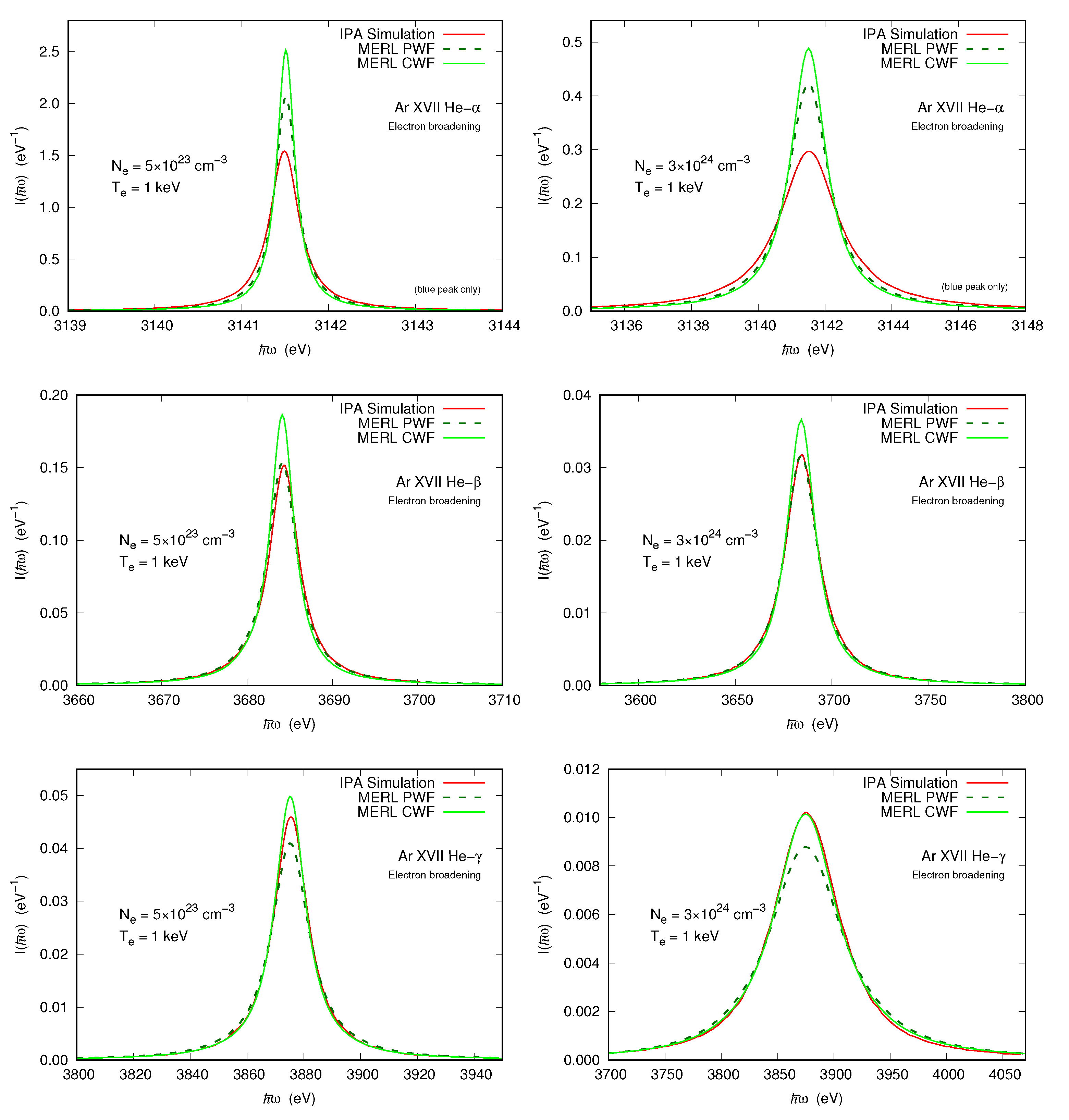
Figure 1 show calculations of the electron broadening function, $J(\omega ,\mathbf{0})$, for $H{e}_{\alpha }$, $H{e}_{\beta }$ and $H{e}_{\gamma }$ line transitions at two electron density values within the range of interest. MERL calculations were done using both PWF and CWF. Results from the IPA simulation are also shown. MD results are not plotted because electron-broadened line shapes cannot be rigorously calculated using MD due its own nature. When considering interacting ions and electrons, their contributions cannot be isolated. For instance, in a MD simulation many electrons indeed closely follow the ions and inherit their slow movement—the correlation between the ion field and the electron one in fact gives rise to the Debye screening. Thus, even though tentative electron-broadened line shapes could be calculated from MD simulations by taking only the electric field generated by the electrons, this field would be in fact affected by the ions. Therefore, the corresponding comparison would not be fair and might lead to ambiguous conclusions.

As seen in Figure 1, MERL-CWF always provides narrower profiles than MERL-PWF. A plausible interpretation could be that the effective electron-radiator interaction time is smaller when using CWFs, the perturbing field correlation decays faster and this leads to a narrower line. On the other hand, since straight-line trajectories are the classical counterpart to PWFs, one would had expected a good agreement between IPA and MERL-PWF. However, results do not show such a regular trend, but a transition-dependent one. For $\alpha$-transitions, both MERL-PWF and CWF lines are narrower than IPA calculations, but for high-n transition lines, e.g., see the plot for He${}_{\gamma }$, MERL-PWF predicts broader line profiles.

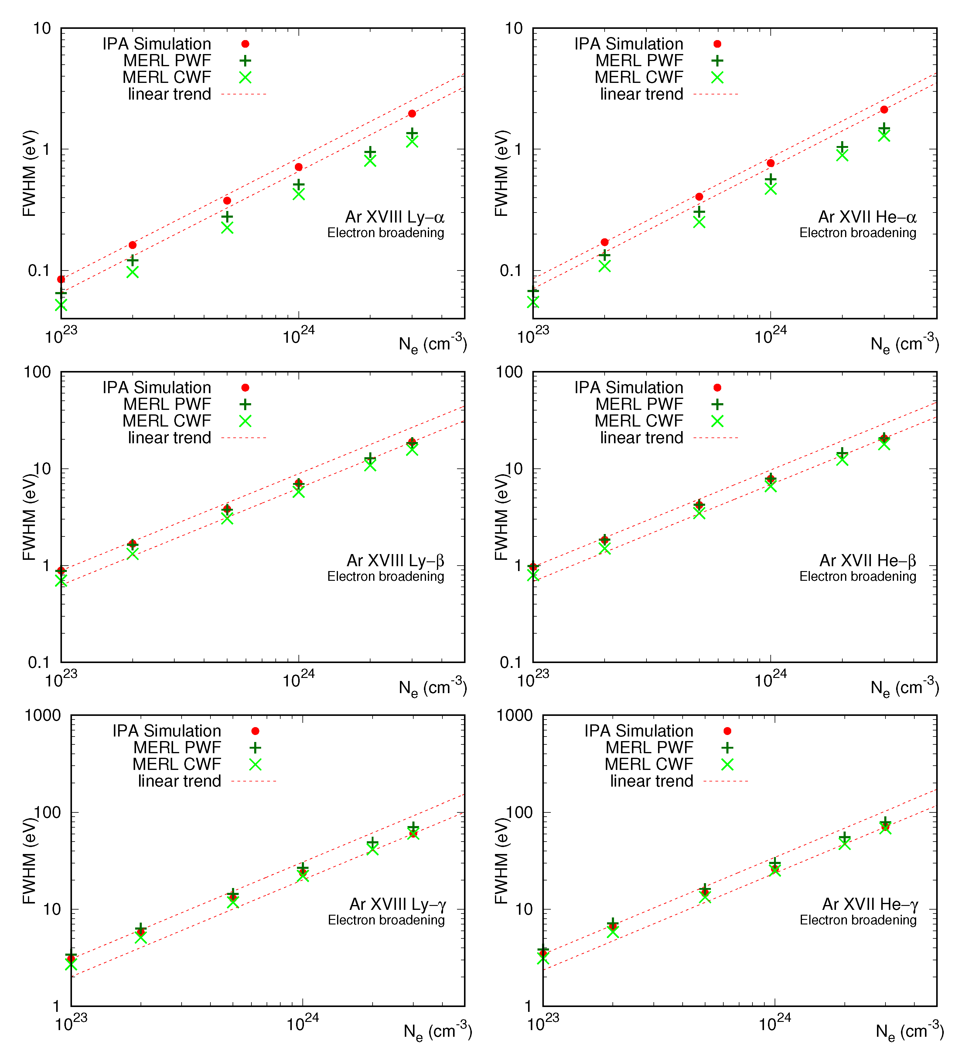
Figure 2 shows the electron-broadening FWHM dependency on electron density for argon He${}_{\alpha }$, He${}_{\beta }$, He${}_{\gamma }$, Ly${}_{\alpha }$, Ly${}_{\beta }$, and Ly${}_{\gamma }$ lines. For the He-like transitions the two fine-structure components, 1snp ${}^1$P${}_1\to$1s${}^2$ ${}^1$S${}_0$ and 1snp ${}^3$P${}_1\to$1s${}^2$ ${}^1$S${}_0$, are well-separated in energy, but the high-energy component, 1snp ${}^1$P${}_1\to$1s${}^2$ ${}^1$S${}_0$, is much more intense, so its line-width can be easily determined. 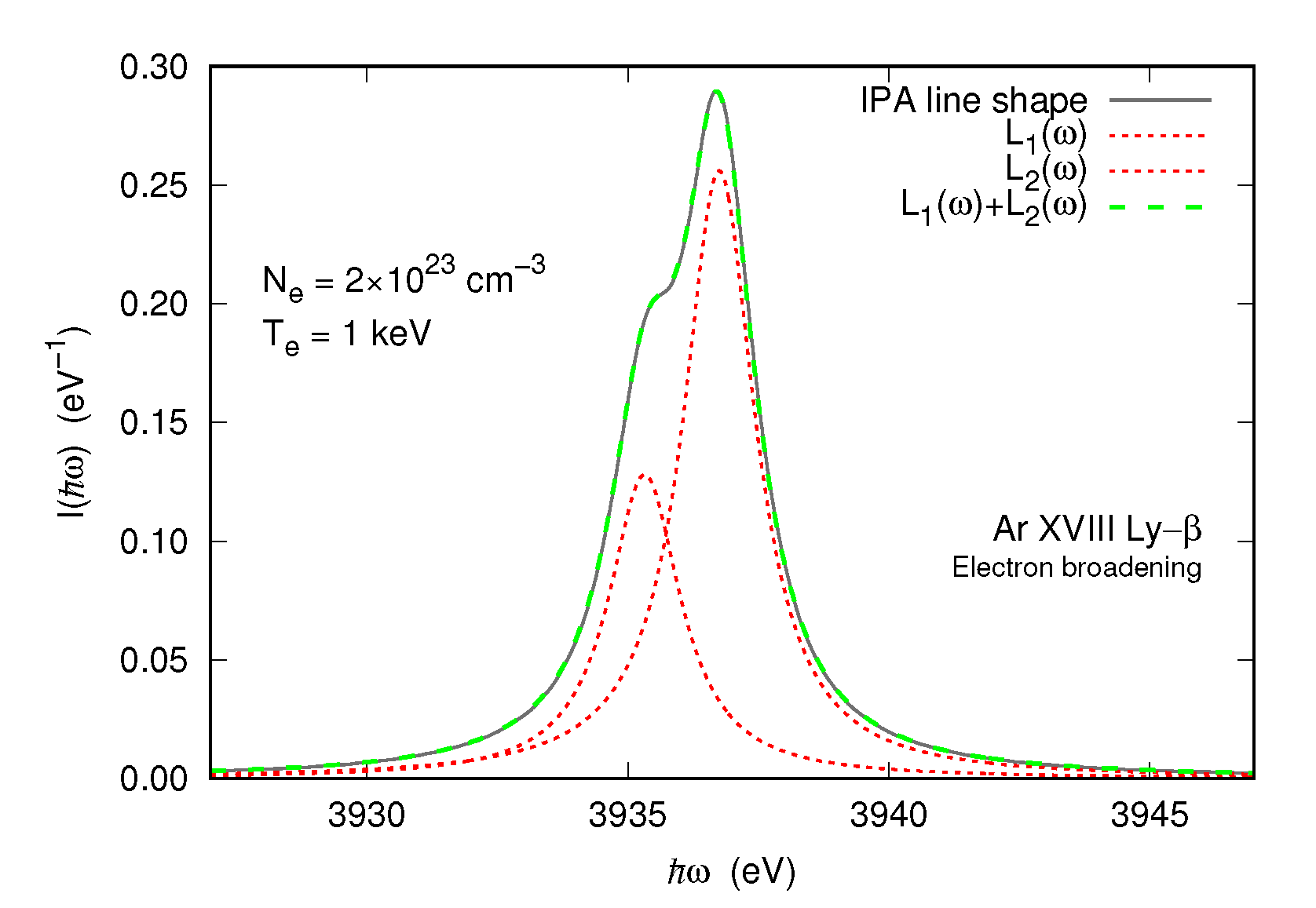For H-like line transitions, the blue component, np ${}^2$P${}_{3/2}\to$ 1s ${}^2$S${}_{1/2}$, is also the dominant one, but their relative intensities are not dramatically different and can significantly overlap for $\beta$ and $\gamma$ transitions at higher density values. For these cases, fitting the line profile using a two-Lorentzian linear combination allowed us to efficiently extract the line-width of each component see Figure 3. For the sake of clarity, only the FWHMs corresponding to the dominant component are plotted in Figure 2. Also, straight lines indicating the strictly linear dependency on electron density have been added for reference. Overall, both IPA and MERL calculations agree well with the following trend: $FWHM\propto N_e^a$, with $a\approx 0.9$. We notice that MERL-PWF slightly deviates from this behavior. In particular, electron broadening calculations from MERL-PWF and IPA show good agreement for $\beta$-transitions over the entire electron density range. This is an important result because, as discussed in Section 3.4, plasma diagnosis based on spectroscopic analysis often relies on relative intensity distribution and line widths of $\beta$ lines to extract temperature and density, respectively.

Interestingly, for a given line transition, the line width (FWHM) ratio between MERL calculations and IPA results remains reasonably constant for the whole density range, therefore the discrepancies between models in the electron broadening treatment are reduced to a factor with a weak dependence on density. This seems clear when one goes deeper into the details for the calculation of the electron broadening operator in MERL. Typically, the $\mathcal{M}(∆\omega )$ matrix elements, see for instance Equation (3) of Ref. [30], factorizes in two terms. The first one expresses the fact that the electron broadening operator scales with plasma conditions as ∼$N_e/\sqrt{T_e}$—which is basically the density-dependency found from our results. The second one, which has a complicated but weak dependency on density, contains the fundamental atomic physics data relative to the state of the atomic system, and, more importantly, a function describing the interaction between the radiator and the perturbing electrons. It is plausible to think that differences between MERL and IPA come from how this latter function accounts for the statistical properties of the time-dependent field produced by the fast-moving electrons.

3.2. Complete Line Shapes

Next we address the comparative study of complete line shapes, i.e., besides the collisional electron broadening, other broadening mechanisms such as the one generated by the quasi-static ion field and ion dynamics effect are now considered. We are particularly interested in investigating the Stark-broadening of line transitions in K-shell Ar ions embedded in a deuterium plasma, since this has been the application scenario of K-shell spectroscopic analysis in multiple ICF direct- and indirect-drive experiments. As deuterium ions are ∼20 times lighter than argon ions, ion dynamics play an important role in this case. We remind that all the referred broadening mechanisms naturally and simultaneously appear in the computer simulations. Additionally, the MD simulation also accounts for the recombination broadening that arises as a consequence of emitter recombination. Further details about this phenomenon are discussed in Section 3.3. Here we restrict to the comparison between different models. Lastly, given the temperature regime achieved in typical ICF plasmas, Doppler broadening must be also considered. For the representative temperature of 1000 eV, characteristic Doppler FWHM value is ≲2 eV.

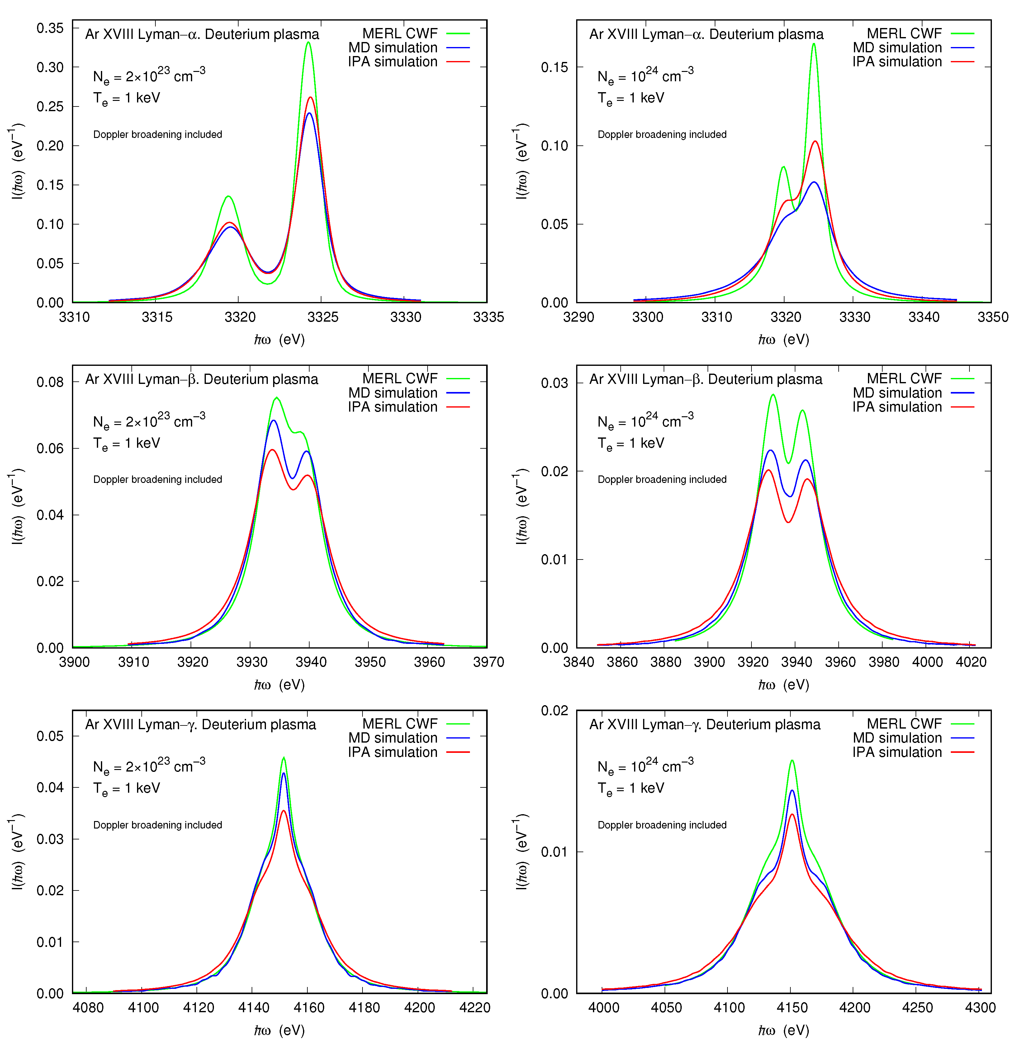
In Figure 4 we present a comparison of complete area-normalized line shapes calculated using MERL-CWF, and IPA and MD simulations for Ly${}_{\alpha }$, Ly${}_{\beta }$, and Ly${}_{\gamma }$ at two representative electron densities. Compared to the electron-broadened ones, profiles show the characteristic structure that appears due to the quasi-static ion microfield, i.e., Ly${}_{\alpha }$ preserves the double-peaked shape from the electron-broadened fine-structure components now further broadened due to the ion microfield effect, Ly${}_{\beta }$ has a distinctive double-peaked shape with a central dip that arises from the Stark energy level splitting and field-mixing, and Ly${}_{\gamma }$ presents an unshifted central peak with two side-shoulders. As expected, for a given transition, line shape broadens as density increases. When comparing different models, MERL-CWF predicts narrower profiles for all the cases. Differences between MERL-CWF line shapes and those provided by simulations are noticeable for $\alpha$ lines and less pronounced for $\beta$ and $\gamma$ transitions, which suggests that the general trend already observed when considering only the electron broadening survives after accounting for additional broadening mechanisms. We also observed that for $\beta$ and $\gamma$ transitions the MD simulation produces narrower line shapes than IPA. The simulation with interacting particles provides electric field statistics shifted to weaker values compared to that resulting from a simulation with non-interacting particles, which leads to narrower spectra in general. However, for $\alpha$ lines, the opposite behavior is observed, i.e., the IPA line shape is narrower than the MD one. This is because the Stark-broadening is indeed much smaller for the $\alpha$ line than for higher-n transitions and therefore the impact of the recombination broadening—which naturally appears in the MD simulation, but does not exist in IPA—relative to the Stark-effect is more pronounced. The Stark-broadening dominates for $\beta$ and $\gamma$ lines, and recombination effect becomes less important. The same qualitative behavior was observed in the complete profiles of He-like Ar line transitions.

3.3. Recombination Broadening

As discussed above, when a free electron is trapped by an argon ion, the line emission process interrupts and the dipole autocorrelation function abruptly drops to zero, which in turn translates into an additional broadening of the line. The criterium to identify an electron trapping was already described in Section 2.1.2. To assess the impact of this phenomenon on the line profiles we carried out two different calculations. The first one indeed corresponds to a standard calculation, and this is why we have emphasized that MD simulation naturally tackles the recombination process. Within a classical picture, the MD code solves the plasma particle dynamics including the argon ions. Each simulation run provides multiple time-histories of the electric microfield, $\mathbf{E}\left(t\right)$, perturbing a given argon ion. In a simulation run at given plasma conditions the time-histories are computed till a time T greater than the average correlation-loss time of the emitting dipole, i.e., $\left\{C\left(T\right)\right\}\approx 0$, with $\left\{\cdots \right\}$ denoting the average over the statistical ensemble. Field time-histories are stored and then used to solve the Schrödinger equation, Equation (3), to ultimately computing the dipole autocorrelation function. If over a particular time-history, $\mathbf{E}\left(t\right)$, recombination occurs, such sequence is terminated, but still considered on the same footing with the remaining time-histories to proceed with the line shape calculation. For the second calculation, field time-histories affected by an electron trapping are removed and the average autocorrelation function is computed using only field sequences seen by non-recombining ions.

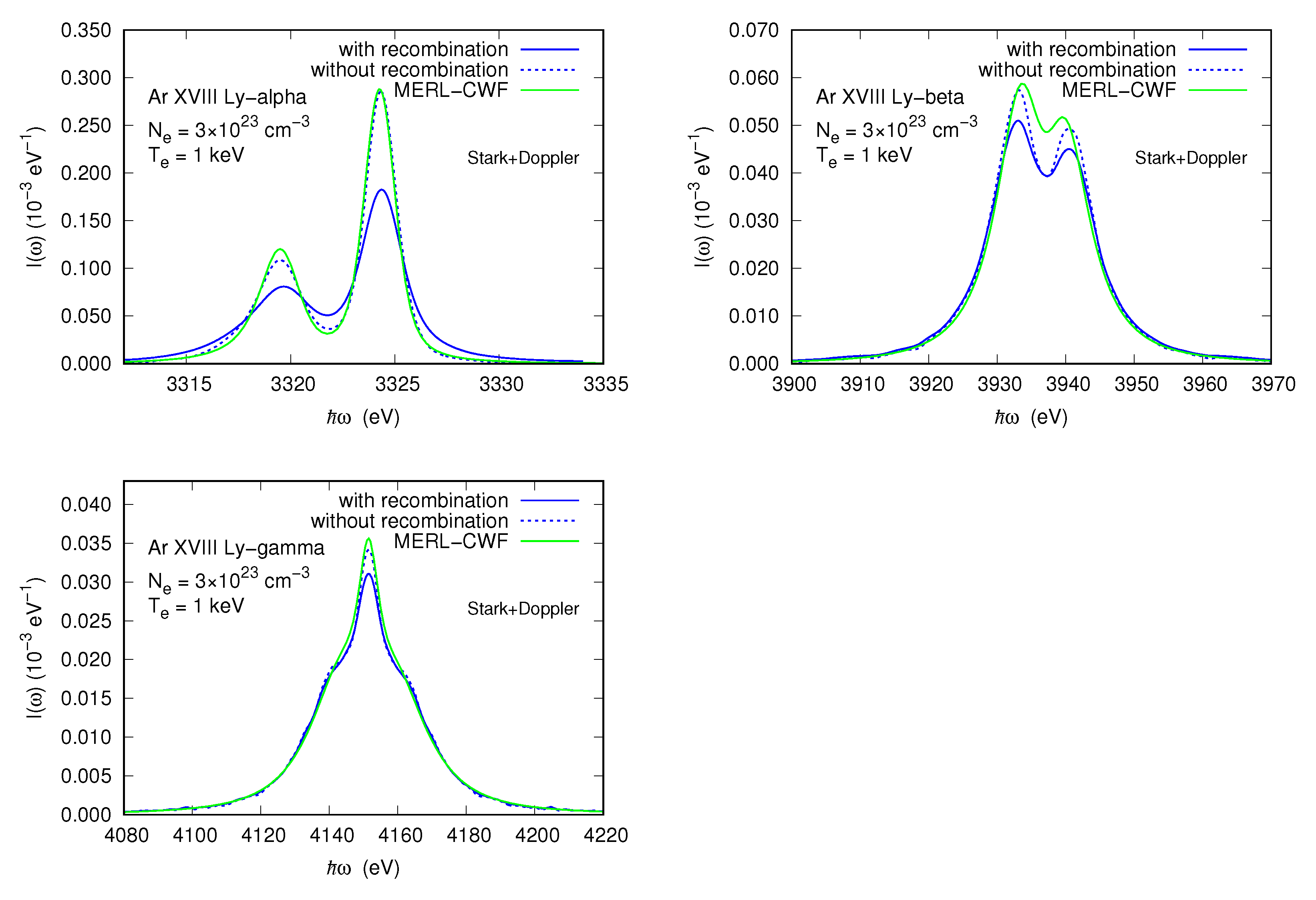
Figure 5 shows line shapes computed with and without the recombination broadening for H-like Ar transitions, i.e., Ly${}_{\alpha }$, Ly${}_{\beta }$, and Ly${}_{\gamma }$, at $N_e=5\times {10}^{23}$ cm${}^{-3}$. Similar qualitative results were found for He-like lines and different density conditions. The electron trapping gives rise to a broadening mechanism to be added to the Stark-broadening. Conceptually, this phenomenon can be described in terms of the standard Lorentz model, where the line width represents a measure of the rate of atomic processes that abruptly produce a coherence break. Within a classical framework, the recombination rate does not depend on the emitter internal state—there is no such distinction when simulating the particle dynamics—and therefore within the same ion stage the recombination broadening does not depend on the line transition. In this context, if the Stark-broadening is rather small for a particular line, then the additional recombination broadening can be relevant and should be taken into account for an eventual spectroscopic analysis, e.g., this is the case of Ly${}_{\alpha }$. For lines affected by a strong Stark-broadening, this phenomenon becomes less important, as happens for $\beta$ and $\gamma$ transitions.

In this regard, a recent work [8] emphasized the role of electron-capture (EC) on spectral line broadening in hot dense plasmas. It is important to note that here EC refers to the atomic process that occurs when a free electron is captured by an ion, i.e., recombines, and after some energy distribution the recombined ion ends up in a doubly excited or autoionizing state. Another well-known recombination process is the three-body recombination (3BR), i.e., two electrons enter at the same time into the volume of one ion and one of the two is captured in a bound state, whereas the other takes up the extra energy [31]. In the case of our classical MD simulations, the observed recombination process has not—if any—a clear quantum-mechanical counterpart. This is why we pointedly have referred to it simply as recombination or electron trapping, thus eluding a straightforward association with either EC or 3BR. Since the MD simulation does not include dissipative radiative processes, the classical recombination cannot account for the radiative recombination process, so it would rather represent a joint effect due to EC and 3BR. In Ref. [8] authors point out that EC might have a significant effect on $\alpha$ lines, but negligible for higher-n transitions, which would be due to the reduced number of EC channels and weaker interaction with increasing n. Interestingly, our results show the same qualitative behavior. Moreover, we notice that MERL calculations—where no recombination process was included—agree better with the MD line shapes without recombination broadening. Further investigations are needed to answer the open questions on this topic. Here we limit ourselves to report the performed calculations and to warn about the impact of recombination broadening on the line shapes.

3.4. Impact of Stark-Broadening Models on the Spectroscopic Diagnosis of OMEGA Implosions

The differences in the line shapes discussed in the previous section motivate the question of how much the use of different line shape codes may impact a spectroscopic diagnosis analysis. To investigate this issue, we performed the analysis of time-resolved Ar K-shell spectra recorded in direct-drive implosion experiments conducted in OMEGA [32]. The experiments consisted of imploding spherical plastic shells which had an initial diameter of 435 $\mathsf{\mu }$m, wall-thickness of 27 $\mathsf{\mu }$m and an outer Al sealing layer of 0.1 $\mathsf{\mu }$m. They were filled with 20 atm of D${}_2$ and a tracer amount of Ar, 0.072 atm, for spectroscopic purposes. The emission from Ar K-shell lines becomes bright at the collapse of the implosion, when the imploded core temperature reaches the keV-range and electron density increases above 10${}^{23}$ cm${}^{-3}$. An X-ray streaked spectrometer with a spectral resolving power $E/∆E\approx 500$ was fielded in order to record the time-resolved space-integrated spectrum spanning the photon energy range from 3000 to 4300 eV.

The model to analyze the data consists of a spherical plasma source with uniform electron temperature, $T_e$, and density, $N_e$, representing the imploded core. The core radius R can be determined from $N_e$ assuming mass conservation. For such geometry the radiation transport equation can be analytically integrated, and the emergent intensity distribution $I\left(\omega \right)$ is given by [33]

$$I\left(\omega \right)=\pi R^2\frac{\epsilon \left(\omega \right)}{\kappa \left(\omega \right)}\left\{1+\frac{e^{-2\kappa \left(\omega \right)R}}{\kappa \left(\omega \right)R}-\frac{1-e^{-2\kappa \left(\omega \right)R}}{2{\left[\kappa \left(\omega \right)R\right]}^2}\right\},$$

(12)

where $\omega$ is the angular photon frequency, and $\epsilon \left(\omega \right)$ and $\kappa \left(\omega \right)$ stand for the temperature-, density- and frequency-dependent emissivity and opacity of the core. The required emissivities, opacities and atomic level population distributions were calculated with the collisional-radiative atomic-kinetics model ABAKO [34] over a sufficiently wide range of temperatures and densities. All bound-bound, bound-free and free-free contributions from the Ar-doped deuterium plasma within the data spectral range were included. In particular, bound-free cross-sections were calculated with the LANL suite of codes [29].

For this application an ABAKO model for argon was constructed including up to 4592 energy levels from fully stripped through C-like Ar. Energy levels and line transition rates were computed with the atomic structure code FAC under the relativistic-detailed-configuration-approach (RDCA), including unresolved transition arrays [35] and configuration interaction corrections. The current version of ABAKO includes a module that automatically executes FAC to compute the energy level structure and related fundamental atomic data to subsequently build the collisional-radiative matrix ensuring state-space completeness for the corresponding application. Other than that there is no particular reason for using either FAC, Cowan’s or similar codes. There is no inconsistency in using FAC for the atomic kinetics and Cowan’s data for line shape calculations. Note in turn that, in this work, when computing the emergent spectra using different line shape models, the atomic kinetics model remains indeed the same. Therefore, different results will be only due to the distinctive features of Stark-broadening models. Moreover, for line shapes calculations, populations of fine-structure levels belonging to the initial state were assumed to distribute according to their statistical weights (for the case of IPA and MD simulations) or to follow the Boltzmann statistics (MERL calculations). For the application discussed here, in the context of hot dense plasmas, these assumptions are both equivalent and well-justified: (a) collisional processes domain the relative population distribution among fine-strcuture levels, and (b) characteristic temperatures are much greater than energy differences between fine-structure levels, i.e., $∆E/T_e\ll 1$.

For given plasma conditions, ABAKO explicitly includes all non-autoionizing and autoionizing states consistent with the corresponding ionization potential depression, which is estimated according to the Stewart-Pyatt model [36], modified to account for the argon-deuterium mixture. An escape factor model was used to account for radiation trapping effects on the atomic-level population kinetics [37].

Importantly for this investigation, Stark-broadened line shapes for Ar $H{e}_{\beta }$, $H{e}_{\gamma }$, $L{y}_{\beta }$ and $L{y}_{\gamma }$ were calculated for density values from ${10}^{23}$ to $3\times {10}^{24}$ cm${}^{-3}$ using three different models: MERL-CWF, and the IPA and MD computer simulations. Since line shapes sensitivity with temperature is small, all calculations were done at the representative value of 1 keV. Synthetic spectra also include detailed Stark profiles for Li-like satellites of $H{e}_{\beta }$ ($1s3p\mathrm{n}l\to 1s^2\mathrm{n}l$) and $H{e}_{\gamma }$ ($1s4p\mathrm{n}l\to 1s^2\mathrm{n}l$), and He-like satellites of $L{y}_{\beta }$ ($3p\mathrm{n}l\to 1s\mathrm{n}l$); however due to the high computational demand of simulation models, only MERL-CWF was used to calculate the line shapes of satellite transitions. This fact does not override our study on model dependence because, although satellites are needed for better modeling the observed spectra, the analysis results mostly rely on the representation of the corresponding parent lines.

Furthermore, for the plasma conditions of these implosions, characteristic optical depth values $\tau$ for argon line transitions are: $\tau \sim 0.5$ for the $H{e}_{\gamma }$ and $L{y}_{\gamma }$ lines, $\tau \sim 1$ for the $H{e}_{\beta }$ and $L{y}_{\beta }$, and $\tau >10$ for the $H{e}_{\alpha }$ and $L{y}_{\alpha }$. Therefore, besides the intrinsic difficulties for properly modeling the profiles, $\alpha$ lines are much more sensitive to spatial gradients and absorption effects than others. This is the reason why density diagnostics based on K-shell spectroscopy usually rely on the $\beta$ and $\gamma$ lines region of the spectrum. Accordingly, the analysis of the time-resolved Ar K-shell spectra measured in the OMEGA implosions was carried out for the photon energy interval from 3500 to 4300 eV, thus including $H{e}_{\beta }$, $H{e}_{\gamma }$, $L{y}_{\beta }$ and $L{y}_{\gamma }$ lines. Thus, despite the discrepancies observed between MERL and simulation results on the $\alpha$ line shapes, the study of spectroscopic analysis dependence on line shape models turns into an assessment of the impact of differences observed in $\beta$ line shapes, and $\gamma$ ones to a lesser extent.

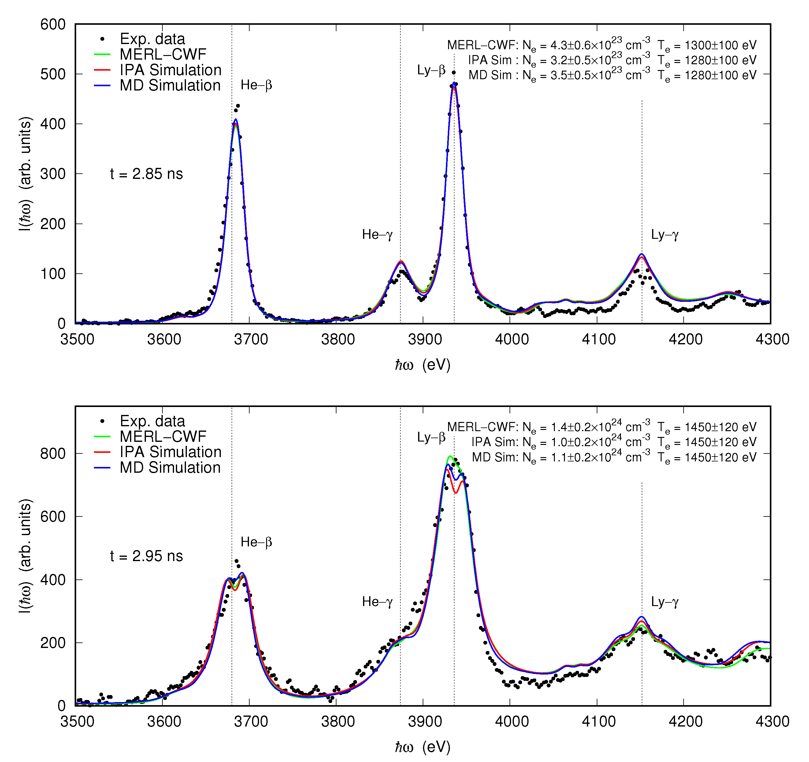
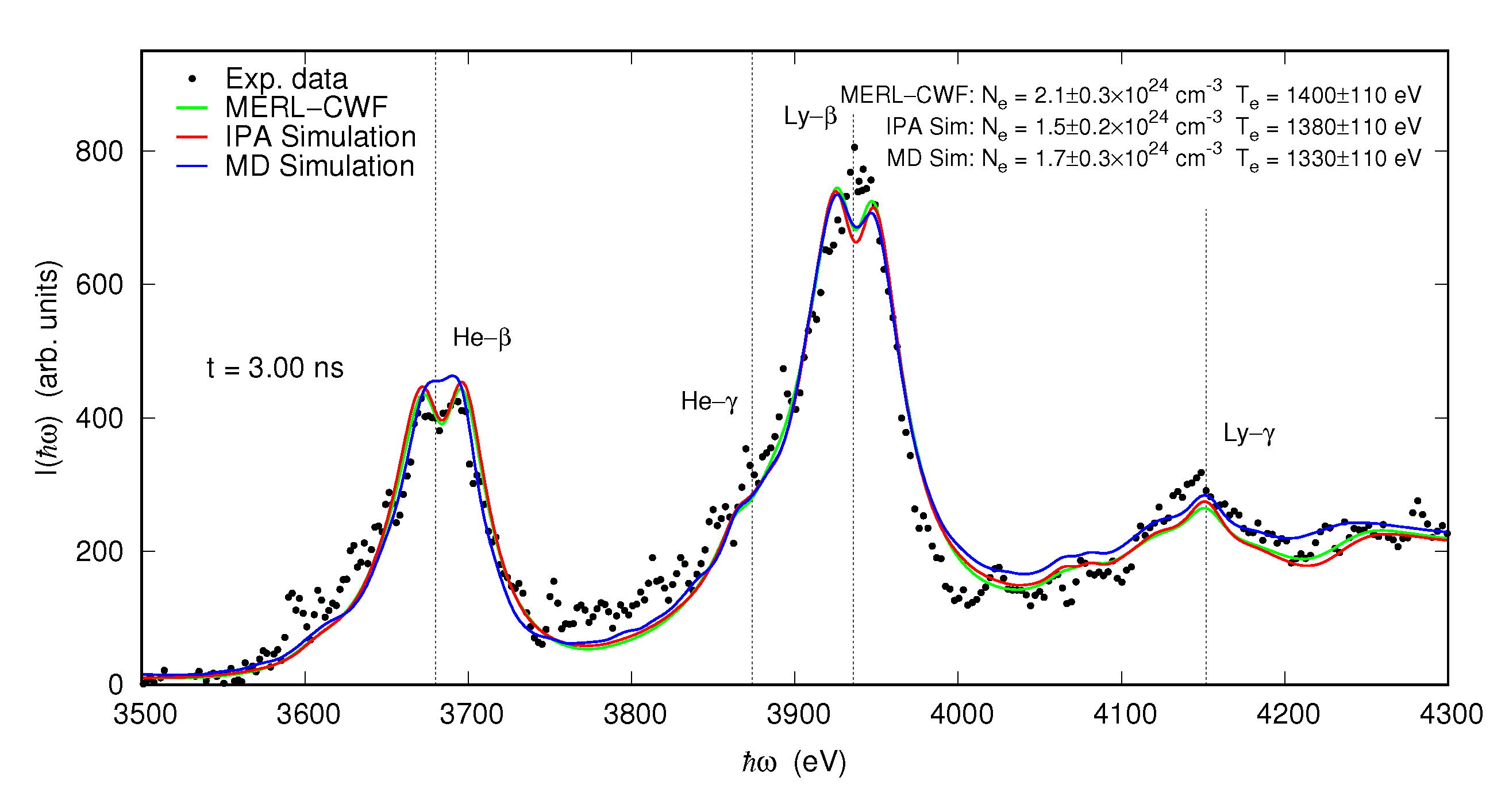
As an illustration, Figure 6 shows the analysis of three time-resolved spectra recorded in OMEGA shot 49956 from earlier to later times through the collapse of the implosion. For this application, we used ABAKO and the three referred line shape models to build three databases of $40\times 55$ synthetic spectra—following Equation (12)—on the intervals $\left[1000,2000\right]$ eV and $\left[{10}^{23},3\times {10}^{24}\right]$ cm${}^{-3}$ for electron temperature and density, respectively. For each model, an exhaustive search on the two-dimensional parameter space following a weighted-${\chi }^2$ minimization procedure was done to find the best model fit and confirm that a single global minimum was found. As seen, the three models were able to produce good fits to data (with ${\chi }^2\sim 1$) and extracted conditions are consistent with the implosion dynamics and analysis discussed in previous works [38,39]. Extracted temperature values are very similar. This is because temperature sensitivity mainly depends on the relative distribution of line intensities through temperature-dependent population densities and the atomic kinetics model remains unchanged in the three calculations discussed here. Density sensitivity mostly relies on Stark-broadening of the line shapes, so greater differences between models are found in the extracted density values. MERL-CWF always yields higher densities, while IPA simulation the lowest ones. This agrees with the results found in the previous section, where for a given density value, MERL-CWF produced the narrowest line shape and IPA the broadest one. Relative to MD simulation results, extracted densities are ∼25% higher for MERL-CWF and ∼10% lower for IPA. This level of discrepancy agrees with the one reported in several works for different line shape models and methods [6,7]. To quantify to what extent these discrepancies reveal an impact on K-shell spectroscopy, one needs to take into account the inherent uncertainties in the data analysis. Statistical uncertainties in the parameters associated with the minimization procedure were computed as the standard confidence limits on temperature and density, which in turn result from a curvature analysis of the two-dimensional weighted-${\chi }^2$ surface about the minimum, taking into account the correlation between the parameters. Additional uncertainties come from the data-processing itself (mainly from the subtraction of background continuum emission, which is applied to the experimental spectrum before the comparison with the synthetic spectra) [32]. Accounting for all these factors, we estimated a total uncertainty of ∼8% in temperature and ∼15% in density. Therefore, extracted temperature values are clearly within uncertainties. Results of density diagnosis using both simulation models are likewise indistinguishable considering the data analysis uncertainty. On the other hand, density values extracted from MERL-CWF and those determined from the simulations overlap at about the limit of the corresponding uncertainty intervals. In conclusion, our analysis minimizes the impact due to the use of different line shape models on the K-shell spectroscopy analysis of implosion experiments at OMEGA, and validate the results obtained by either of the three models discussed here.

4. Conclusions

Atoms and ions in a plasma are subject to strong interactions with their environment and therefore the analysis of the emitted or absorbed radiation provides information about the plasma conditions. In particular, Stark-broadening, i.e., broadening of spectral lines as a result of the emitter being perturbed by the electric field due to surrounding ions and electrons, is currently used as a non-intrusive technique to diagnose the density in hot dense plasmas. However, some persistent discrepancies between measurements and models and the lack of independent measurements in the high density regime have stimulated new research in the line broadening theory. In this context, computer simulations are often considered to be idealized computational experiments for benchmarking and improvement of theoretical models. In this work, we performed a cross-comparison study of Stark-broadened line shapes using the well-known Multi-Electron-Radiator-Line shape code (MERL) as well as computer simulations with (a) non-interacting and (b) interacting particles. We focused on K-shell X-ray line transitions in He- and H-like argon ions, since these lines have been extensively used for the characterization of imploding cores in ICF-related experiments. Reported differences between MERL and simulations are basically due to the distinctive treatment of the electron broadening mechanism, and become more pronounced for the $\alpha$ lines, i.e., $n=2\to n=1$ transitions. Also, we discussed the impact of the recombination broadening—that naturally appears in interacting-particle simulations as a consequence of the classical ionization-recombination mechanism—on line shapes and reported on similar qualitative results recently published using quantum collision theory. Finally, we assessed the impact of employing either molecular dynamics (interacting-particles) or MERL line profiles on the diagnosis of core conditions in implosion experiments performed on OMEGA. Differences in extracted conditions when using different line shape models are not significant when data analysis uncertainties are considered, thus minimizing the model-dependency of the K-shell spectroscopy analysis. However, since extracted density values may differ as much as ∼20%, caution is advised for application in other HEDP scenarios. Further investigation is in progress to clearly identify the reasons causing the reported discrepancies between models and will be published elsewhere.