
EUV Beam-Foil Spectra of Scandium, Vanadium, Chromium, Manganese, Cobalt, and Zinc


AIRUB, Fakultät für Physik und Astronomie, Ruhr-Universität Bochum, 44780 Bochum, Germany
Atoms 2021, 9(2), 23; https://0-doi-org.brum.beds.ac.uk/10.3390/atoms9020023
Submission received: 27 February 2021
/
Revised: 22 March 2021
/
Accepted: 25 March 2021
/
Published: 29 March 2021
(This article belongs to the Section Atomic, Molecular and Nuclear Spectroscopy and Collisions)
Abstract
:Beam-foil extreme-ultraviolet spectra of Sc, V, Cr, Mn, Co and Zn are presented that provide survey data of a single element exclusively. Various details are discussed in the context of line intensity ratios, yrast transitions, delayed spectra and peculiar properties of the beam-foil light source.
1. Introduction
The selection of elements subjected to laboratory spectroscopic study is influenced by the interests of the data user community. In the 1960s and 1970s, there was a particular interest in atomic data for controlled nuclear fusion experiments. While fusion actually aimed at hydrogen and helium, the practical interest in heavier elements was in the avoidance of contaminations, such as by the elements used for the production of stainless steel vacuum vessels. Therefore, funding supported laboratory spectroscopy for iron group elements up to Ni (); this bias and limitation is still reflected in the holdings of spectral databases. A second field of interest arose at the same time from Skylab and other satellites that carried extreme ultraviolet (EUV) and X-ray spectrometers beyond Earth’s atmosphere. Researchers marvelled at the rich EUV and X-ray spectra of the solar corona. Brian Fawcett, Alan Gabriel, Carole Jordan and their colleagues recognised that a study of both terrestrial and astrophysical light sources might be mutually beneficial [1,2,3]. Astrophysics was interested in the same EUV spectra, in particular of the most abundant elements. Because of nuclear physics reasons ( clustering in nuclei), the elements with even atomic numbers are much more abundant than the odd-numbered ones. Consequently, Ti (), Cr (), Fe () and Ni () have been studied for their spectra much more than Sc (), V (), Mn () and Co (). However, the even-numbered elements Cr and Zn () have been studied much less extensively than Ti, Fe and Ni (which, along with Cu, are considered for a future presentation), and therefore Cr and Zn have been included in the present data sample along with the odd-numbered elements of the iron group.
The early wavelength compilation by Kelly and Palumbo [4] has been updated in various formats, of which the work in [5] appears to be the most recent one. According to author Kelly [4], the wavelength data for the compilation were selected on the merit of their apparent precision, but without a dedicated atomic structure analysis. The US National Bureau of Standards (NBS), later reconfigured as the National Institute of Standards and Technology (NIST), began systematic tabulations (with term analysis) in the 1940s, often relying on in-house spectroscopic work of high quality [6]. Their data holdings nowadays are available as the NIST ASD online database [7]. Quality assurance, however, is tedious and time-consuming. Consequently, at times some sections of the database were much slimmer than the corresponding Kelly tables. Other sections were much thicker, as the wavelength coverage of the NIST tables was not confined to the vacuum ultraviolet (VUV) as were the original Kelly and Palumbo tables. The NIST ASD tables list lines, levels and many transition rates. The latter most often are not obtained from experiment, but from computations, as is a sizable fraction of the spectral data nowadays. (This has advantageous and worrying aspects.) Another database of widespread interest is the result of the CHIANTI project [8,9,10,11,12]. This work addresses primarily astrophysicists and their needs; the objectives, achievements and perspectives of the CHIANTI project have recently be reviewed by project members [13]. Computed EUV spectra (modelled for various electron densities and temperatures as occur in the solar corona) help with the analysis and understanding of stellar spectra. For reasons already mentioned, the emphasis is on the spectra of elements abundant in the Sun. This interest puts the odd-numbered iron group elements largely aside (see the CHIANTI coverage overview in [13]).
Atomic structure computations of the levels and transition wavelengths have massively improved over the decades. Fawcett provided some of the earliest wide-range tabulations on levels, wavelengths and transition rates [14] that intended to systematise his extensive observations by way of scaled Hartree–Fock computations. The results of this technique are not very precise on their own, but by an adjustment of Slater parameters the computations can practically be fitted to the observational data and thus the consistency of the data be checked at a high-quality level [15]. A number of atomic structure computations have addressed short or long sections of various isoelectronic sequences; they are too many to list here, especially as the progress of such computations implies that there are many earlier attempts that may have done well for their time (and some remain among the excellent few), but most have been superseded since. Examples of recent high-accuracy computations on isoelectronic sequences that include ions of present interest (isoelectronic sequences F, Ne, Mg, Si and S) can be found in [16,17,18,19,20,21,22,23,24,25,26,27] and the references cited therein. The status of atomic structure calculations reached nowadays, employing ab initio computations following various approaches, has been discussed recently by Jönsson et al. [28].
Half a century after Fawcett and Gabriel’s trailblazing studies, it may be appropriate to help filling some of the gaps in the knowledge on the less-studied elements. For this purpose, I have retrieved some of my own beam-foil spectra from storage. The recordings were made at the Bochum tandem accelerator laboratory a quarter century ago, starting out with straightforward observations of electric dipole (E1) transitions, decay curves of regular and displaced terms, and various isoelectronic studies of specific configurations. For examples of such work on elements of present emphasis see in [29,30,31,32,33,34,35,36,37]. From this field of activity evolved a quest for finding spin-changing intercombination lines in iron group ions with an open valence shell, and for measuring their transition rates (see, for example, in [38,39,40,41,42,43]). These and various other investigations have concentrated on certain wavelength intervals in the EUV. In order to ascertain the measurement situation and to gain a perspective on the spectra under study, survey spectra were recorded for most elements before turning to detail spectra. It is these surveys that I want to preserve for public access, so that other researchers can use them for their orientation. A number of detail spectra are to be shown as well, supplemented by explanations of why I consider them noteworthy.
Of course, the work at Bochum was not singular in Europe, where accelerator-based atomic physics was pursued in many laboratories (to name a few, Aarhus, Berlin, Copenhagen, Darmstadt, Kaiserslautern, Liège, Lund, Lyon, Munich, Oxford, Stockholm and Uppsala), nor in North America (with numerous US American and Canadian laboratories). It just happened that the accelerator type (selected for certain nuclear physics experiments) and ion source capabilities at Bochum turned out to be eminently suitable for atomic physics studies of many elements in the first third of the sequence of the elements. Because of the versatility of the facility, not only elements of primary general interest could be studied, but also those that found less interest elsewhere, but are useful for the systematics.
2. Beam-Foil Spectra
The beam-foil measurement technique has been recalled in a recent companion paper [44] and various reviews (see in [45,46] and references therein). The spectra shown in this study have been obtained at the Bochum Dynamitron tandem accelerator laboratory (DTL), where a 4 MV tandem accelerator equipped with a sputter ion source [47,48] provided ion beams of an energy between a few MeV up to about 30 MeV with beam currents (particle current) in the range from 0.01 A to about 1 A of the iron group elements. The ion beam with its typical velocity of about 1 cm/ns (roughly 3% of the speed of light) was passed through a thin carbon foil of areal density 10 g/cm, in which it lost a small fraction of its energy. A grazing-incidence spectrometer (McPherson Model 247) equipped with an m grating of groove density 600 ℓ/mm dispersed the EUV radiation emitted by the excited ions. A channeltron served as the detector behind the exit slit of the scanning instrument. The charge state distributions mentioned below refer to various investigations [49,50,51].
The spectroscopic data presented below are ordered by element in the order of ascending atomic number. Various spectral features have been studied in isoelectronic sequences, and specific results have been published elsewhere, usually without showing the survey data in which the details were embedded. Consequently some topics return a number of times in the report below. However, the arrangement chosen here was deemed to make access easier for the reader.
2.1. Sc
A companion paper on K and Ca [44] has reported on a line ratio measurement in the F-like ion K XI, on the line doublet 2s2pP – 2s2pS. The beam-foil line ratio in K XI agreed with the expected value calculated from the wavelengths of the two decay branches of the same upper level, or from computed transition rates [7,11,16]), whereas the corresponding ratios observed in a low-pressure plasma discharge with Ar and Ca [52] did not. The latter fact was interpreted as an indication of an unidentified line blend of the shorter-wavelength component. Beam-foil observations of Sc offer another chance at such a measurement. Figure 1 shows spectra of the wavelength interval 12.5 nm to 15.2 nm. The lines of interest lie at wavelengths 13.0955 nm and 13.7796 nm, respectively [7]. The upper spectrum has been recorded with the rear side of the exciter foil in view as well as the first about 80 ps of the decay, whereas for the lower spectrum the foil has been moved 5 mm upstream, so that the observation represents a time window of about 100 ps width at a mean delay time of about 550 ps after excitation. For the line ratio of two decay branches of a single upper level, the delay does not matter, but, of course, the signal is higher in the beginning. The raw signal ratio is about 2.56, which needs to be corrected for the steep slope of the spectrometer detection efficiency curve [53,54]. The corrected observed line ratio is 2.80 ± 0.40, which is roughly compatible with the NIST expectation of 2.35 and with the value of 2.33 predicted by Jönsson et al. [16].
The weaker line of the doublet lies close to a line that the NIST ASD tables list as Sc XI 3d–4f (transition array at about 13.83 nm); there is another such transition at 15.0939 nm [7], Sc X 3s3d–3s4f. The fine structure intervals of the 3d–4f transition arrays are not resolved here. The Sc X 3s3d–3s4f transition is partly blended with the strongest component (–)) of the Sc XIV 2s2pP–2s2pP multiplet. The lines mentioned so far comprise the four brightest lines in the “prompt” spectrum in Figure 1. In the “delayed” spectrum, the situation has changed and shows the Sc XI 3d–4f transition array at 13.83 nm as the brightest line by far. The Sc XIII line doublet is still present, but rather weakly. Naively, one might assume that the Sc XIII 2s2pS level is shorter lived than the Sc XI 3d level and thus has largely died out. Actually, the lifetime predictions for this level range from 12.3 ps [7] to 15.2 ps (according to RCI computations by Jönsson et al. [16]); unfortunately Aggarwal’s computations of F-like ions [55] have left out Sc XIII. The Sc XI 3d level lifetime has been predicted at about 4.6 ps [7] or, from a simple hydrogenic system estimate, about 4.9 ps. Evidently, the lifetime ratio appears to be “wrong”, and a different explanation is required.
Both level lifetimes are much shorter than the delay time elapsed before the observation of the lower spectrum in Figure 1. Consequently, by the time of this observation, both levels should have been completely depleted and their decays not seen at all—unless the decays observed are repopulated by decays from higher-lying levels. The Sc XIII 2s2pS level is “displaced”, and there is a vacancy below the valence sub-shell. Higher-lying levels that can feed this level would most likely have the same vacancy, which renders them more unstable than regular levels. Furthermore, the transition energies of decays “from high” to this level are smaller (and thus the rates lower and the branch fractions smaller) than for transitions to the ground configuration (parity permitting, of course). Therefore, such displaced levels receive rather little cascade repopulation. The other level, Sc XI 4f, is quite different. It is fed along the “yrast” chain of levels of maximum angular momentum ℓ for each value of the principal quantum number n. (The designation “yrast” follows a custom in nuclear physics.) Those yrast levels in Sc XI have approximate lifetimes of 16 ps (5g levels), 42 ps (6h), 92 ps (7i), 183 ps (8k) and so on. Once a decay path has reached the yrast line, there are no branchings, and all further decays follow the same path. Such a cascade chain easily explains the observed high line intensity of the Sc XI 3d–4f transition even after a considerable delay. In this case of a Na-like ion (closed-shell electron core), the valence electron can be treated well in a hydrogenic approximation, and the line shows little fine structure splitting. Such yrast transitions and their cascades are helpful in beam-foil spectroscopy to provide (moderate quality) wavelength references that can be calibrated with known reference lines in prompt spectra and can carry this wavelength into delayed spectra where wavelength references are scarce. Table 1 lists a number of such yrast transitions and their estimated wavelengths in a simple hydrogenic model approximation. For levels of maximum angular momentum ℓ = , the hydrogenic model estimate is often surprisingly accurate, on the order of 0.01 nm. Many of these lines appear in the spectra discussed below.
In more complex ions, the valence electron behaves grossly similarly to the one-electron case, but the interaction with the structured electron core multiplies the number of components of each transition array. An example will be shown below.
Figure 2 shows a Sc survey spectrum at a relatively low ion beam energy of 9 MeV. Expected charge states are mostly q = 6+ to 11+, with the highest yield for [51]. The strongest lines in this spectrum arise from the Sc XI 3p P–3d D transitions at = 37.2939 nm and 38.1577 nm, respectively, and from the resonance transition in the Mg-like ion, Sc X 3sS–3s3p P at 42.263 nm [7]. The Sc X multiplet 3s3p P–3pP in the wavelength range 45 to 47 nm offers an example of approximate LS coupling, in which case the line intensity patterns of transition multiplets can be estimated from first principles [56]. The line near 40.0 nm likely results from a blend of Sc IX and Sc XII lines. The Sc X 4f–5g yrast transition array is expected (see Table 1) near a wavelength of 40.5 nm, but the characteristic hump of such partly resolved transition arrays is not seen. Because of the interaction of the valence electron with the core, the actual wavelength should be slightly shorter than predicted in the hydrogenic approximation and may be blended with the line blend at 40.0 nm. A higher-resolution spectrum obtained at a higher ion beam energy and presented in Figure 3 contains several small features outside that known line blend, at wavelengths of 40.03 nm and 40.23 nm, which may belong to that yrast transition array. The line at 41.7 nm coincides in wavelength with a transition in Sc XIII [36], but the charge state is not expected to be sufficiently abundant here.
Figure 3 shows beam-foil spectra of Sc of the wavelength interval 38 to 40.3 nm at relatively low ion beam energies. Moderate ion beam energy variations help with identifying the composition of line blends. The lower spectrum indicates (as expected) a higher yield of Sc IX at the lower ion beam energy, while the contributions by Sc XII are much weaker. The primary wavelength reference line at 38.1577 nm is one of the prominent Sc XI (Na-like) 3p–3d transitions.
At an ion beam energy of 23 MeV, the expected range of charge states after passing the beam through a thin foil is to 14+, with the maximum fraction belonging to [51]. The spectrum in Figure 4 was recorded to obtain a second diffraction order image of the data range of Figure 1. This is, both a method to obtain spectra at doubled spectral resolution and to gain wavelength references in a spectral range short of calibration lines. Although the wavelengths of a line pair at 26.2 nm and at 27.6 nm are close to twice those of the Sc XIII line pair, the agreement is not perfect, and the weaker line of the pair falls close to a group of lines of uncertain origin (see below). Second diffraction order images have been seen with the diffraction grating used, but only rather weakly in most parts of the working range. In corresponding observations on Ti ions (an element differing from Sc by one unit of atomic number and thus with corresponding spectral features close by in wavelength) the evidence speaks clearly for the appearance of the two second-order lines of the F-like spectrum under the present working conditions. Thus at least the Sc XIII 2s2pP–2s2pS ( 13.0955 nm [7]) can serve as a reference line in second diffraction order (m = 2 × 13.0955 nm = 26.1910 nm) in this data set. The weak branch of the same multiplet is present, too, but it is tainted by a near coincidence with uncorroborated neighbours.
The lines in the wavelength interval 27.3 nm to 28.1 nm have not been identified yet. They might, as a minor contribution, comprise the Sc XII 4f–5g yrast line cluster. For Sc, this wavelength range has been covered in only a single measurement. The wavelength pattern and the line widths of the unidentified lines are compatible in principle with regular data, but no such line cluster is expected in this position, in the wide gap between most of the – and the majority of transitions. Therefore, the spectral feature in the wavelength interval 27.3 nm to 28.1 nm may, for example, be an artefact caused by damages to the exciter foil (small holes developing under ion irradiation); ions passing through such holes instead of the foil material shift the charge state balance and thus affect the signal normalisation to the accumulated ion beam charge. If such foil damage is suspected or even seen macroscopically, the foil can be replaced under vacuum by a fresh one. Therefore, the remainder of the spectrum may be in order, including the presence and position of reference lines. This problem of a finite foil lifetime and the variation of excitation conditions is another argument that speaks for the use of spectrometers that cover a wavelength interval at a time by means of a position sensitive multichannel detector. A scanning instrument, such as the one used here (with the data processing electronics of the time), reveals such a problem only in hindsight, possibly without the opportunity of a remeasurement.
There is a small inconsistency in this spectrum with the wavelength of the line near 30 nm, at which position the Sc XI 4d–5f transition array would fall [7]. (This is not an yrast transition, and the wavelengths should be shorter than in the hydrogenic estimate, but not quite as easily estimated as for yrast transitions.) Apparently, such inconsistencies signal the reliability limit of the mechanical drive system of the scanning monochromator used.
Figure 5 shows a wider spectrum than Figure 1 and at a slightly higher resolving power (including the Sc XIII 2s2pP–2s2pS lines discussed above). The spectrum illustrates a general problem with grating spectrometers not used at the diffraction limit (which would imply very narrow slits and thus extremely little throughput). The line width is determined largely by geometry, that is, the Rowland circle radius, the grating groove density and the slit width. Thus, the line width is constant on a wavelength scale. Consequently, the resolving power in this spectrum is almost twice lower at short wavelengths than at long wavelengths. This spectrum is very line-rich, and higher resolution from a diffraction grating with a higher groove density would be necessary to resolve more of the lines. Such a grating was available, but not used on Sc, because the diffraction efficiency of that holographically produced grating was considerably lower than that of the mechanically ruled and blazed grating employed here. Moreover, a consequence of the larger dispersion of the high-rule density grating is that many more data accumulation steps are needed for covering a given spectral range, which seemed prohibitive at the time. The general “landscape” of this spectrum, with a few isolated lines, tight line groups and “cliffs” with steep edges, is seen with the neighbouring elements, too.
Figure 6 shows a survey spectrum of Sc at an ion beam energy of 23 MeV. The slit width used, and thus the line width, is smaller than in the spectrum in Figure 2, which covers roughly the same wavelength interval (but was recorded at a lower ion beam energy). One of the most notable differences is the appearance of the Sc XIII 5f–6g transition at 44 nm identified by Jupén et al. [36], who also analysed a number of Sc XIII configurations and thus assigned many lines that involve displaced terms, which often appear in beam-foil data, but less prominently so in low-density plasma discharges. This may be a reason why many of these lines have not been reported in the data used for the NIST compilation. The lower spectrum of this figure has been plotted from the same data as Figure 1 in [36]. Another difference between Figure 2 and Figure 6 is less obvious: The resonance line in the Mg-like ion, Sc X 3sS–3s3p P at 42.263 nm [7], is one of the strongest lines in Figure 2, together with the 3p-3d transitions in the Na-like ion Sc XI. The latter lines are among the strongest lines in this spectrum, too, but at this higher ion beam energy the Sc X line is merely a contribution to a blend with an Sc XIII line of almost the same wavelength [36]. In the wavelength range from 36 to 40 nm, a fair number of Sc XII 2p 3p–3d transitions [7] appear more clearly than in the low-energy spectrum of Figure 2. In contrast with the Sc X multiplet in the wavelength interval 45 to 47 nm that features prominently in Figure 2, here only the strongest component exceeds the background clearly.
Figure 7 shows the long-wavelength part of the beam-foil EUV spectra of Sc recorded at Bochum. According to the expected charge state distribution [51], the most abundant ion should be Sc (with a charge state fraction of more than 30%), but few prominent lines of Sc XIII (or Sc XIV) are known in this wavelength range [7,36]. Sc XII (Ne-like) is expected with a charge state fraction of about 20%, and Sc XI (F-like) with a charge state fraction of about 10%. Owing to the aforementioned favourable cascade scheme in Na-like ions, the Sc XI 2p 3s–3p resonance lines show with about the same intensity as the Sc XII 2p 3s–3p lines (lower part of Figure 7), although the ion abundance amounts to only half as much. While most lines in the detail spectrum can be identified from the literature [7,37], its high spectral resolution reveals a number of further, presently unidentified lines.
2.2. V
Vanadium ions have been provided in quantity by the sputter ion source at DTL Bochum, with ion beam currents reaching close to 1 A particles. This high current enabled observations with rather narrow spectrometer slits (as little as 40 m even for several survey spectra).
Figure 8 shows a beam-foil spectrum of V at an ion beam energy of 14 MeV. At this energy, the most prominent spectrum expected is V XI (Al-like, charge state ) [51], with weaker contributions of V VIII to V XIV. This section of the EUV spectrum comprises the reference lines V XIII 3p–3d (at = 32.0626 nm and = 32.3189 nm [7]) and the resonance line V XII 3sS–3s3p P (at = 35.507 nm [7]). Another prompt spectrum has been recorded at 23 MeV, at which ion beam energy the most prominent charge state should be [51] (V XIII, Na-like spectrum). That spectrum has been shown elsewhere [34].
Figure 9 shows spectra of the short-wavelength part of the range investigated. Lines of the upper spectrum (observation in first diffraction order) may appear in the lower spectrum in second diffraction order. This can serve as a control as well as a check on the wavelength calibration. The strongest line in the upper spectrum is assumed to be the V XII 3s3d–3s4f transition array (at a wavelength of about 11.3 nm). There is a line in the lower spectrum that is close to the position of a second diffraction order image of this line, but there is no such line in the corresponding position of the second strongest line (near 10.6 nm in the upper spectrum). Consequently, owing to the lack of further wavelength references, the intercomparison of the two spectra remains inconclusive. The V XV spectrum (F-like) is favoured by the charge state distribution of foil-excited ion beams of 30 MeV. However, the 2s 2pP–2s2pS line doublet (at wavelengths of 11.3930 and 12.2005 nm) [7] is not seen. This non-observation suggests that the rear side of the exciter foil was not in the field of view of the detection system. The computed level lifetime of 12.4 ps [16] or 11.4 ps [55] corresponds to an ion flight path of about 0.1 mm. Exciter foil surface distortions as well as foil holder thickness and mounting variations may well have been of this order of magnitude. Moreover, the spectra show no well-established bright lines (in contrast to Figure 5 for Sc). At Bochum, it was tried to record all decay curves including the signal upstream of the foil holder, that is, before the foil-excited ion beam could be seen by the detection system (“null reference”). In this way, the actual foil position was determined from each decay curve [57]. For spectra without bright, known lines (such as the samples shown in Figure 9), the foil positions had to be established by measurements in other wavelength ranges. It seems likely that in this case the foil wheel on which the foil holders were mounted (in order to replace broken exciter foils without breaking the vacuum during the accelerator run) had been positioned using the signal of one of the reference lines at much longer wavelengths (in the wavelength range from 30 nm upward), which arise from much longer-lived levels with their less position-sensitive decay curves, and that the ion beam in the immediate vicinity of the rear side of the foil (with the fastest decays) was missed.
Figure 10 shows a survey spectrum of V observed at an ion beam energy of 30 MeV. At this setting, spectra V XII to V XVII might contribute, and spectra V XIV (Ne-like, ) and V XV (F-like, ) are expected to appear as the strongest. Most of the bright lines in this spectrum are identified in the literature [7,36]. Many of the known lines are blended with others, as has been established with classical light sources (without much Doppler broadening) and high-resolution spectrographs (most of the standards work compiled in the NIST ASD online database [7]). However, there are several line clusters that might either originate from incidental grouping or from unresolved transition arrays of Rydberg transitions. The latter are often seen in beam-foil work, because they profit from the efficient excitation of high-lying and high-angular momentum states in the ion-foil interaction. De-excitation favours high transition energies, but is limited to a change in angular momentum quantum number ℓ by one unit. Therefore, the cascade chain soon reaches the levels of maximum ℓ (ℓ = ) for a given principal quantum number n, which act like a funnel, collecting level population on a path of a chain of transitions with and . (For an early observation of an yrast transition in the visible spectral range, in a multiply charged V ion (V VII 6h–7i), see in [58].) The valence electron in an yrast state can be approximately described by the Bohr (or Balmer) formula, and the small fine structure of high-n, high-ℓ levels would still make for narrow transitions. However, there are two contributions to complexity to consider. First, there is the structure of the electron core to which the valence electron couples, which may provide a challenge to analysis. Second, there are not only the maximum-ℓ levels, but there may be some population of the lower-ℓ levels as well. The latter levels have shorter lifetimes than those of maximum ℓ; consequently the signal distribution of the contributions to an yrast transition line cluster varies with the time after excitation [59,60].
Figure 11 shows the long-wavelength section of the Bochum sample, beyond the wavelength range (30 to 40 nm) of good V calibration lines. In this wavelength range, the spectrometer detection efficiency is markedly lower than it is near 20 nm [53,54]. The spectrum contains a number of visually wide lines, which likely originate from Rydberg line clusters dominated by the yrast transitions. These are the n = 6–7 transition arrays of V XIV at a wavelength of 63.08 nm and of V XIII at a wavelength of 73.1 nm, and the n = 7–8 transition array of V XVI at a wavelength of 74.4 nm.
2.3. Cr
Beam-foil spectra of Cr at ion beam energies of 16 to 17.5 MeV are expected to contain emission associated with charge states to 14+, with a maximum abundance of (Al-like). Beam-foil spectra Cr at ion beam energies of 32 or 36 MeV are expected to contain emission features of charge states to 16+, with a maximum for (Na-like) and (Ne-like). These charge state distributions are corroborated by the lines recognised in the spectra. For example, the spectra in Figure 12 and Figure 13 show a number of lines that in a simple hydrogenic approximation fall into the wavelength range of n = 3–4 and n = 4–5 transitions. Various 3d–4f transition arrays (for example, Cr XIV 3d–4f near 8.6 nm, Cr XIII 3d–4f, Cr XIII* 3d–4f (both near 9.2 nm), Cr XII* 3d–4f (near 9.6 nm) and Cr XII 3d–4f (near 10.1 nm)) are listed in the NIST database [7]. Among these are not only singly excited ions, with transitions such as Cr XIII 3s3d–3s4f, but also multiply excited atoms, with transitions such as Cr XIII* 3p3d–3p4f or Cr XII* 3s3p3d–3s3p4f.
Figure 13 shows a multitude of spectral lines that have not yet been identified. The spectral resolution is high enough to recognise a number of partial blends that spectral modelling might eventually disentangle. A curiosity is part of the multiple line blend at 15.7013 nm/15.8253 nm/15.8341 nm. These lines are known as Cr XIV 2p 4p–5d transitions [7], that is, they occur in Na-like ions that can be calculated rather precisely. According to the same tables, the Cr XIV 2p 4d–5f transitions have wavelengths near 18.7 nm (see Figure 12a), and the Cr XIV 2p 4f–5g transitions wavelengths near 20.5 nm (see Figure 14a). The hydrogenic prediction for the latter line group is 20.66 nm. Evidently, the quantum defect is larger if the valence electron has an angular momentum quantum number that allows it to dive into the electron core and experience a reduction of the screening of the nuclear Coulomb field by the core electrons. This is a well-known phenomenon, but it is rare to see the core effect so prominently displayed in a single given spectrum. Of interest here are two points: One, the hydrogenic approximation of the high angular momentum transition wavelength is close to the true value. Two, the aforementioned sequence of three Cr XIV 2p n = 4–5 transition arrays indicates that the respective lines at 15.7 nm must be a minor part of that line cluster, leaving the majority of the components of the spectral feature unidentified. Among the unidentified candidate lines for this line cluster are the transitions Cr XVI 4f–5g with a hydrogenic model wavelength estimate of 15.82 nm (Figure 13a). There also should be the corresponding transition array Cr XV 4f–5g (wavelength estimate near 18.0 nm) which may be part of the unidentified line group near 17.92 nm (Figure 13b).
Figure 14 and Figure 15 show overlapping sections of a survey spectrum of foil-excited Cr. A section of the same spectrum has been presented in [34] to highlight a transition (with a wavelength near 28.2 nm) in a core-excited Na-like ion (spectrum Cr XIV*). The survey spectrum has been recorded using relatively narrow spectrometer slits (50 m), because a high ion beam current facilitated this mode of operation. The positive result is the observation of a high number of lines with rather few blends. Nevertheless, a fair number of unresolved line clusters remain. Most of the strong lines are known [7] and can serve as wavelength markers. Of the about 70 lines with a peak signal below 50 counts, which can easily be picked out visually, identifications will have to wait for the results of appropriate spectral modelling efforts. Of course, longer integration times would be useful to reach an even better statistical reliability of the observed signal.
Figure 15 is notable as it shows n = 6–7 yrast transitions in three consecutive charge state ions: Cr XVI 6–7 (hydrogenic approximation wavelength prediction (see Table 1) 48.30 nm), Cr XV 6–7 (at 54.96 nm) and Cr XIV 6–7 (at 63.09 nm)). All three line groups appear very close to the respective hydrogenic approximation wavelength prediction.
Figure 16 shows a survey spectrum recorded at a lower ion beam energy and a detail spectrum recorded at a higher ion beam energy. Common to both spectra is the Cr XIII 3sS–3s3p P line at a wavelength of = 32.8267 nm [7]. In the survey spectrum of Figure 16a, this transition gives rise to one of the strongest lines (together with Cr XIV 3p–3d transitions), confirming the elemental identity of the observation as well as the ion beam energy (via the charge state distribution) and providing anchors to the wavelength scale. This survey shows almost twenty weak lines as well, most of which can be identified by reference to databases such as NIST ASD [7]. The recording of detail spectra by a scanning instrument often does not include more than a single reference line that permits to anchor the wavelength scale and thus implicitly addresses the mechanical reproducibility problem of any scanning monochromator. The wavelength scale of Figure 16b has been tied to one of the strongest lines of the spectrum in Figure 16a. Because of the limited exciter foil lifetime, the recording of spectrum (b) near this reference line was executed with a shorter accumulation time per data point than was spent on the wavelength range with the details sought for, that is, in the wavelength range above about 34 nm. At the high spectral resolution and accumulation time in the long-wavelength half of spectrum (b), the background level reveals the long integration time. The high number of spectral lines seen under these conditions indicates the rich details that may be garnered from such experiments with sufficient ion beam current and photon signal. At present, most of the lines in Figure 16b remain unidentified.
Figure 17 shows the intercombination decays (3sS–3s3p P, 3s3p P–3s3pP and 3s3pP–3s3pS, respectively) in Mg-, Al- and Si-like ions of Cr. There also are weak indications of the yrast line groups Cr XII 5–6 at 51.78 nm and Cr XV 6–7 at 54.96 nm.
2.4. Mn
The EUV spectra of iron group elements are very line-rich when observed under low electron density conditions in environments such as the solar corona or in electron beam ion traps [61,62,63,64,65]. At high-electron density excitation—as in the beam-foil light source—there is an additional contribution from core-excited ions. Mn spectra recorded near the exciter foil therefore show many lines (Figure 18a), but it is close to impossible to assign any individual line in such a dense forest of spectral features. The situation improves slightly, if the detection zone moves away from the foil by as little as a single millimeter (corresponding to a delay time of about 100 ps), so that the multitude of decays of (usually very short-lived) core-excited levels can be avoided. There still are many lines in the spectrum, and most of the line positions do not agree with those found at the foil. This demonstrates that at the given spectrometer resolution most lines must be blended, and the components have different decay time constants. At a few cm distance from the foil (corresponding to a delay time of about as many ns), the lines in the spectrum are fewer, but mostly not in agreement with literature data either. The size of the Bochum foil chamber permitted a foil displacement up to 175 mm, or about 20 ns delay after excitation. Figure 18b shows such a drastically delayed spectrum. At the given ion beam energy, most of the lines are expected from ions with a more than half filled valence shell. An example is the strongest spectral feature in this spectrum which comprises the intercombination transition array 3s3pP–3s3p3d D in the S-like ion [42]. Wang et al. [25] compute wavelengths of about 27.9 nm for the dominant components of this line group.
The spectra are more easily analysed for ions with only a a few electrons in the valence shell, such as Na-, Mg, Al- or Si-like ions. For such ions, the above range of delay times is of the same order of magnitude as the lifetimes of the levels that decay by intercombination transitions. Indeed, a combination of experiment in the basement and theory permitted to identify such intercombination lines in the EUV spectra of the solar corona [40,41]. An example will be shown and discussed below.
In ions with a half-filled shell (or more) there are many long-lived levels, and the spectrum structure is more complex. To make matters worse, the intensity of all those atomic decays wanes with the time after excitation, and wider spectrometer slits are required to collect sufficient signal—at the cost of spectral resolution, which hampers spectrum analysis. Sets of spectra of all iron group elements have been recorded at various distances from the exciter foil in a quest for regularities that might indicate spectra of a given isoelectronic sequence [42]. In this way, a number of features have been identified with specific spectra and isoelectronic sequences. What is still missing are high-resolution delayed spectra of such ions which by using the beam-foil technique would require not only an ion accelerator as powerful (in terms of ion beam current) as the Bochum one, but also much longer lasting exciter foils, as well as about a week of operating time per element if using a scanning monochromator as was done there. What has been possible when aiming at P- to Cl-like spectra, at ion energies of 6 and 7 MeV and at delays of 6 ns and 20 ns, respectively, has already been published [42] and does not need to be repeated here.
A few examples may help to visualise the above points. (More examples are discussed in the subsequent subsection on Co spectra.) Excitation of swift ions in the high-density environment of a carbon foil facilitates the excitation of multiply excited levels. Therefore, in the search for the strongest decay component of such a level in Na-like ions a spectrum of Mn was recorded right at the exciter foil. The ion beam energy of 32 MeV favoured the charge state , and the line sought was found as part of a line blend near a wavelength of 26.4 nm [34]. If one shifts the foil by about 1 mm, this delay by about 90 ps is sufficient to substantially reduce the background of short-lived decays by a factor of 5 to 10. Figure 19 shows such a minimally delayed spectrum at a slightly lower ion beam energy and at a slightly better resolution than was available for the recording shown in [34].
Figure 20 shows a much-delayed long-wavelength spectrum recorded at an ion beam energy of 20 MeV. This ion beam energy favours the production of Al-like ions (). At the maximum of delay feasible with that given experimental chamber, and with wide open spectrometer slits (200 m), the spectrum features the signature pattern of the intercombination ground state decays in Mg-, Al- and Si-like ions. The dominant line (at a wavelength of 44.755 nm [7]) is from the Mn XIV 3sS–3s3p P transition. The 5 transitions (4 of them are visible in this spectrum) of Mn XIII represent the 3s3p P–3s3pP transition array. Last, there are the two Mn XII 3s3pP–3s3pS transitions.
2.5. Co
Within the iron group, the sputter ion source has been claimed to be relatively poorly suited for producing Fe ions, and very good for Ni and Cu. The Bochum accelerator actually provided rather satisfying ion beams of Fe, and ample ones for Ni and Cu. Co, Cr, V and Mn ranged in between. Actually, among the elements discussed here, a number of systematic tests were done with Co, so that several examples and evaluational problems can be demonstrated below. Of about the same wavelength interval, roughly 17 to 26 nm, spectra have been recorded at ion beam energies from 8 to 28 MeV, and at foil positions that ranged from observations at the foil to some 16 ns after excitation.
Figure 21 shows sections of a Co survey spectrum at an ion beam energy of 28 MeV, at which the most produced ion charge state should be (Al-like) [51]. A section of this spectrum has been shown elsewhere [34]. Because this survey spectrum has been recorded with only a moderate spectral resolution, many of the large number of lines that can be identified from the NIST ASD tables [7] are blended, and therefore only some prominent features have been labelled in the figure.
Figure 22 shows a Co spectrum with a great similarity to the corresponding Figure 20 for Mn. Evidently, the line position and intensity pattern makes it easy to visibly recognise this group of intercombination transitions in Mg-, Al- and Si-like ions in further elements once it has been identified in one [40,41]. Three decades ago this was new territory; by now the NIST ASD online database contains the pertinent wavelengths and levels for a number of elements, but it does not list the 3s3pS level in Si-like Co XIV. However, some computations [22,23] have reached such a high accuracy that their prediction falls very close to the actual observations. Assuming a wavelength uncertainty of 0.03 nm for the Co XIV 3s3p P–3s3pS lines at 44.98 nm and 47.28 nm (these data), the 3s3pS level lies at 234,000 ± 100 cm, about 350 cm higher than predicted by Jönsson et al. [23]. This is a very satisfactory agreement for a level that is mixed with several others and difficult to compute accurately. However, there is another twist: Vilkas and Ishikawa [22] cite the earlier NIST database version of 1999, with a level value of 234,192 cm, while their own computation indicates a level value of 234,170 cm. The difference amounts to a precision of about 100 ppm—an excellent agreement, indeed. It is difficult to determine the intrinsic accuracy of such computations, but the excellent agreement with many experimental level energies at once suggests that in this case the accuracy is similarly high. At this level of precision, the computed wavelength can serve as a wavelength reference for delayed beam-foil spectra, as will be discussed below.
Many of the Bochum beam-foil data on Co result from the search for certain transitions in Cl-like ions. Corresponding sets of spectra of Fe, Ni and Cu have been shown elsewhere [32,42,66,67]. The comparison of such spectra from different elements reveals that the general features are similar, and thus the problems discussed here are not the result of a singular experiment gone wrong. The systematic studies comprise measurements at various ion beam energies that affect the charge state composition of the spectra, measurements at different times after excitation that elucidate the roles of short- vs. long-lived levels, and recordings at different spectral resolution. Near the exciter foil, the overall light intensity is highest, and thus narrow spectrometer slit settings are affordable (in terms of machine time) and necessary (because of the many contributions of short-lived level decays). Away from the foil, the emission is much weaker (a consequence of spontaneous decay), but the contribution of long-lived level decays is relatively stronger. Narrow spectrometer slits would be desirable for spectral resolution in these measurements, too, but the low signal level forces the employ of wider slits and thus results in a poorer resolving power.
The Co spectra in Figure 23 have been recorded at an ion beam energy of 12 MeV, which maximises the production of the charge state (Co XI, Cl-like). The first spectrum shows an observation near the exciter foil (prompt emission), the second one has been observed at a position 2 mm downstream (delay about 320 ps) and the third one at a position 100 mm (delay 16 ns) from the foil. The spectrometer slit width increases in the sequence of measurements from 80 m via 120 m to 150 m. The high and sloped background in the spectrum near the foil arises from the high density of lines that have not been resolved. Most of the observed spectral features have no line-specific wavelengths but reflect incidental line blends. Not a single feature matches any line in the literature. The envelope of the second spectrum is decidedly different from the first. The background is still substantial, but more or less flat. Owing to the poorer spectral resolution, there are many line blends. Practically none of the apparent lines match any of the lines of the first spectrum. By the observational time delay of the third spectrum, the character of the spectrum has changed again. The background is flat and low, and all lines of the wavelength interval of highest line intensity in the first spectrum (18 to 20 nm) have died out. New lines arise in the wavelength interval 20 to 26 nm. The strongest one of these (at a wavelength of about 23.8 nm) can be traced back to the second spectrum and can serve as an anchor for further investigations. The line pattern of the third spectrum has been observed in similarly delayed spectra of many iron group elements before (see Figure 2 of [42]). The strongest feature (with a wavelength of about 23.8 nm) comprises the Co XII intercombination transition line group 3s3pP–3s3p3d D for which Wang et al. [25] predict wavelengths near 23.9 nm.
In the spectra of Figure 24, the ion beam energy is lower (8 MeV) than in the spectra of Figure 23, and the observations avoid the line-rich time interval just after excitation. Moreover, the spectral resolution is somewhat higher than in the other data set. Under these conditions, several lines (at wavelengths of about 19.7 nm, 20.45 nm, 20.9 nm, 21.3 nm, 21.8 nm, 22.7 nm, 23.55 nm, 24.5 nm) can seemingly be followed through all three spectra, and thus a common wavelength scale might possibly be ascertained. The line at 20.8 nm has almost died out in the most downstream spectrum, whereas the line profile of the feature at 23.55 nm varies over time, revealing that three or more components of different time constants must be contributing. This, indeed, is a common feature of most of the lines in these spectra: most lines are blended. Theory suggests that the fine structure causes wavelength intervals that are smaller than the observed line widths, and typically there arise several lines from each charge state ion that contribute to separate spectral features. The number of recognisable line line blends issues a warning that even lines that do not obviously consist of several components may actually represent line blends as well. Therefore, the assumption that the spectra in Figure 24 visually indicate wavelength references for delayed spectra may be deceptive, and a higher spectral resolution is warranted.
For example, in Figure 23 there is a line at 23.8 nm that by the variation of the charge state distribution with ion beam energy for Fe, Ni and Cu [32], and a similar signature in ions from Mn to Cu [42] is likely associated with the S-like ion (while P-like ions have lines nearby). In Figure 18 and Figure 19, a similarly prominent line lies at 23.55 nm. This scatter of wavelength results can be resolved as soon as a reliable reference can be found. At the time of the work in [43], theoretical results and beam-foil data on EUV wavelengths of iron group ions differed by 0.2 to 0.4 nm, but this was close enough to guess several identifications in the solar spectra. (Note that within such an wavelength interval there often are several candidate lines from different charge state ions.) Some of the identifications were corroborated by computed multiplet splittings in comparison to solar data of high resolution. Co, however, is not prominent in the solar corona. Fortunately, atomic structure computations have evolved since. For example, the 23.8/23.55 nm line supposedly originates from the Co XII 3s3pP–3s3p3d D intercombination multiplet. For the corresponding case of Fe XI, the computed wavelengths recently given by Wang et al. [25] exceed the solar wavelengths (see in [43]) by only about 0.012 to 0.03 nm. The computed wavelengths for Co XII lie close to 23.9 nm, suggesting that the calibration of the spectrum in Figure 23 is better than those of the other two figures. However, the dominant line components of this spectral feature have different predicted upper level lifetimes (levels with J = 1–3) in the range of 6 to 27 ns [25]. The D level, in contrast, has a predicted lifetime of about 22 ms, which is much too long for an observation with a straight foil-excited ion beam, but might be measurable at a heavy-ion storage ring (see [68]). The relative amplitudes of the three dominant line components consequently shift the centre of gravity of the hitherto unresolved line blend to shorter wavelengths as a function of time after excitation. Therefore, spectral modelling combined with a model of the decay curve superposition would be necessary to exploit the Co XII line group for wavelength calibration.
Figure 25 comprises three spectra recorded at the same 10 mm distance from the exciter foil, but at three different ion beam energies. At an ion beam energy of 8 MeV, the most prominent charge state would be (Ar-like), at 14.5 MeV (S-like) and at 20 MeV to 13+ (P- or Si-like). The changes in the spectra are drastic; individual lines cannot be traced over more than two energy settings. Moreover, the profiles of most of the spectrum features seen suggest line blends. However, a visual comparison with Fe spectra [32] suggests two anchors for a future spectrum analysis. In the spectrum recorded at an ion beam energy of 8 MeV Figure 25a, the feature at a wavelength near 23.56 nm appears to be the very same feature which in Figure 2 of [42] is remarkably reproducible for many elements of the iron group and has been assumed to belong to the S-like ion spectrum, Co XII in the present study. On the basis of isoelectronic similarity, this spectral feature arises from the intercombination decays of the Co XII 3s3p3d D levels. At an ion beam energy of 14.5 MeV (Figure 25b), there is a weaker feature at this position and visibly blended with a weaker line. At an ion beam energy of 20 MeV (Figure 18c), there is no line in this position, indicating that the S-like spectrum is no longer produced at this ion beam energy. However, at a wavelength of 22.36 nm, a line from a higher charge state ion is the strongest of this spectrum. By similarity with spectra in Figure 2 of the work in [32] and Figure 1 of the work in [43], this line belongs to the Si-like spectrum Co XIV. (For notes on the corresponding transition in Fe XIII and its research history, see in [21,43,69,70].) Recent computations [22,23] place the Co XIV transition 3s3pP–3s3p3d F at a wavelength of 22.366 nm. The experimental wavelength values of 22.36 nm here and of 22.38 nm in [43] result from independent evaluations of different samples and illustrate the wavelength calibration problem in such mono-isotopic spectra. At the time of the work in [43], the only theoretical wavelength value available for this transition in Co XIV was 22.252 nm from a semi-empirically adjusted HFR computation by Biémont [71]. The much more recent ab initio computations by Vilkas and Ishikawa [22] and by Jönsson et al. [23] represent an improvement by more than an order of magnitude in accuracy, in addition to having overcome the need for semi-empirical scaling of Slater parameters. This line might be a promising wavelength reference line throughout the delayed spectra. However, Figure 26 demonstrates how this line is the strongest one at moderate delay times, but diminishes in intensity before the delay time of the late spectra where it is merely part of a structured background. Several lines of P-like Co XIII have been discussed in [43].
Figure 26 combines a variation of the ion beam energy with different delays after excitation. At 20 MeV, the most prominent charge states are to (P- or Si-like), while at 28 MeV it is (Al-like) [51]. Therefore, the spectra should be dominated by fewer-electron spectra compared to those in Figure 16, Figure 17 and Figure 18. The top spectrum of Figure 26 (recorded at 28 MeV) comprises several lines that can serve for calibration and that survive to the moderate delay of the middle spectrum (recorded at 20 MeV). The middle spectrum contains a few other lines that can also be found in the much delayed bottom spectrum. Such a chain of observations is necessary to provide a wavelength scale for the delayed spectra in which no line is known with sufficient accuracy. Actually, more such observations at smaller intervals of ion beam energy and delay time and at a higher spectral resolving power are desirable in this task.
The results of multi-peak fits to the 20 MeV spectra in Figure 26 are listed in Table 2. The wavelength scale is based on the spectrum in Figure 26a. The wavelength accuracy is not listed individually. The wavelength error has two main sources: The first is the statistical uncertainty which can be derived by counting statistics and, for the line position, be expressed as a small fraction of the line width. For the stronger lines of the sample, this error is smaller than 10% of the line width (full width at half maximum (FWHM)) and thus smaller than 0.01 nm; for the weak lines the position error estimate amounts to roughly 0.02 nm. The second error source relates to the mechanical reproducibility of the scanning monochromator. A Moiré fringe length gauge on a mechanically simple mount monitored the displacement of the exit slit assembly with micrometer precision. The range of travel of such a length gauge is short in comparison to that of the scanning monochromator employed. Consequently, spectral scans requiring an exit slit displacement by more than, say, 50 mm would necessitate a repositioning and realignment of the gauge holder.
This length gauge tool detected periodic errors of the lead screw, but was not tied to an absolute reference point. In order to scan the same spectral range at various ion beam energies and exciter foil positions, the monochromator drive had to change direction and move back to a start position, which involved load changes of the monochromator drive train, which suffered wear and tear and consequently became less reproducible over time (with decades of use). On “a good day” (without notable mechanical jumps that would have been easily detected by the length gauge), the mechanical reproducibility caused a systematic wavelength uncertainty of about 0.02 nm. With sufficiently many reference lines in a spectrum, the wavelength error can be significantly reduced—but with a single-isotope light source, reference lines are not always in reach. A third, smaller error arises from changes in the first-order Doppler shift when the ion beam trajectory changes (slightly) in case of having to change the ion beam properties (charge state and energy) in order to access reference lines (see the spectrum in Figure 26a). Once a reference line can be identified, this effect can be corrected for, and the associated uncertainty becomes negligible. For example, there is a line at 22.360 nm in the spectrum recorded at a delay of 600 ps. If one associates this line with the Co XIV 3s3pP–3s3p3d F transition (calculated wavelength 22.3674 nm [22] and 22.365 nm [23], respectively), which would be compatible with the experimental error estimates, the wavelength scale in Figure 26 and Table 2 would be substantiated.
In the example of Figure 26, the spectral resolution of the top and middle spectra is the same. The top spectrum has been fitted with 50 lines and the middle one with 75 lines—there are fewer strong lines that mask weak ones. About 16 lines may (within a wavelength uncertainty of 0.01 to 0.02 nm) be of the same origin in both spectra, but many of those are weak and blended and thus unsuitable as wavelength references or transfer markers. The bottom spectrum of Figure 26 has been recorded with wider spectrometer slits, and the statistics is poorer after the considerable delay (12 ns) after excitation. Twenty-six lines have been fitted in this spectrum, of which about half may have counterparts in the middle spectrum. The bottom spectrum has the same general appearance as the sequence of delayed spectra presented in [42]. Thus, the strongest line stems likely from an S-like ion. However, as mentioned above, the line feature comprises an intercombination transition array of several components [43], several of which have upper levels of multi-ns lifetimes. Therefore, the representative wavelength of this line group varies with the delay after excitation. The authors of [32] demonstrate (with the example of Fe spectra) how in some close blends the dominant contribution (charge state) changes as a function of ion beam energy. With lines of almost the same wavelength and of neighbouring charge states, theoretical results usually cannot help decide which component belongs to which ion.
The spectra of Co are not less complex than those of Fe. For example, near 22.0 nm there is a line in all three spectra of Figure 26. It is possible that the line at 600 ps delay is still dominated by the cascade tail replenishing the short-lived upper level of the Co XVI line that is the strongest in the top spectrum (observation close to the exciter foil). However, it is not likely that the line seen at this wavelength after a delay of 12 ns (bottom spectrum) is of the same origin. The Co XIV (Si-like ion) line at 22.36 nm has been suggested as a wavelength reference (wavelength 22.366 nm averaged from computations [22,23]). The line is prominent in the middle spectrum Figure 26b, but it is blended in the top spectrum and has almost disappeared (likely into another blend) in the bottom spectrum. The calculated lifetime of the upper level of this line is about 2.35 ns [22], and therefore it is expected to be a factor of 50 weaker in spectrum (c) than in spectrum (b). For future analysis, even closer ion beam energy and delay time spacings might be advantageous, coupled with better statistics from longer integration times and better spectral resolution. Simulated spectra with reasonable charge state distributions computed for certain time intervals after excitation would also be very helpful.
2.6. Zn
Zn is slightly higher in atomic number than the iron group elements that were of interest half a century ago for the research into possible fusion plasma contaminants from stainless steel vessels. Consequently, a recent look at the NIST ASD online database, searching for EUV lines of multiply charged Zn ions, still returned empty. This does not imply that no data on such ions may be found in the literature (the search is often helped by the NIST literature database, which is linked to the data listings), but only that the funding of the database did not permit to search for, collect, solicit and compile the available data (if of sufficiently high quality) for this particular database. In the case of the intercombination transition in the Mg-like ion Zn, Zn XIX 3sS–3s3p P, NIST authors have provided a systematic analysis for elements Cu through Mo [72] which is partly based on their own earlier work [73] using laser-produced plasmas, but did not comprise measurements for all elements. This transition in Zn XIX has been reported instead by Peacock et al. [74] from a tokamak plasma experiment ( = 32.643 nm). Recent computations by Santana yield a wavelength of 32.634 nm [18,19].
Zn is at the upper end of the range of elements that at the Bochum Dynamitron tandem accelerator could be provided at ion beam energies at which foil stripping would produce Mg- to Si-like ions, then a topic of interest [75]. The ion source yielded a robust 10 A beam of ZnO ions which in the gas stripper of the accelerator was broken up into atomic ions; the charge state distribution had a maximum between and . For an appropriately energetic ion beam, charge state , significantly off the maximum, was used (with a particle current of just under 0.03 A) and thus an ion beam energy of up to 28 MeV was reached. Such heavy ions as Zn at moderate beam energy damage the exciter foil much more rapidly than lighter ions or heavy ions at high energy. Consequently, the measurement program was limited to a rather narrow wavelength interval, and yet the data quality was statistically limited.
The charge state distribution of heavy ions after passage through a thin carbon foil [51] indicates that at an ion beam energy of 28 MeV the most abundant charge state is Zn (S-like), while the Mg-like ion charge state amounts to only about 2%. Consequently, it is no surprise that the aforementioned intercombination transition in the Mg-like spectrum, which has served as a relatively bright reference line in the spectra of lighter elements, shows as one of the weaker lines in the beam-foil spectrum in Figure 27. The line is still bright enough to serve as a first wavelength reference) as well as to help with line identification based on the typical pattern of the intercombination lines of Mg-, Al- and Si-like ions (3sS–3s3p P, 3s3p P–3s3pP and 3s3pP–3s3pS, respectively) as has been demonstrated above for several elements. However, at the time of the beam-foil measurements [75], the laser-produced plasma EUV measurements of Zn [76] did not yet show the intercombination lines in Al-like ions, and the line assignment in [75] was therefore based on an isoelectronic extrapolation from lighter ions. With precision measurements on several other ions, Jupén and Curtis [77] later corroborated and improved the systematic analysis. Computations by Santana and Ishikawa [20] have since yielded an independent estimate; their wavelength results of 33.859 nm (), 34.234 nm () and 36.536 nm (), respectively, agree well with the experimental findings. Similarly, the 3s3pP–3s3pS intercombination line identifications in [75] were later corroborated by more such data, in this case recorded at a tokamak plasma [78]. Here, the computations by Vilkas and Ishikawa [22] yield wavelengths of 36.162 nm () and 38.367 nm (), respectively, while those by Jönsson et al. [23] yield wavelengths of 36.227 nm () and 38.443 nm (), respectively; both of these sets of results are close to the results of this measurement, but not quite as close as they are, for example, for the corresponding ions of Fe or Co.
Although the combination of a few delayed spectra and several decay curves evidently sufficed for the purpose of finding intercombination transitions in Mg-, Al- and Si-like Zn ions and measuring their wavelengths and level lifetimes, the spectra did not look “pretty”. Therefore, the work in [75] shows numerical results and isoelectronic systematisations, but no spectra. However, the present work demonstrates the typical appearance of prompt and delayed beam-foil spectra of many more charge states of various iron-group elements. In this context it seems appropriate to show the beam-foil spectra of Zn, too, because one can easily recognise the general similarities which can guide the analysis.
At an ion beam energy of 22 MeV, the most abundant charge state after the foil is (Cl-like Zn) [51]. Useful signal levels may be expected for ions of to . Figure 28 shows survey spectra recorded at the foil and at three positions downstream of the foil. The spectrum observed at the foil (prompt spectrum) shows a wide hump from 13 nm to about 19 nm that consists of a large number of blended lines. In the delayed spectra, a much less intense hump reaches from 15 nm to about 21 nm; in this hump, the line density is somewhat lower than in the prompt spectrum, but still most lines are affected by blends. The delayed spectra show a significant line at 19.25 nm which is similar in appearance to a spectral feature seen in the lighter elements of the iron group [42]. This line may be associated with the S-like ion intercombination multiplet 3s3pP–3s3p3d D. Unfortunately, a recent computation of such transitions [25] does end at Cu and thus does not include Zn. In the most delayed spectrum (recorded months apart from the other spectra), the line at 19.25 nm has almost disappeared, and now the strongest line lies at 19.5 nm. This is a wavelength at which in the spectra with a shorter delay a relatively weak line appears. Thus, “the strongest line in the spectrum” apparently has changed identity—but in a spectrum of relatively low signal and taken at the end of a measuring day. More such spectra are required at intermediate delays to substantiate this significant change of relative line intensity.
Figure 29 shows detail spectra recorded at two positions downstream of the foil. Under the run conditions of these spectra, the strongest contribution is expected for S-like ions. Spectrum (a) features a fair number of lines without distinguishing characteristics. In spectrum (b), one line moderately exceeds the others. The decisive clue arises from a comparison of the two spectra which reveals that this line (near 19.2 nm) coincides in both recordings, whereas most other lines seem to vary in wavelength, because they arise from line blends of decays with different decay constants. As discussed above, this particular spectral feature does not relate to a single transition, but to a close blend of several components of the intercombination decay line array in the S-like ion (the S-like 3s3pP–3s3p3d D intercombination multiplet). Because of the unfavourable charge state distribution, the intercombination transition in the Si-like ion, Zn XVII 3s3pP–3s3p3d F, does not stand out. The computational wavelength predictions of 18.730 nm [22] and 18.720 nm [23] suggest that this line is part of the weak line blend observed at a wavelength of about 18.8 nm.
3. Discussion
The above spectra highlight a fundamental problem encountered with mono-isotopic spectra: there is a severe shortage of reference lines, except in few-electron spectra that require high ion beam energies. Consequently, the calibration lines and the lines of interest are usually not observed in the same spectra. Therefore, wavelength reference lines need spectra of few-electron ions, such as those of Na- and Mg-like ions. Most levels of these ions are short lived, but some levels are repopulated by cascades from high-lying levels, so that the resonance lines can be detected up to delays of several nanoseconds. More complex ions of interest are produced best at somewhat lower ion beam energies. Prompt spectra of these ions are usually too crowded to analyse. Therefore, that is, in spectra recorded beyond the time-of-flight interval in which the usual reference lines are present. The wavelength measurement therefore involves ion beam energy changes as well as foil position changes. However, multichannel detection may partly overcome this problem, because it might be sensitive enough to detect the faint yrast cascade tails of few-electron ions at the edge of the charge state distribution in spectra that have been recorded at ion beam energies optimised for the production of ions with additional electrons.
Another way out has become available by the progress of accurate computations. A particularly useful candidate line is from the 3s3pP–3s3p3d F transition in Si-like ions. With a total angular momentum value , this level is (computationally) less affected by mixing with nearby levels than are the levels. For elements near Fe the transition energy has been calculated by different approaches [22,23] in excellent agreement with solar identifications [43]. In the experiment, the line has been found not to be affected by spectral blends in the ion beam energy range which is optimal for the production of the Si-like ion. This Si-like ion obviously is much closer to the production conditions for, say, P- to Ar-like ions than the previously used Na- and Mg-like ions.
Beam-foil spectroscopy offers time-resolved observations that can be used to obtain prompt and delayed spectra or decay curves of individual levels. Contributions of multiply excited levels are especially well provided by this light source. In various ways, the beam-foil light source can be considered a didactical tool. A single element (isotope) contributes a range of charge states that can be predetermined; observations feature inherent time resolution so that decay curves of given spectral features (at a known wavelength setting) or spectra at a given time after excitation can be recorded, with the production at high electron density (in the foil) separated spatially from the observation in high vacuum. Drawbacks are Doppler shifts and the associated problem of an accurate wavelength calibration.
Foregoing time resolution and multiple excitation, an alternate tool for obtaining wavelength reference data for delayed spectra is the electron beam ion trap (EBIT) [79]. Here, the electron density is so low ( on the order of 10 cm) that most ions are in their ground state and may be collisionally excited from there. Thus, the spectrum shows many decays of low-lying, long-lived levels, some of which may also be found in delayed beam-foil spectra. High spectral resolution (very little Doppler broadening, no Doppler shift) is available. In various ways, an electron beam ion source and foil-excited ion beams yield complementary data [80].
Funding
This research received no external funding.
Acknowledgments
P. Jönsson, J. Ekman and K. Wang kindly provided results on ions of various isoelectronic sequences in cases where the print versions of their papers only show results for Fe.
Conflicts of Interest
The author declares no conflict of interest.
References
- Fawcett, B.C.; Gabriel, A.H.; Griffin, W.G.; Jones, B.B.; Wilson, R. Observations of the Zeta spectrum in the wave-length range 16 Å–400 Å. Nature 1963, 200, 1303–1304. [Google Scholar] [CrossRef]
- Fawcett, B.C.; Gabriel, A.H. New spectra of the iron transition elements of astrophysical interest. Astrophys. J. 1965, 141, 343–355. [Google Scholar] [CrossRef]
- Gabriel, A.H.; Fawcett, B.C.; Jordan, C. Classification of iron lines in the spectrum of the Sun and Zeta in the range 167 Å to 220 Å. Nature 1965, 206, 390–392. [Google Scholar] [CrossRef]
- Kelly, R.L.; Palumbo, L.J. Atomic and Ionic Emission Lines below 2000 Å, Hydrogen through Krypton; NRL: Washington, DC, USA, 1978. [Google Scholar]
- Kelly, R.L. Atomic and ionic spectrum lines below 2000 Angstroms: Hydrogen through krypton. J. Phys. Chem. Ref. Data 1987, 16, 659. [Google Scholar]
- Ralchenko, Y.; Kramida, A. Development of NIST atomic data bases and online tools. Atoms 2020, 8, 56. [Google Scholar] [CrossRef]
- Kramida, A.; Ralchenko, Y.; Reader, J. NIST ASD Team. NIST Atomic Spectra Database (Version 5.7.1); National Institute of Standards and Technology: Gaithersburg, MD, USA, 2019; Available online: https://physics.nist.gov/asd (accessed on 27 February 2021).
- Dere, K.P.; Landi, E.; Mason, H.E.; Monsignori Fossi, B.C.; Young, P.R. CHIANTI—An atomic database for emission lines. Astrophys. J. 1997, 125, 149–173. [Google Scholar] [CrossRef] [Green Version]
- Dere, K.P.; Landi, E.; Young, P.R.; Del Zanna, G.; Landini, M.; Mason, H.E. CHIANTI—An atomic database for emission lines. Astron. Astrophys. 2009, 498, 915–929. [Google Scholar] [CrossRef]
- Landi, E.; Del Zanna, G.; Young, P.R.; Dere, K.P.; Mason, H.E. CHIANTI—An atomic database for emission lines. XII. Version 7 of the database. Astrophys. J. 2012, 744, 99. [Google Scholar] [CrossRef] [Green Version]
- Li, E.; Young, P.R.; Dere, K.P.; Del Zanna, G.; Mason, H.E. CHIANTI—An atomic database for emission lines. XIII. Soft X-ray improvements and other changes. Astrophys. J. 2013, 763, 86. [Google Scholar]
- Del Zanna, G.; Dere, K.P.; Young, P.R.; Landi, E.; Mason, H.E. CHIANTI—An atomic database for emission lines. Version 8. Astron. Astrophys. 2015, 582, 56. Available online: http://www.chiantidatabase.org/ (accessed on 15 March 2012). [CrossRef]
- Del Zanna, G.; Young, P.R. Atomic data for plasma spectroscopy: The CHIANTI database, improvements and challenges. Atoms 2020, 8, 46. [Google Scholar] [CrossRef]
- Fawcett, B.C. Wavelengths and classifications of emission lines due to 2s22pn-2s2pn+1 and 2s2pn-2pn+1 transitions, Z ≤ 28. At. Data Nucl. Data Tab. 1975, 16, 135–164. [Google Scholar] [CrossRef]
- Kramida, A. Cowan code: 50 years of growing impact on atomic physics. Atoms 2019, 7, 64. [Google Scholar] [CrossRef] [Green Version]
- Jönsson, P.; Alkauskas, A.; Gaigalas, G. Energies and E1, M1, E2 transition rates for states of the 2s22p5 and 2s2p6 configurations in fluorine-like ions between Si VI and W LXVI. At. Data Nucl. Data Tab. 2013, 99, 431–446. [Google Scholar] [CrossRef]
- Jönsson, P.; Bengtsson, P.; Ekman, J.; Gustafsson, S.; Karlsson, L.B.; Gaigalas, G.; Froese Fischer, C.; Kato, D.; Murakami, I.; Sakaue, H.A.; et al. Relativistic CI calculations of spectroscopic data for the 2p6 and 2p53l configurations in Ne-like ions between Mg III and Kr XXVII. At. Data Nucl. Data Tab. 2012, 100, 1–154. [Google Scholar] [CrossRef]
- Santana, J.A.; Träbert, E. Resonance and intercombination lines in Mg-like ions of atomic numbers Z = 13–92. Phys. Rev. A 2015, 91, 022503. [Google Scholar] [CrossRef] [Green Version]
- Santana, J.A.; Ishikawa, Y.; Träbert, E. Relativistic MR-MP energy levels: Low-lying states in the Mg isoelectronic sequence. At. Data Nucl. Data Tab. 2016, 111–112, 87–186. [Google Scholar] [CrossRef]
- Santana, J.A.; Ishikawa, Y.; Träbert, E. Multireference Møller-Plesset perturbation theory results on levels and transition rates in Al-like ions of iron group elements. Phys. Scr. 2009, 79, 065301. [Google Scholar] [CrossRef]
- Vilkas, M.J.; Ishikawa, Y. Relativistic multireference many-body perturbation theory calculations for siliconlike argon, iron and krypton ions. J. Phys. B At. Mol. Opt. Phys. 2003, 36, 4641–4650. [Google Scholar] [CrossRef]
- Vilkas, M.J.; Ishikawa, Y. High-accuracy calculations of term energies and lifetimes of silicon-like ions with nuclear charges Z = 24–30. J. Phys. B At. Mol. Opt. Phys. 2004, 37, 1803–1816. [Google Scholar] [CrossRef]
- Jönsson, P.; Radžiūtė, L.; Gaigalas, G.; Godefroid, M.; Marques, J.P.; Brage, T.; Froese Fischer, C.; Grant, I. Accurate multiconfiguration calculations of energy levels, lifetimes, and transition rates for the silicon isoelectronic sequence Ti IX – Ge XIX, Sr XXV, Zr XXVII, Mo XXIX. Astron. Astrophys. 2016, 585, A26. [Google Scholar] [CrossRef] [Green Version]
- Wang, K.; Jönsson, P.; Gaigalas, G.; Radzžiūtė, L.; Rynkun, P.; Del Zanna, G.; Chen, C.Y. Energy levels, lifetimes, and transition rates for P-like ions from Cr X to Zn XVI from large-scale relativistic multiconfiguration calculations. Astrophys. J. Suppl. Ser. 2018, 235, 27. [Google Scholar] [CrossRef] [Green Version]
- Wang, K.; Song, C.X.; Jönsson, P.; Del Zanna, G.; Schiffmann, S.; Godefroid, M.; Gaigalas, G.; Zhao, X.H.; Si, R.; Chen, C.Y.; et al. Benchmarking atomic data from large-scale multiconfiguration Dirac-Hartree-Fock calculations for astrophysics: S-like Ions from Cr IX to Cu XIV. Astrophys. J. Suppl. Ser. 2018, 239, 30. [Google Scholar] [CrossRef]
- Aggarwal, K.M. Energy levels and radiative rates for transitions in S-like Sc VI, V VIII, Cr IX, and Mn X. At. Data Nucl. Data Tab. 2020, 131, 101284. [Google Scholar] [CrossRef]
- Wang, K.; Jönsson, P.; Del Zanna, G.; Godefroid, M.; Chen, Z.B.; Chen, C.Y.; Yan, J. Large-scale multiconfiguration Dirac-Hartree-Fock calculations for astrophysics: Cl-like Ions from Cr VIII to Zn XIV. Astrophys. J. Suppl. Ser. 2020, 246, 1. [Google Scholar] [CrossRef] [Green Version]
- Jönsson, P.; Gaigalas, G.; Rynkun, P.; Radzžiūtė, L.; Ekman, J.; Gustafsson, S.; Hartman, H.; Wang, K.; Godefroid, M.; Froese Fischer, C.; et al. Multiconfiguration Dirac-Hartree-Fock calculations with spectroscopic accuracy: Applications to astrophysics. Atoms 2017, 5, 16. [Google Scholar] [CrossRef]
- Hutton, R.; Engström, L.; Träbert, E. Observation of a discrepancy between experimentally determined atomic lifetimes and relativistic predictions for highly ionized members of the Na I isoelectronic sequence. Phys. Rev. Lett. 1988, 60, 2469–2472. [Google Scholar] [CrossRef] [PubMed]
- Thornbury, J.F.; Träbert, E.; Möller, G.; Heckmenn, P.H. Beam-foil lifetime measurements on the 3s24s 2S states in the aluminium sequence, Cl V to Mn XIII. Phys. Scr. 1990, 42, 700–704. [Google Scholar] [CrossRef]
- Engström, L.; Kirm, M.; Bengtsson, P.; Maniak, S.T.; Curtis, L.J.; Träbert, E.; Doerfert, J.; Granzow, J. Extended analysis of intensity anomalies in the Al I isoelectronic sequence. Phys. Scr. 1995, 52, 516–521. [Google Scholar] [CrossRef]
- Träbert, E. Experimental checks on calculations for Cl-, S- and P-like ions of the iron group elements. J. Phys. B At. Mol. Opt. Phys. 1996, 29, L217–L224. [Google Scholar] [CrossRef]
- Jupén, C.; Engström, L.; Hutton, R.; Reistad, N.; Westerlind, M. Analysis of core-excited n = 3 configurations in S VI, Cl VII, Ar VIII and Ti XII. Phys. Scr. 1990, 42, 44–50. [Google Scholar] [CrossRef]
- Träbert, E. The allure of high total angular momentum levels in multiply-excited ions. Atoms 2019, 7, 103. [Google Scholar] [CrossRef] [Green Version]
- Jupén, C.; Träbert, E. The 2p43s, 3p and 3d configurations in K XI. J. Phys. B At. Mol. Opt. Phys. 2001, 34, 3053–3061. [Google Scholar] [CrossRef]
- Jupén, C.; Träbert, E.; Doerfert, J.; Granzow, J.; Jaensch, R. Analysis of 3s, 3p, 3d and 4f configurations of Sc XIII and V XV. Phys. Scr. 2002, 66, 150–158. [Google Scholar] [CrossRef]
- Ishikawa, Y.; López-Encarnación, J.M.; Träbert, E. N = 3 – 3 transitions of Ne-like ions in the iron group, especially Ca10+ and Ti12+. Phys. Scr. 2009, 79, 025301. [Google Scholar] [CrossRef]
- Träbert, E.; Reistad, N.; Hutton, R. Intercombination decay of 3s3p 3 in Mg I-like Ni and Cu. Z. Phys. D 1986, 1, 331–332. [Google Scholar] [CrossRef]
- Träbert, E. Wavelength and lifetime data on intercombination transitions in the Si I isoelectronic sequence. Z. Phys. D 1986, 2, 213–222. [Google Scholar] [CrossRef]
- Träbert, E.; Hutton, R.; Martinson, I. Identification of intercombination transitions in Fe XIV and Fe XIII in the spectra of foil-excited ions and solar flares. Mon. Not. R. Astron. Soc. 1987, 227, 27–31. [Google Scholar] [CrossRef] [Green Version]
- Träbert, E.; Hutton, R.; Martinson, I. Intercombination lines in delayed beam-foil spectra. J. Opt. Soc. Am. B 1988, 5, 2173–2182. [Google Scholar] [CrossRef]
- Träbert, E.; Brandt, M.; Doerfert, J.; Granzow, J.; Heckmann, P.H.; Meurisch, J.; Martinson, I.; Hutton, R.; Myrnäs, R. Beam-foil measurements on intercombination transitions in Cl-like ions of elements Mn through Zn. Phys. Scr. 1993, 48, 580–585. [Google Scholar] [CrossRef]
- Träbert, E. Solar EUV line identifications from delayed beam-foil spectra. Mon. Not. R. Astron. Soc. 1998, 297, 399–404. [Google Scholar] [CrossRef] [Green Version]
- Träbert, E. Notes on calcium and potassium spectra in the EUV. Atoms 2020, 8, 73. [Google Scholar] [CrossRef]
- Träbert, E. Radiative-lifetime measurements on highly-charged ions. In Accelerator-Based Atomic Physics Techniques and Applications; Shafroth, S.M., Austin, J.C., Eds.; American Institute of Physics: Washington, DC, USA, 1997; pp. 567–607. [Google Scholar]
- Träbert, E. Beam-foil spectroscopy—Quo vadis? Phys. Scr. 2008, 78, 038103. [Google Scholar] [CrossRef]
- Middleton, R. A Negative-Ion Cookbook; Department of Physics, University of Pennsylvania: Philadelphia, PA, USA, 1990. [Google Scholar]
- Brand, K. Performance of the reflected beam sputter source. Rev. Phys. Appl. 1977, 12, 1453–1457. [Google Scholar] [CrossRef]
- Sayer, R.O. Semi-empirical formulas for heavy-ion stripping data. Rev. Phys. Appl. 1977, 12, 1543–1546. [Google Scholar] [CrossRef] [Green Version]
- Delaunay, B. Heavy-ion stripping. Nucl. Instrum. Meth. 1977, 146, 101–113. [Google Scholar] [CrossRef]
- Shima, K.; Kuno, N.; Yamanouchi, M.; Tawara, H. Equilibrium charge fractions of ions of Z = 4–92 emerging from a carbon foil. At. Data Nucl. Data Tab. 1992, 51, 173–241. [Google Scholar] [CrossRef]
- Träbert, E.; Beiersdorfer, P.; Lepson, J.K.; Reinke, M.L.; Rice, J.E. EUV spectra and line ratios of multiply ionized calcium and argon atoms in a laboratory plasma. Astrophys. J. 2018, 865, 148. [Google Scholar] [CrossRef]
- Träbert, E.; Heckmann, P.H.; Raith, B.; Sander, U. Beam-foil based efficiency calibration of a grazing-incidence spectrometer. Phys. Scr. 1980, 22, 363–366. [Google Scholar] [CrossRef]
- Träbert, E. Extended relative efficiency calibration of a grazing incidence monochromator and applications in fast-beam spectroscopy. Phys. Scr. 1984, T 8, 112–116. [Google Scholar] [CrossRef]
- Aggarwal, K.M. Radiative rates for E1, E2, M1, and M2 transitions in F-like ions with 12 ≤ Z ≤ 23. At. Data Nucl. Data Tab. 2019, 127–128, 22–130. [Google Scholar] [CrossRef] [Green Version]
- White, H.E.; Eliason, A.Y. Relative intensity tables for spectrum lines. Phys. Rev. 1933, 44, 753–756. [Google Scholar] [CrossRef]
- Träbert, E.; Winter, H.; Heckmann, P.H.; von Buttlar, H. Determination of beam-foil lifetimes <100 ps with a grazing-incidence spectrometer. Nucl. Instr. Meth. Phys. Res. 1976, 135, 353–357. [Google Scholar]
- Berry, H.G. Beam-foil spectroscopy. Rep. Prog. Phys. 1977, 40, 155–217. [Google Scholar] [CrossRef]
- O’Brien, R.; Silver, J.D.; Jelley, N.A.; Bashkin, S.B.; Träbert, E.; Heckmann, P.H. Observations of 1s2s 3S–1s2p 3P transitions in helium-like Si12+. J. Phys. B At. Mol. Phys. 1979, 12, L41–L44. [Google Scholar] [CrossRef]
- Armour, I.A.; Myers, E.G.; Silver, J.D.; Träbert, E. Improved wavelengths for the 1s2s 3S1–1s2p 3P0,2 transitions in helium-like Si12+. Phys. Lett. 1979, 75A, 45–46. [Google Scholar] [CrossRef]
- Beiersdorfer, P.; Träbert, E. High-resolution laboratory measurements of coronal lines near the Fe IX line at 171 Å. Astrophys. J. 2018, 854, 114. [Google Scholar] [CrossRef]
- Träbert, E.; Beiersdorfer, P.; Brickhouse, N.S.; Golub, L. High-resolution laboratory spectra of the λ193 channel of the atmospheric imaging assembly instrument on board SolarDynamicsObservatory. Astrophys. J. Suppl. 2014, 215, 6. [Google Scholar] [CrossRef]
- Beiersdorfer, P.; Träbert, E.; Lepson, J.K.; Brickhouse, N.S.; Golub, L. High-resolution laboratory measurements of coronal lines in the 198–218 Å region. Astrophys. J. 2014, 788, 25. [Google Scholar] [CrossRef]
- Träbert, E.; Beiersdorfer, P.; Brickhouse, N.S.; Golub, L. Low-density laboratory spectra near the He II λ304 line. Astron. Astrophys. 2016, 586, A115. [Google Scholar] [CrossRef] [Green Version]
- Träbert, E.; Beiersdorfer, P. Low-density laboratory spectra near the λ335 channel of the SDO/AIA instrument. Astron. Astrophys. 2018, 617, A8. [Google Scholar] [CrossRef]
- Träbert, E.; Jupén, C.; Fritzsche, S. EUV line identifications and lifetime measurements in highly-charged ions of the iron group. Phys. Scr. T 1999, 80, 463–465. [Google Scholar] [CrossRef]
- Träbert, E.; Fritzsche, S.; Jupén, C. Sextet levels in the phosphorus-like ion Cu14+. Eur. Phys. J. D 1998, 3, 13–20. [Google Scholar]
- Träbert, E.; Reinhardt, S.; Hoffmann, J.; Wolf, A. M1 transition rates in Co XI and Co XIII measured at a heavy-ion storage ring. J. Phys. B At. Mol. Opt. Phys. 2006, 39, 945–954. [Google Scholar] [CrossRef]
- Träbert, E.; Ishikawa, Y.; Santana, J.A.; Del Zanna, G. The 3s23p3d 3Fo term in the Si-like spectrum of Fe (Fe XIII). Can. J. Phys. 2011, 89, 403–412. [Google Scholar] [CrossRef]
- Del Zanna, G. Benchmarking atomic data for astrophysics: Fe XIII EUV lines. Astron. Astrophys. 2011, 533, A12. [Google Scholar] [CrossRef] [Green Version]
- Biémont, E. Energy-level scheme and oscillator strengths for the 3s-3p and 3p-3d transitions in silicon sequence for elements vanadium through nickel. Phys. Scr. 1986, 33, 324–335. [Google Scholar] [CrossRef]
- Sugar, J.; Kaufman, V.; Rowan, W.L. Resonance transitions in the Mg I and Ar I isoelectronic sequences from Cu to Mo. J. Opt. Soc. Am. B 1987, 4, 1927–1930. [Google Scholar] [CrossRef]
- Sugar, J.; Kaufman, V. Additions and revisions to the levels of magnesiumlike Cu XVIII and Zn XIX. J. Opt. Soc. Am. Comm. 1987, 2010–2011. [Google Scholar] [CrossRef]
- Peacock, N.J.; Stamp, M.F.; Silver, J.D. Highly-ionized atoms in fusion research plasmas. Phys. Scr. T 1984, 8, 10–20. [Google Scholar] [CrossRef]
- Träbert, E.; Heckmann, P.H.; Wiese, W.L. Wavelength and lifetime measurements on intercombination transitions in 12- to 14-electron ions of Zn. Z. Phys. D 1988, 8, 209–210. [Google Scholar] [CrossRef]
- Sugar, J.; Kaufman, V. Wavelengths and energy levels of Zn XII to Zn XX. Phys. Scr. 1986, 34, 797–804. [Google Scholar] [CrossRef]
- Jupén, C.; Curtis, L.J. Isoelectronic comparison of the Al-like 3s23p 2P – 3s3p24P transitions in the ions P III–Mo XXX. Phys. Scr. 1996, 53, 312–316. [Google Scholar] [CrossRef]
- Jupén, C.; Martinson, I.; Denne-Hinnov, B. New classifications in Si-like Kr XXlll and Mo XXIX. Phys. Scr. 1991, 44, 562–566. [Google Scholar] [CrossRef]
- Beiersdorfer, P. A “brief” history of spectroscopy on EBIT. Can. J. Phys. 2008, 86, 1–10. [Google Scholar] [CrossRef]
- Träbert, E.; Beiersdorfer, P.; Pinnington, E.H.; Utter, S.B.; Vilkas, M.J.; Ishikawa, Y. Experiment and theory in interplay on high-Z few-electron ion spectra from foil-excited ion beams and electron beam ion traps. J. Phys. Conf. Ser. 2007, 58, 93–96. [Google Scholar] [CrossRef] [Green Version]
Figure 1.
Beam-foil spectra of Sc at an ion beam energy of 19 MeV. Line width (full width at half maximum (FWHM)) 0.038 nm. The strongest lines are identified by the spectrum number. Unidentified lines are marked by a fiducial with a question mark. The charge state distribution peaks at , and ion charge states to are expected to contribute. (a) Observation at the foil and (b) observation of the ion beam 5 mm downstream of the foil, corresponding to a delay of 550 ps after the spectrum in subfigure (a).

Figure 2.
Beam-foil spectrum of Sc at an ion beam energy of 9 MeV. Observation at the foil. Line width (FWHM) 0.045 nm. The charge state distribution peaks at . The strongest lines are identified by the spectrum number.
Figure 2.
Beam-foil spectrum of Sc at an ion beam energy of 9 MeV. Observation at the foil. Line width (FWHM) 0.045 nm. The charge state distribution peaks at . The strongest lines are identified by the spectrum number.

Figure 3.
Beam-foil spectra of Sc at an ion beam energy of (a) 11 MeV and (b) 9 MeV. Observation at the foil. Line width (FWHM) 0.03 nm. The strongest lines in the upper spectrum are identified by the spectrum number. The lower spectrum indicates the higher yield of Sc IX at the lower ion beam energy, while the contributions of Sc XII are much weaker. The primary wavelength reference line at 38.1577 nm is one of the prominent Sc XI 3p–3d transitions which is boosted by yrast cascades.

Figure 4.
Beam-foil spectra of Sc at an ion beam energy of 23 MeV. The strong line near 30 nm may be a blend of Sc XI 4d–5f transitions [7]. Observation at the foil. Line width (FWHM) 0.03 nm. The lines in the wavelength interval 27.3 nm to 28.1 nm (blue bar) are suspect (see text).
Figure 4.
Beam-foil spectra of Sc at an ion beam energy of 23 MeV. The strong line near 30 nm may be a blend of Sc XI 4d–5f transitions [7]. Observation at the foil. Line width (FWHM) 0.03 nm. The lines in the wavelength interval 27.3 nm to 28.1 nm (blue bar) are suspect (see text).

Figure 5.
Beam-foil spectra of Sc at an ion beam energy of 23 MeV. Observation at the foil. Line width (FWHM) 0.03 nm. The strongest lines are identified by the spectrum number. The wavelength coverage of this spectrum extends the spectrum in Figure 1.
Figure 5.
Beam-foil spectra of Sc at an ion beam energy of 23 MeV. Observation at the foil. Line width (FWHM) 0.03 nm. The strongest lines are identified by the spectrum number. The wavelength coverage of this spectrum extends the spectrum in Figure 1.

Figure 6.
Two sections a,b of a beam-foil spectrum of Sc recorded at an ion beam energy of 23 MeV. The strongest lines are identified by the spectrum number. Observation at the foil. Line width (FWHM) 0.03 nm. The wavelength coverage of this spectrum corresponds largely to the spectrum in Figure 2.
Figure 6.
Two sections a,b of a beam-foil spectrum of Sc recorded at an ion beam energy of 23 MeV. The strongest lines are identified by the spectrum number. Observation at the foil. Line width (FWHM) 0.03 nm. The wavelength coverage of this spectrum corresponds largely to the spectrum in Figure 2.

Figure 7.
Beam-foil spectra of Sc recorded at an ion beam energy of 23 MeV. The strongest lines are identified by the spectrum number. Observation at the foil. (a) Line width (FWHM) 0.06 nm. (b): Detail spectrum (b) recorded at higher resolution (line width (FWHM) 0.03 nm). The wavelength interval of (b) is indicated relative to (a) in between the plots. Prominent Sc XII lines [37] lie in between the resonance lines of Sc XI and reach a similar intensity.

Figure 8.
Beam-foil spectrum of V at an ion beam energy of 14 MeV. Observation at the foil. Line width (FWHM) 0.06 nm. The strongest lines are identified by the spectrum number.
Figure 8.
Beam-foil spectrum of V at an ion beam energy of 14 MeV. Observation at the foil. Line width (FWHM) 0.06 nm. The strongest lines are identified by the spectrum number.

Figure 9.
Beam-foil spectra of V at an ion beam energy of 30 MeV. Observation at the foil. Line width (FWHM) 0.03 nm. The strongest lines are identified by the spectrum number. (a) Spectrum 10.5 to 12.5 nm; (b) spectrum 18 to 25 nm.
Figure 9.
Beam-foil spectra of V at an ion beam energy of 30 MeV. Observation at the foil. Line width (FWHM) 0.03 nm. The strongest lines are identified by the spectrum number. (a) Spectrum 10.5 to 12.5 nm; (b) spectrum 18 to 25 nm.

Figure 10.
Beam-foil spectra of V at an ion beam energy of 30 MeV. Observation at the foil. Line width (FWHM) 0.03 nm. The strongest lines are identified by the spectrum number.
Figure 10.
Beam-foil spectra of V at an ion beam energy of 30 MeV. Observation at the foil. Line width (FWHM) 0.03 nm. The strongest lines are identified by the spectrum number.

Figure 11.
Beam-foil spectrum of V at an ion beam energy of 30 MeV. Observation at the foil. Line width (FWHM) 0.075 nm. The strongest lines are identified by the spectrum number. Several spectral features can be identified with yrast transition arrays.
Figure 11.
Beam-foil spectrum of V at an ion beam energy of 30 MeV. Observation at the foil. Line width (FWHM) 0.075 nm. The strongest lines are identified by the spectrum number. Several spectral features can be identified with yrast transition arrays.

Figure 12.
Beam-foil spectra of Cr at an ion beam energy of 36 MeV. Observation at the foil. Line width (FWHM) 0.035 nm. Several spectral features can be identified with yrast transition arrays. The green rectangles in spectrum (a) show the positions and ranges of the detail spectra in spectrum (b) and in Figure 13a,b. The strongest lines in spectrum (b) are identified by the spectrum number.

Figure 13.
Detail sections (a,b) of the beam-foil spectrum of Cr shown in Figure 12. Ion beam energy 36 MeV. Observation at the foil. Line width (FWHM) 0.035 nm. Fiducial markers point to visually recognised spectral features, most of which have not yet been identified. Several spectral features can be tentatively identified with yrast transition arrays.

Figure 14.
Two sections (a,b) of a beam-foil spectra of Cr recorded at an ion beam energy of 32 MeV. The strongest lines are identified by the spectrum number. Observation at the foil. Line width (FWHM) 0.035 nm. Several spectral features can be identified with yrast transition arrays. The green rectangle in spectrum (b) shows the position and range of the detail spectra in Figure 16b.

Figure 15.
Two sections (a,b) of a beam-foil spectrum of Cr recorded at an ion beam energy of 32 MeV (continuation of the spectra in Figure 14). The strongest lines are identified by the spectrum number. Observation at the foil. Line width (FWHM) 0.035 nm. Several spectral features can be identified with n = 6–7 yrast transition arrays.

Figure 16.
Beam-foil spectra of Cr observed at the foil. (a) Spectrum recorded at an ion beam energy of 17.5 MeV. Line width (FWHM) 0.075 nm. (b) Spectrum recorded at an ion beam energy of 32 MeV and at a higher resolution (Line width (FWHM) 0.025 nm). Fiducials mark a fair number of other lines in both spectra. The strongest known lines are identified by the spectrum number. The green line connects the same Cr XIII 3sS–3s3p P reference line in the two spectra. The horizontal blue bar indicates a gap between recordings. The weak lines in spectrum (a) can largely be identified from the literature, whereas the weak lines in spectrum (b) remain unclassified.

Figure 17.
Beam-foil spectrum of Cr at an ion beam energy of 16 MeV. Observation 100 mm downstream of the foil. Line width (FWHM) 0.15 nm. The strongest lines are identified by the spectrum number. Lines of three intercombination transition arrays are seen (Mg-like Cr XIII, Al-like Cr XII and Si-like Cr XI). Several spectral features can be identified with yrast transition arrays.

Figure 18.
Beam-foil spectra of Mn at an ion beam energy of 7 MeV. (a) Observation at the foil, line width (FWHM) 0.06 nm; (b) observation 175 mm downstream of the foil (delay 20 ns), line width (FWHM) 0.18 nm. The line group at a wavelength of 28 nm comprises an intercombination transition array in the S-like spectrum Mn X.

Figure 19.
Beam-foil spectrum of Mn at an ion beam energy of 27 MeV. Observation 1 mm downstream of the foil (delay 90 ps). Line width (FWHM) 0.038 nm. The strongest lines are identified by the spectrum number. In several sections there appear many lines of the same spectrum, which have been marked by horizontal bars. At several positions, two to four known lines coincide within a line width. There is a multitude of weak lines that do not all agree with literature line positions.

Figure 20.
Beam-foil spectrum of Mn at an ion beam energy of 20 MeV. Observation at a position 175 mm downstream of the foil (delay 20.8 ns). Line width (FWHM) 0.15 nm. The strongest lines are identified by the spectrum number. Most of the lines in this spectrum originate from 3s–3p intercombination transitions in Mg-, Al- and Si-like ions.

Figure 21.
Beam-foil spectra of Co at an ion beam energy of 28 MeV. Observation at the foil. Line width (FWHM) 0.06 nm. The strongest lines are identified by the spectrum number.
Figure 21.
Beam-foil spectra of Co at an ion beam energy of 28 MeV. Observation at the foil. Line width (FWHM) 0.06 nm. The strongest lines are identified by the spectrum number.

Figure 22.
Beam-foil spectrum of Co at an ion beam energy of 28 MeV. Observation 175 mm downstream of the foil (delay 18 ns). Line width (FWHM) 0.12 nm. The strongest lines (from the intercombination decays 3sS–3s3p P, 3s3p P–3s3pP and 3s3pP–3s3pS, respectively, in Mg-, Al- and Si-like ions) are identified by the spectrum number.

Figure 23.
Beam-foil spectra of Co at an ion beam energy of 12 MeV. Observation (a) at the foil, line width (FWHM) 0.06 nm; (b) 2 mm downstream (200 ps delay), line width (FWHM) 0.09 nm; (c) 100 mm downstream of the foil (delay 16 ns), line width (FWHM) 0.12 nm. A cluster of Co XII (S-like) lines is marked.

Figure 24.
Beam-foil spectra of Co at an ion beam energy of 8 MeV. Observation (a) with a delay after excitation of 1 ns, line width (FWHM) 0.045 nm; (b) delay of 2 ns, line width (FWHM) 0.075 nm; (c) 60 mm downstream of the foil (delay 12 ns), line width (FWHM) 0.09 nm. Vertical green lines indicate possible wavelength reference transfer lines. The spectral feature associated with the Co XII (S-like) ground state intercombination transition line group is marked.

Figure 25.
Beam-foil spectra of Co at different ion beam energies, but of a zone at the same 10 mm distance from the exciter foil. All three observations used 100 m wide spectrometer slits and therefore feature a line width (FWHM) of 0.075 nm. Observation (a) ion beam energy 8 MeV, delay after excitation 2 ns; (b) ion beam energy 14.5 MeV, delay 1.5 ns; (c) ion beam energy 20 MeV, delay 1.2 ns. Several lines are marked by their isoelectronic sequence. Vertical green lines indicate candidates for wavelength reference transfer lines.

Figure 26.
Beam-foil spectra of Co at relative high ion beam energies. Observation (a) at a position 1 mm from the foil (delay 100 ps), ion beam energy 28 MeV, line width (FWHM) 0.075 nm; (b) delay 600 ps, ion beam energy 20 MeV, line width (FWHM) 0.075 nm; (c) delay 12 ns, ion beam energy 20 MeV, line width (FWHM) 0.12 nm. The strongest lines in the top spectrum are identified by the spectrum number. Several lines are marked by their isoelectronic sequence. Vertical green lines indicate candidates for wavelength reference transfer lines.

Figure 27.
Beam-foil spectrum of Zn at an ion beam energy of 28 MeV. Observation at a position near the foil (delay about 100 ps), line width (FWHM) 0.15 nm; The strongest lines arise from intercombination transitions in Mg-, Al- and Si-like ions of Zn. The lines are identified by the spectrum number.

Figure 28.
Beam-foil spectra of Zn at an ion beam energy of 22 MeV. Observation (a) at a position close the foil (no delay), line width (FWHM) 0.06 nm; (b) 20 mm downstream (delay 2.5 ns), line width (FWHM) 0.09 nm; (c) 100 mm downstream (delay 12.5 ns), line width (FWHM) 0.12 nm; (d) 175 mm downstream (delay 19 ns), line width (FWHM) 0.15 nm.

Figure 29.
Beam-foil spectra of Zn at an ion beam energy of 28 MeV. Line width (FWHM) 0.09 nm. Observation with a delay after excitation of (a) about 200 ps; (b) about 1.3 ns.
Figure 29.
Beam-foil spectra of Zn at an ion beam energy of 28 MeV. Line width (FWHM) 0.09 nm. Observation with a delay after excitation of (a) about 200 ps; (b) about 1.3 ns.


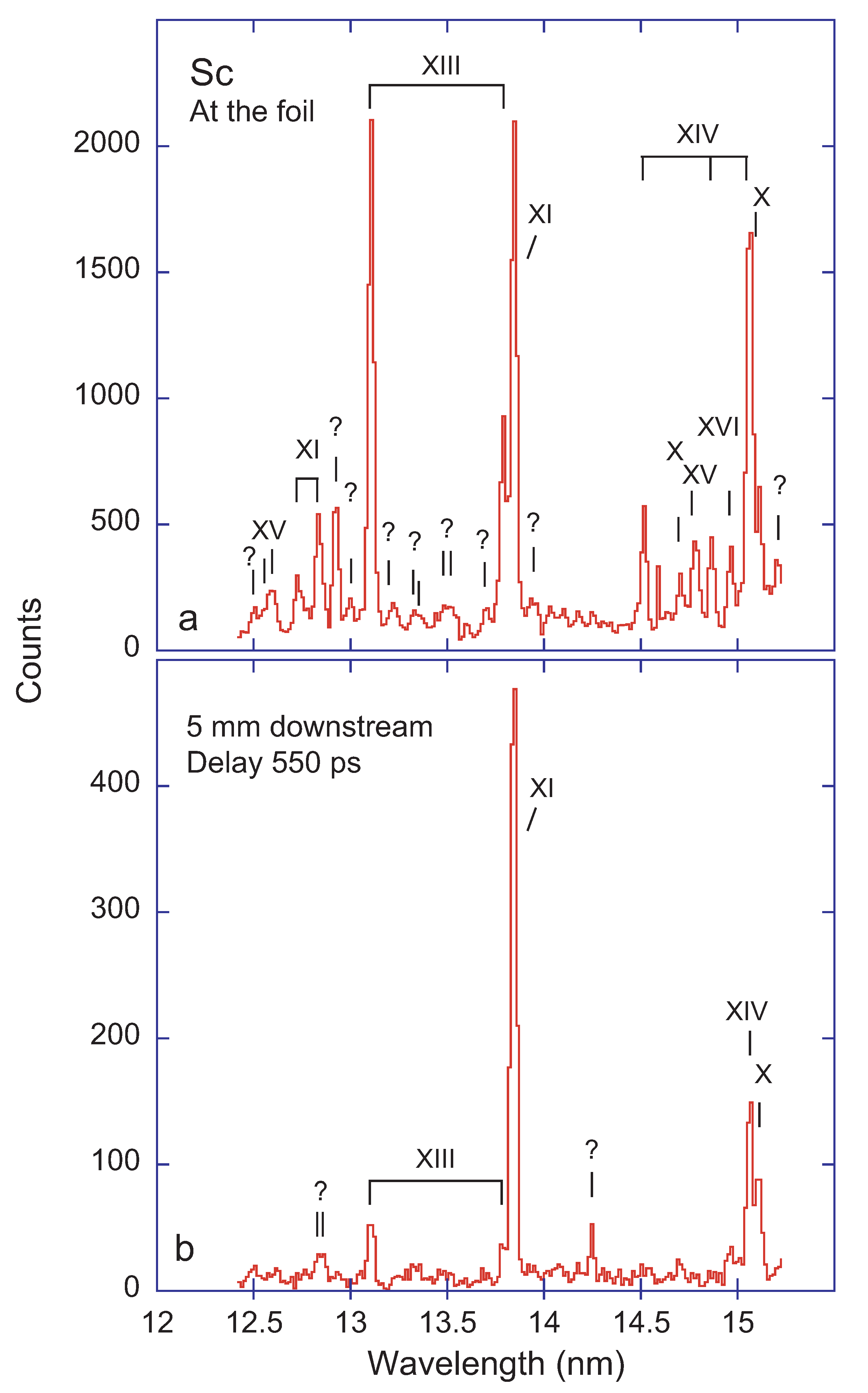
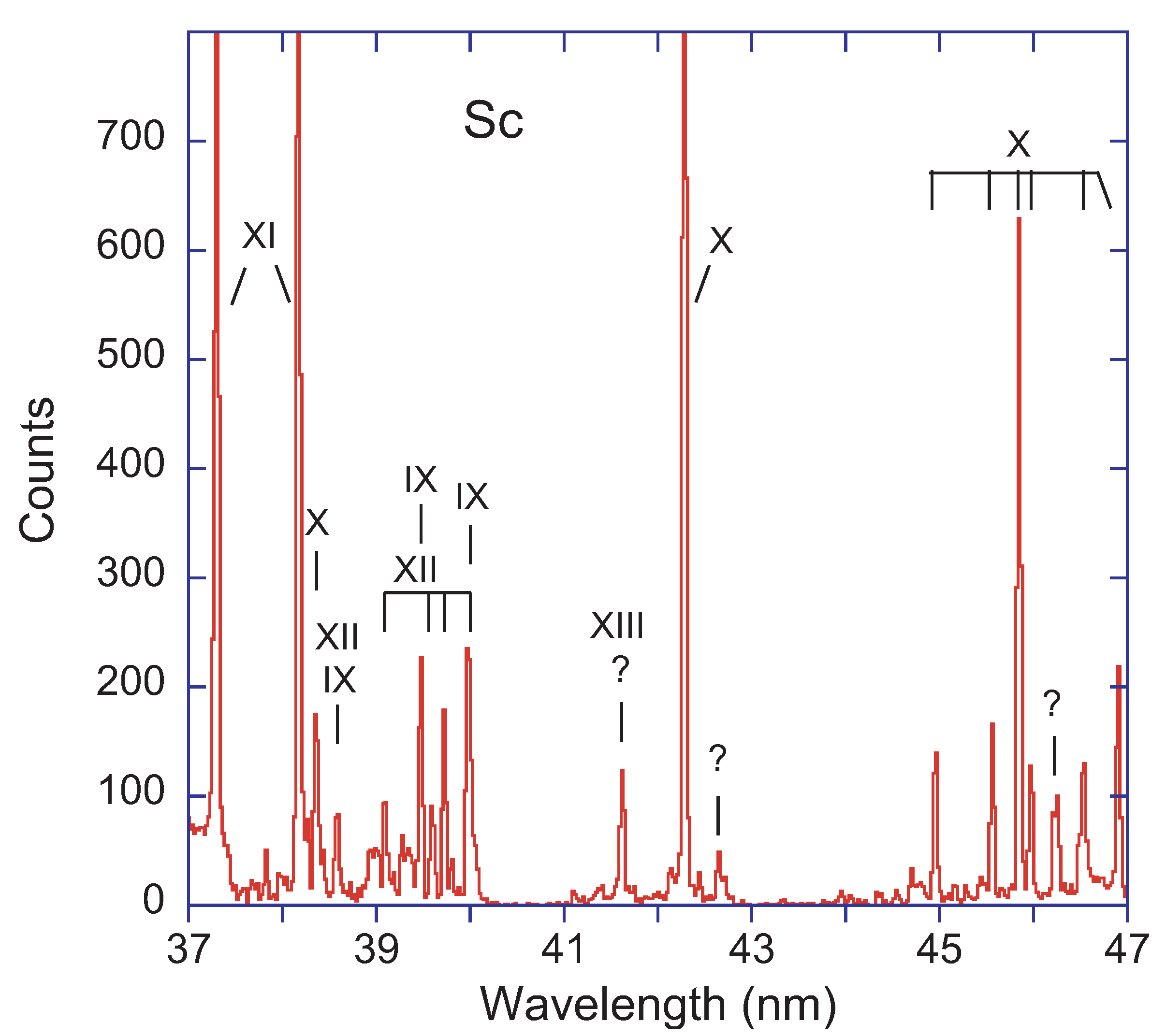
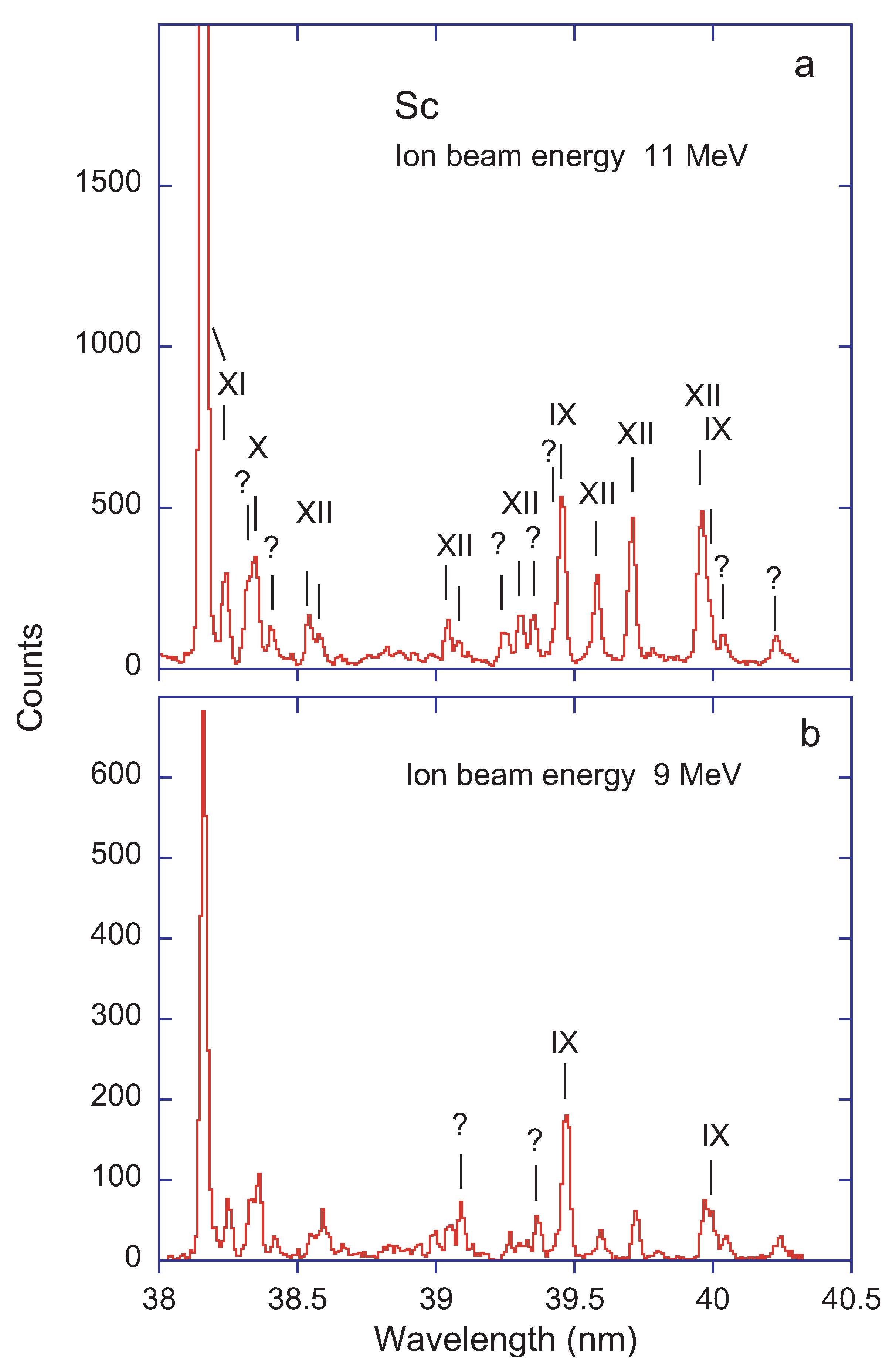
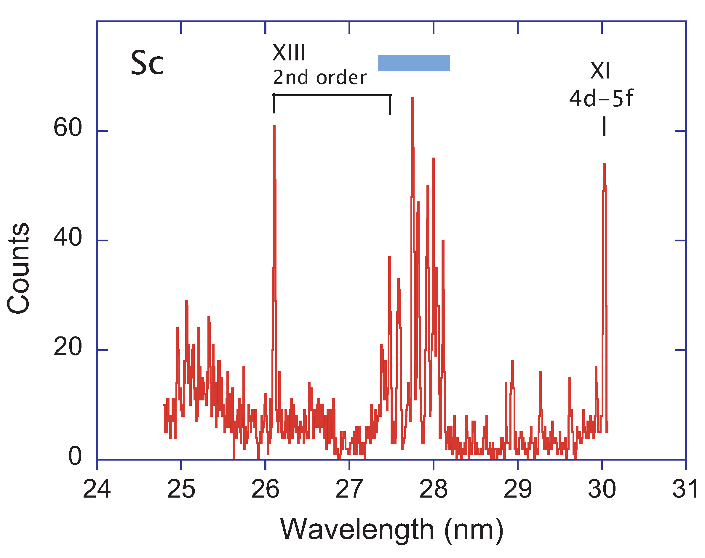
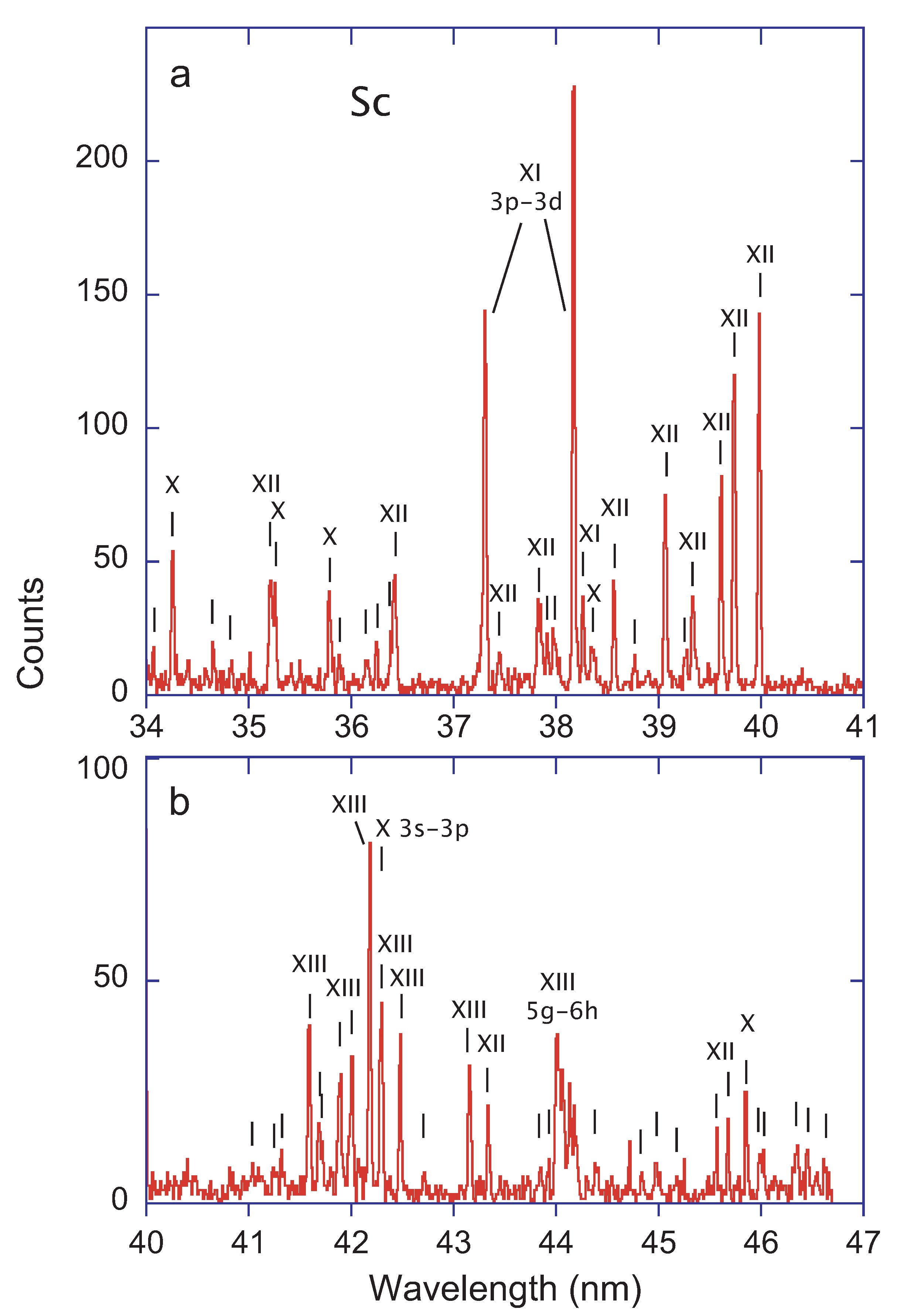
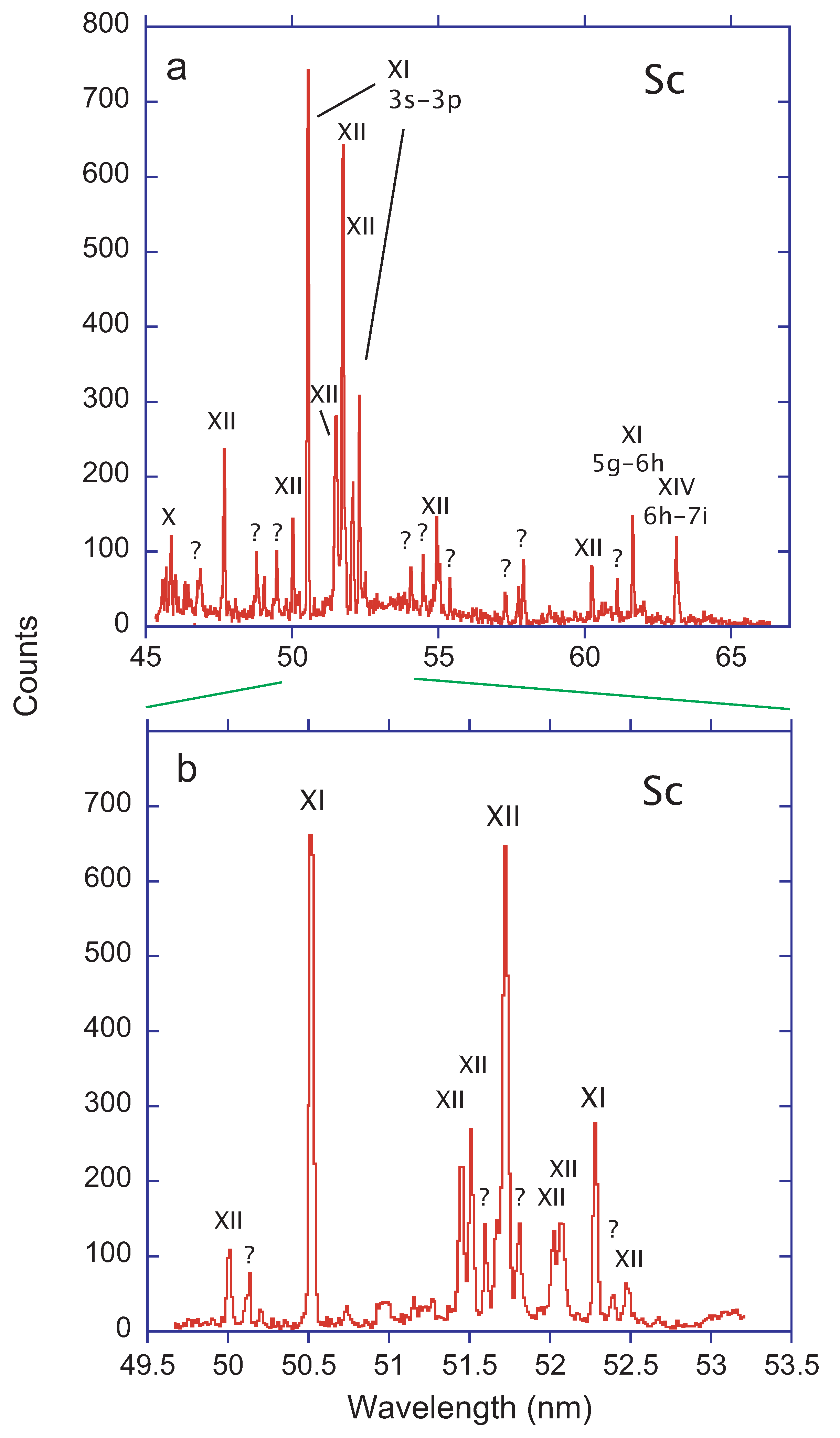
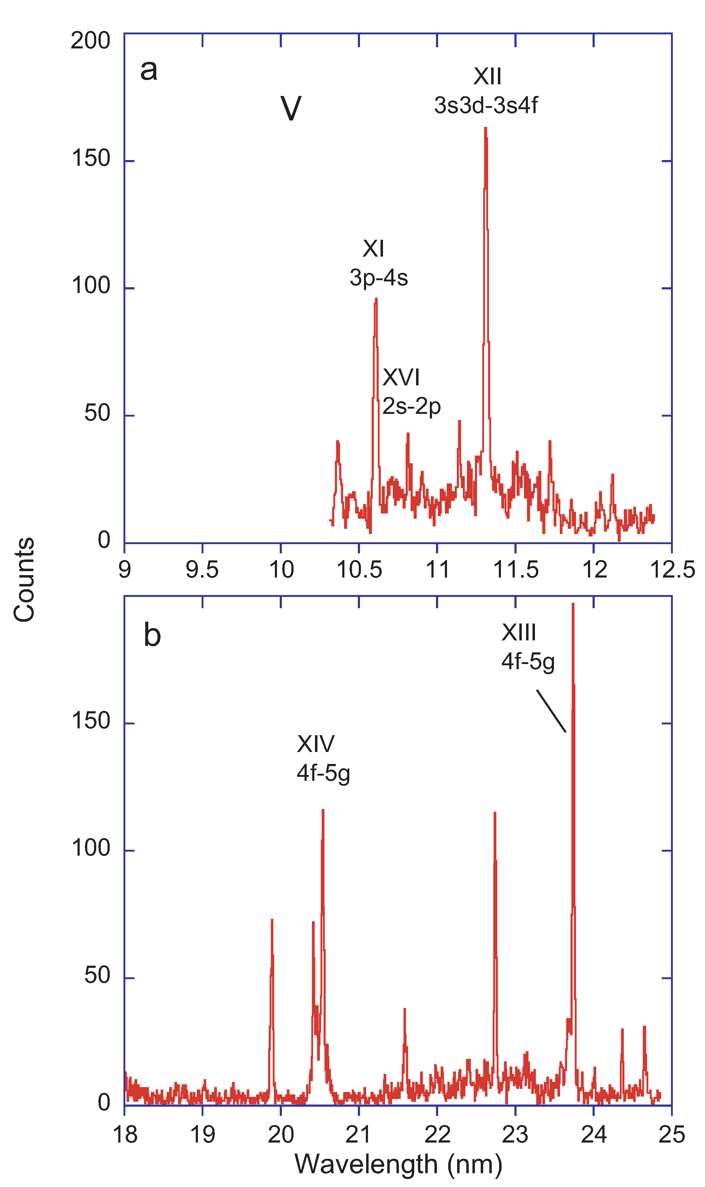
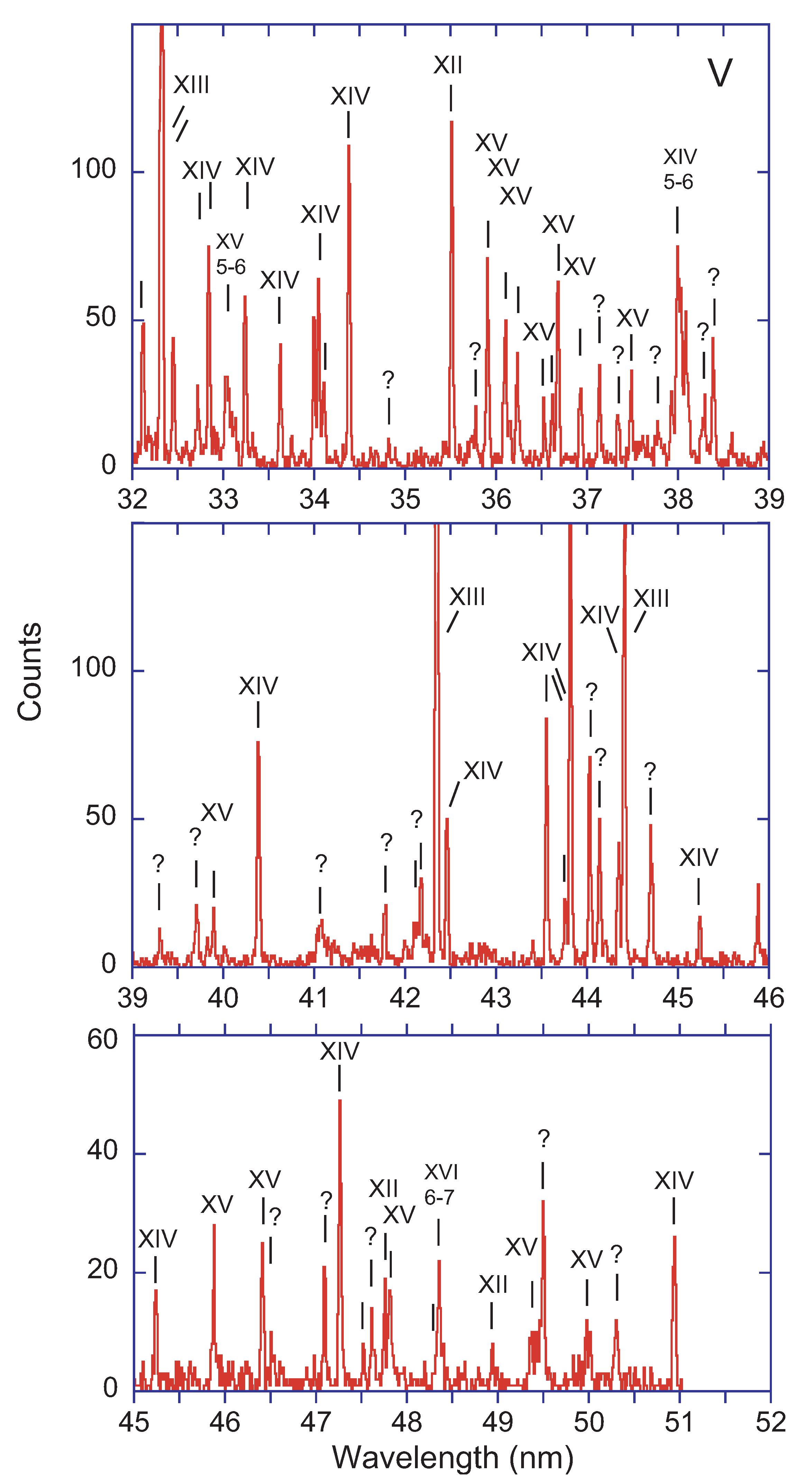
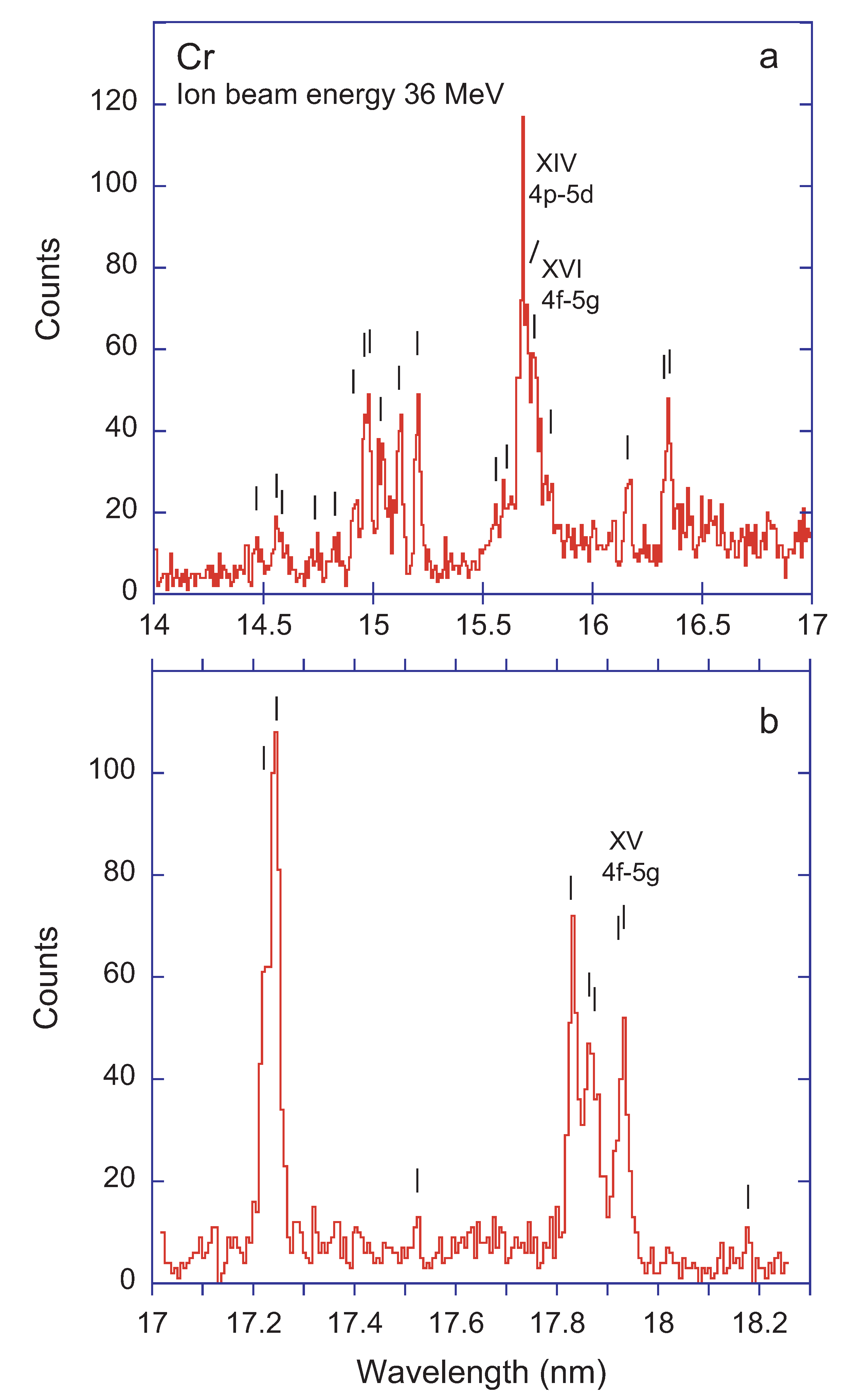
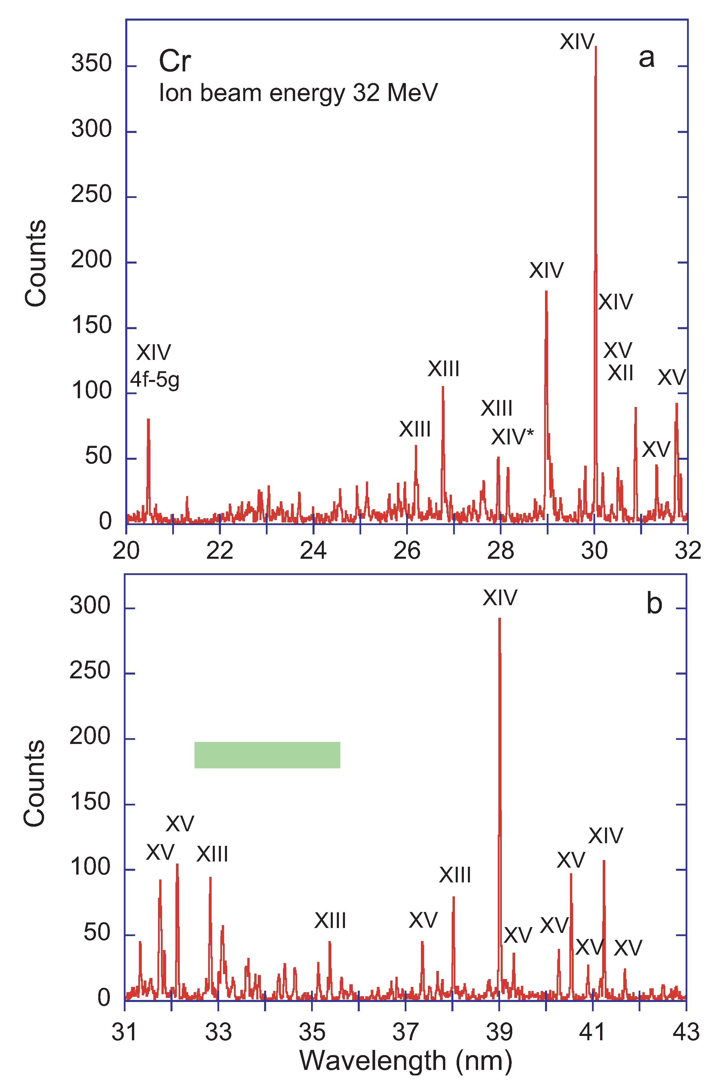
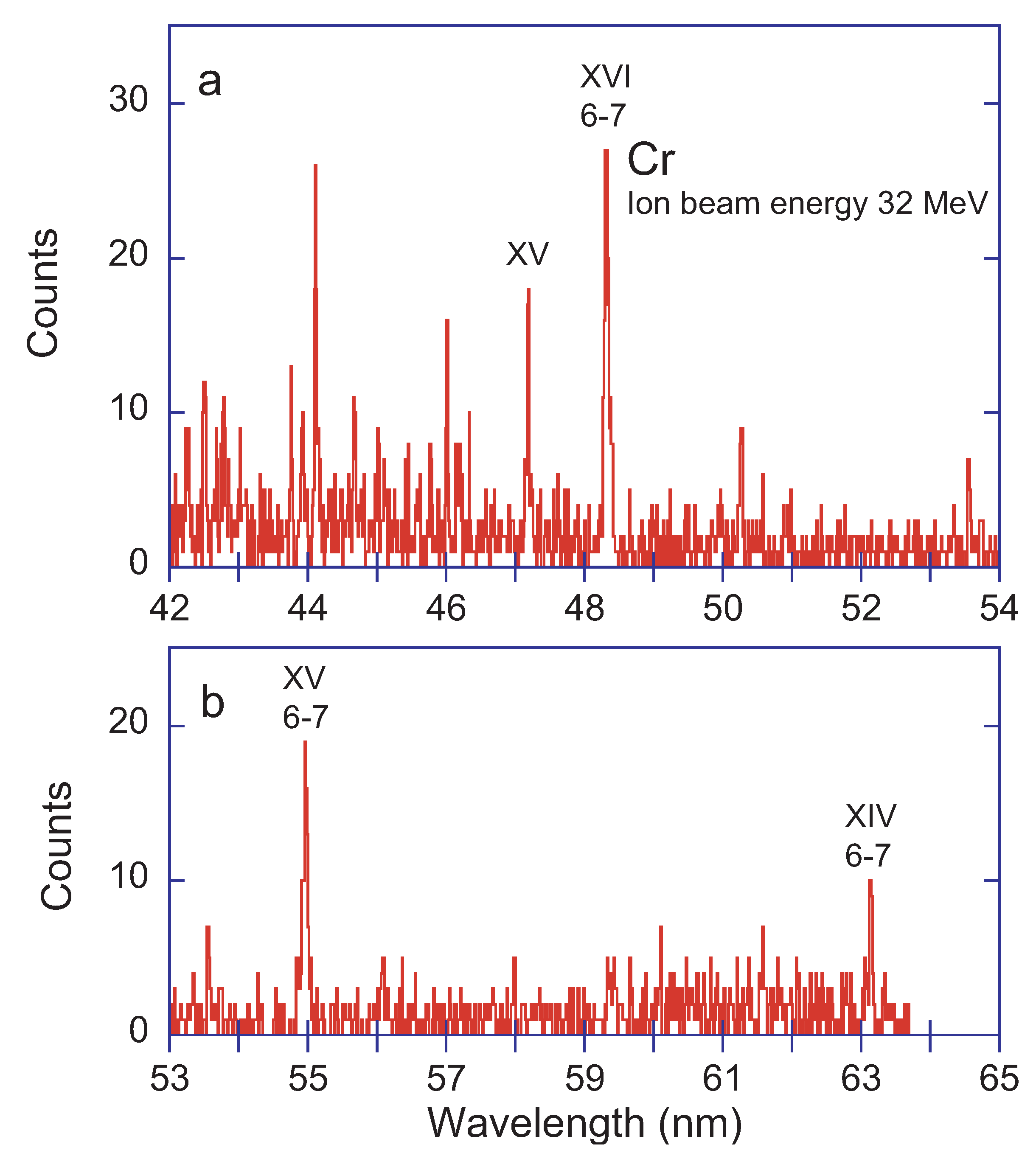
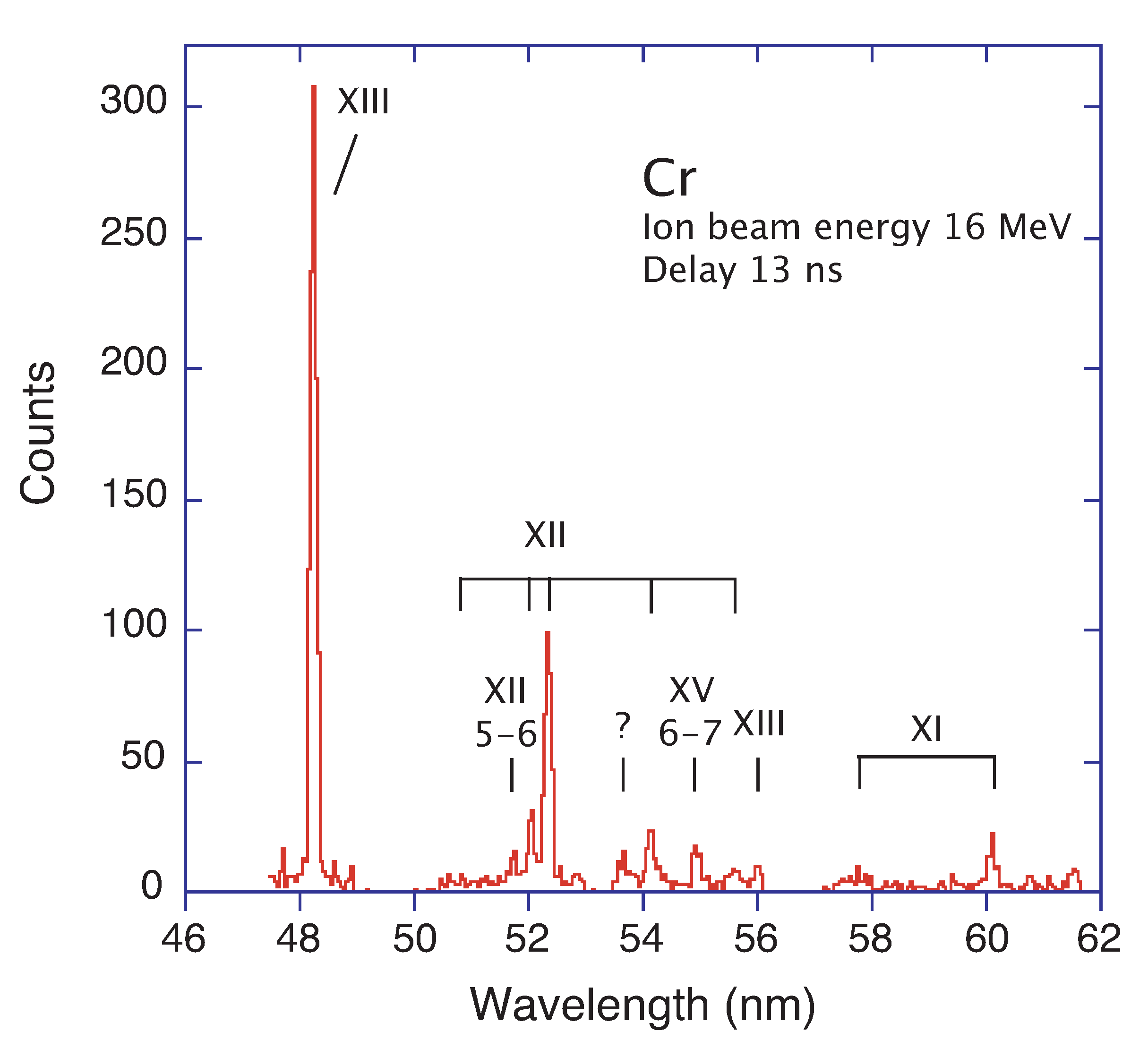
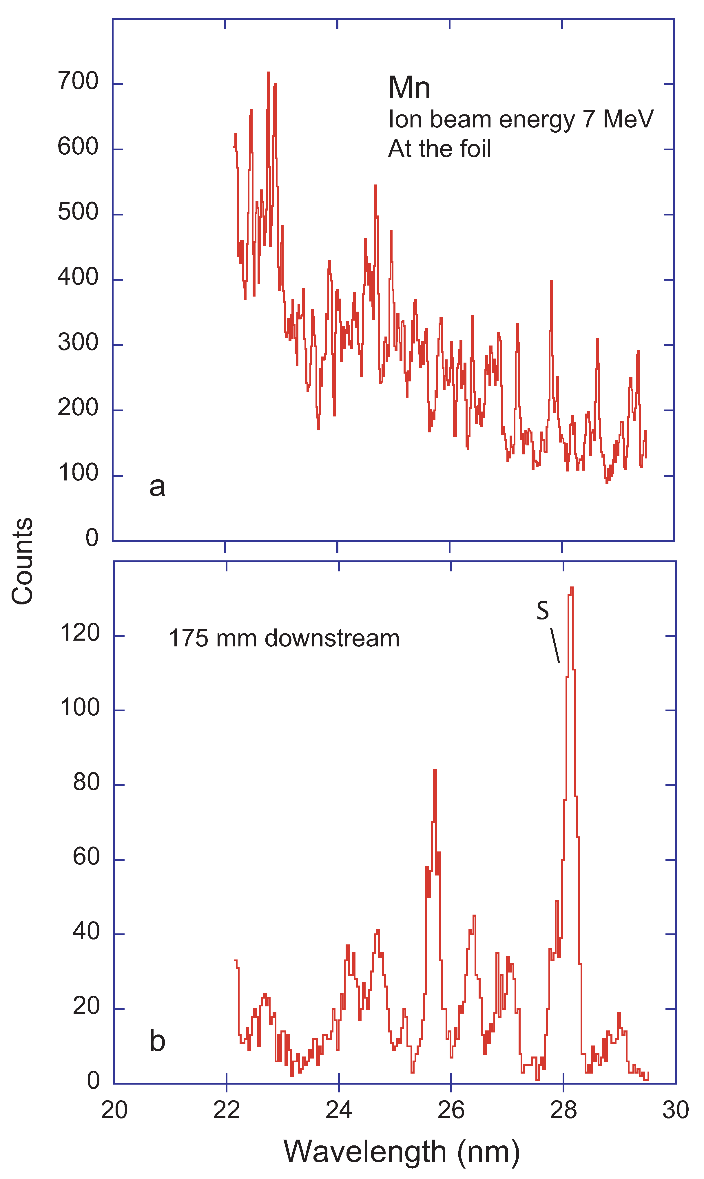
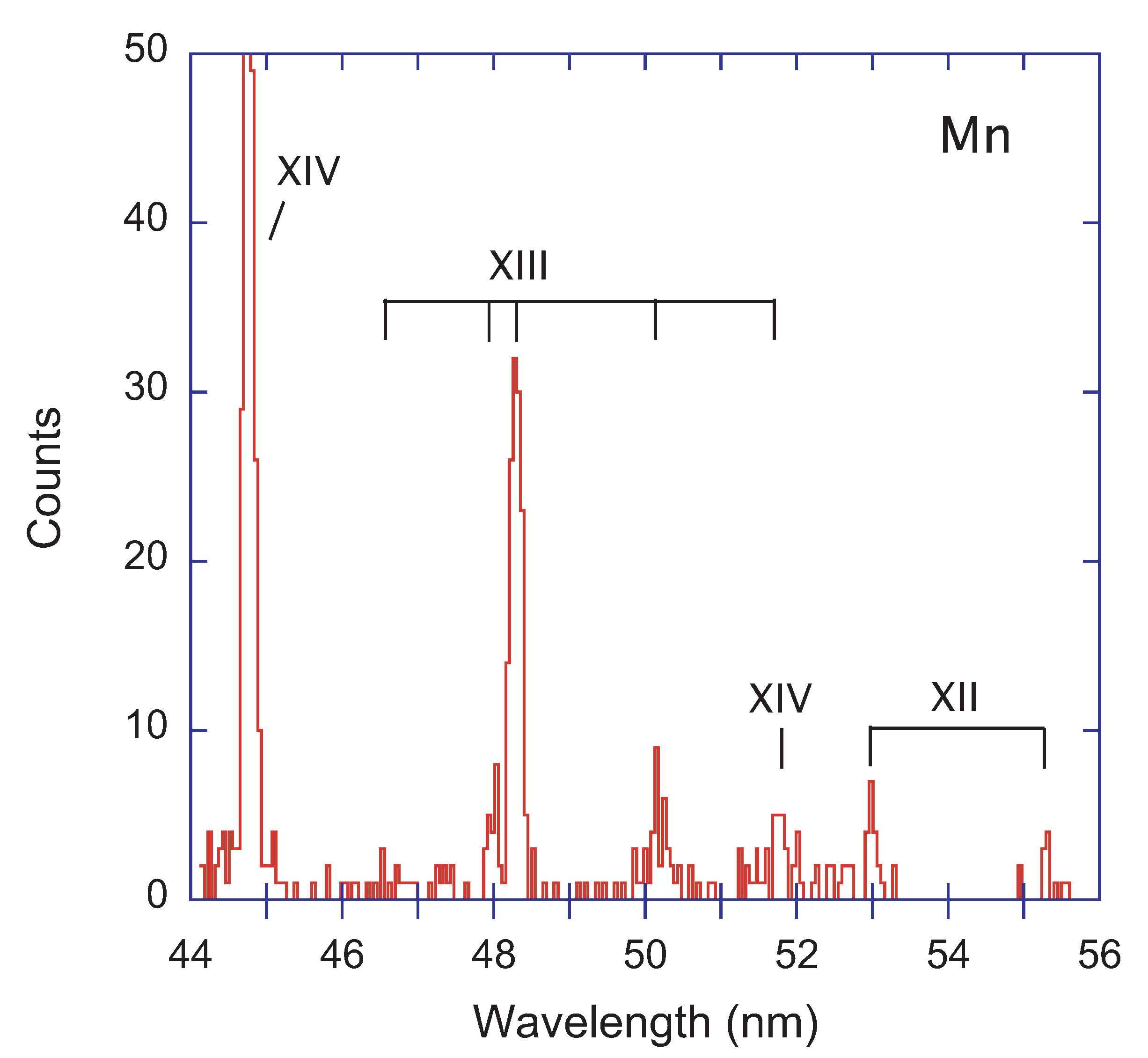
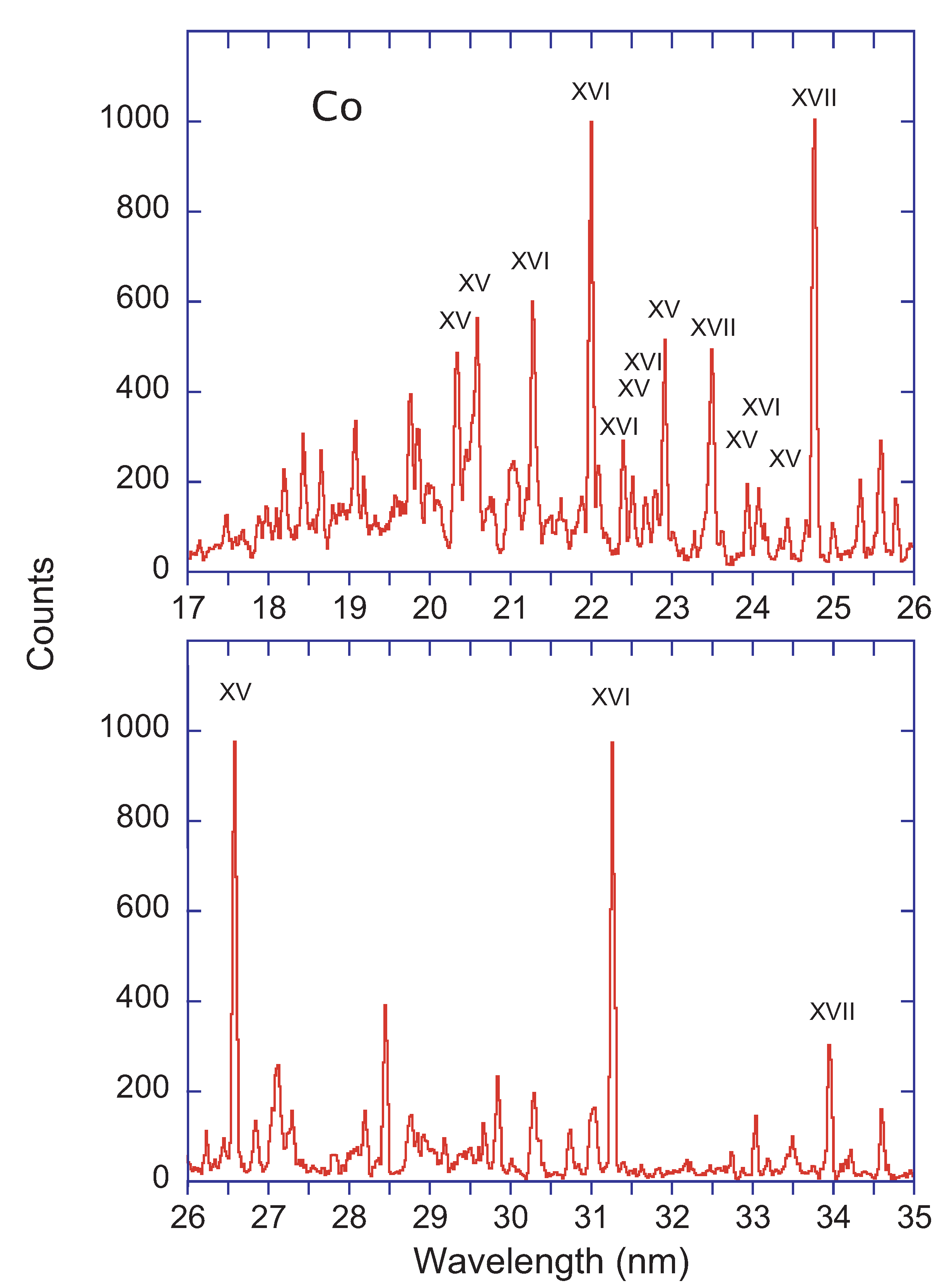
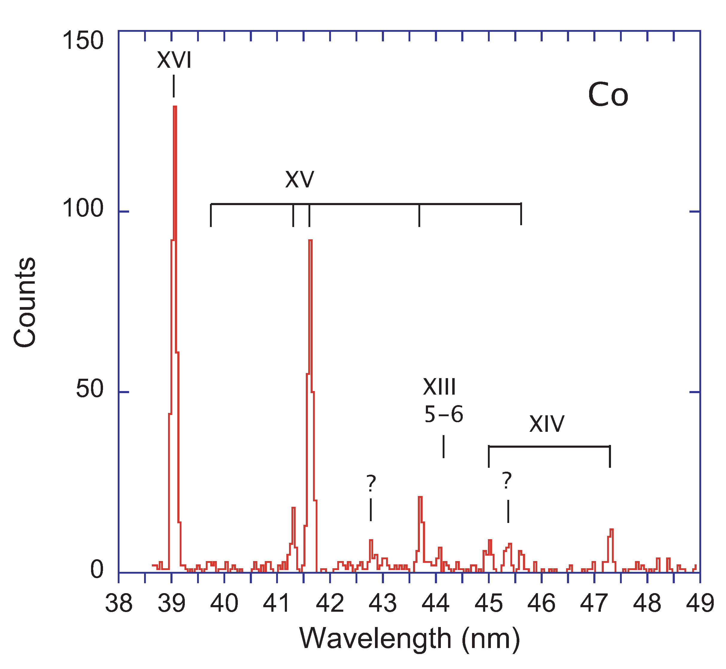
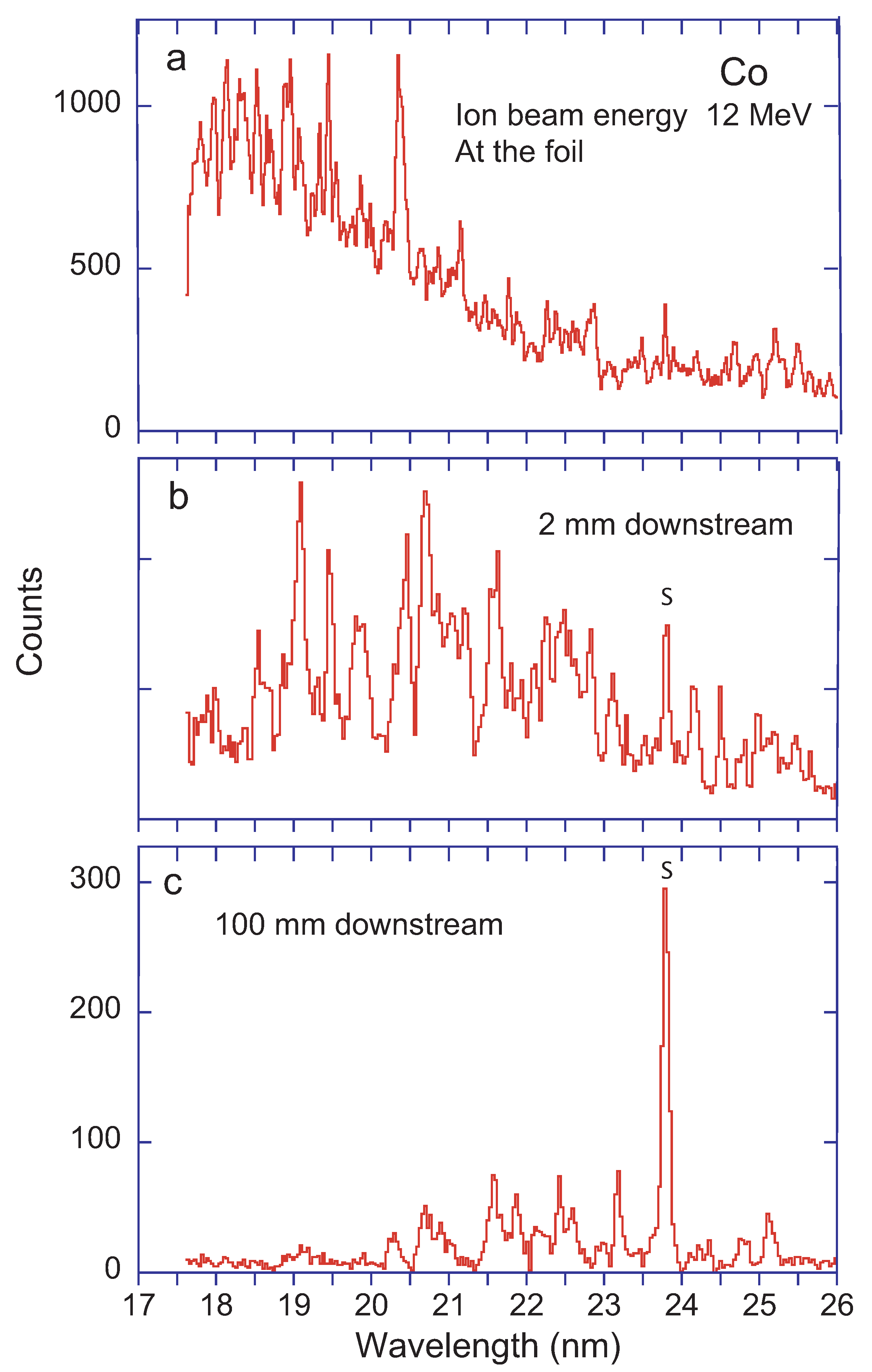
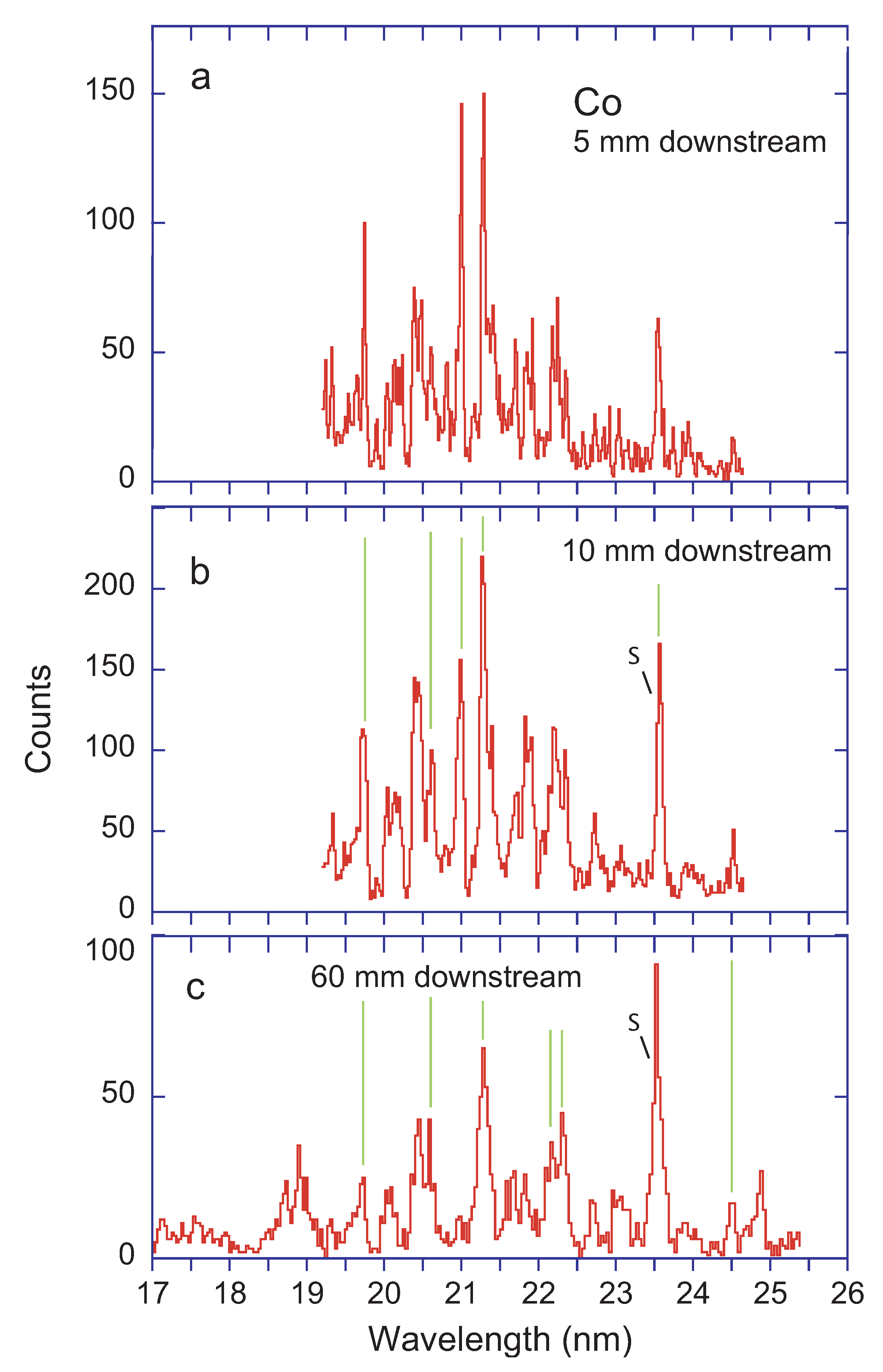
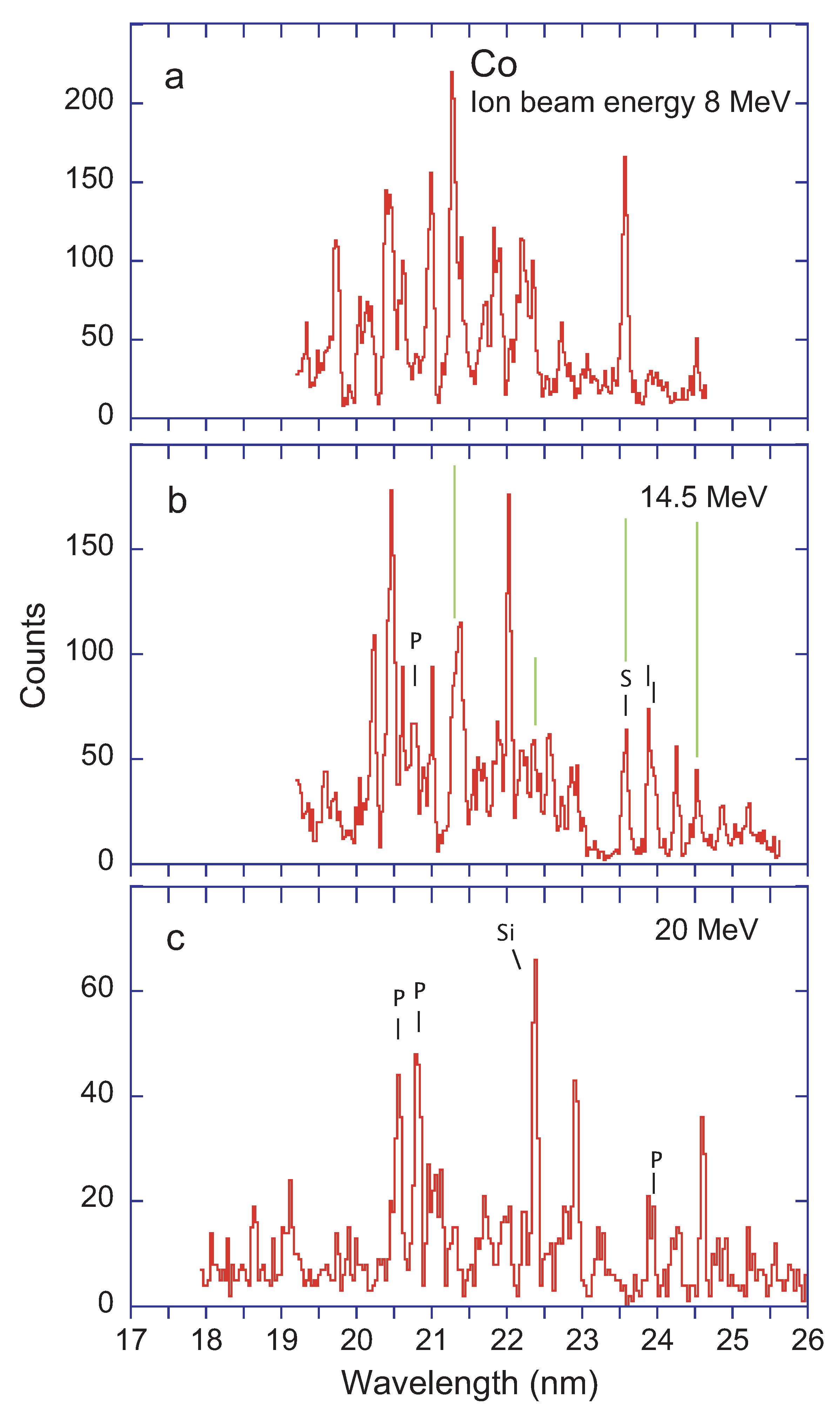
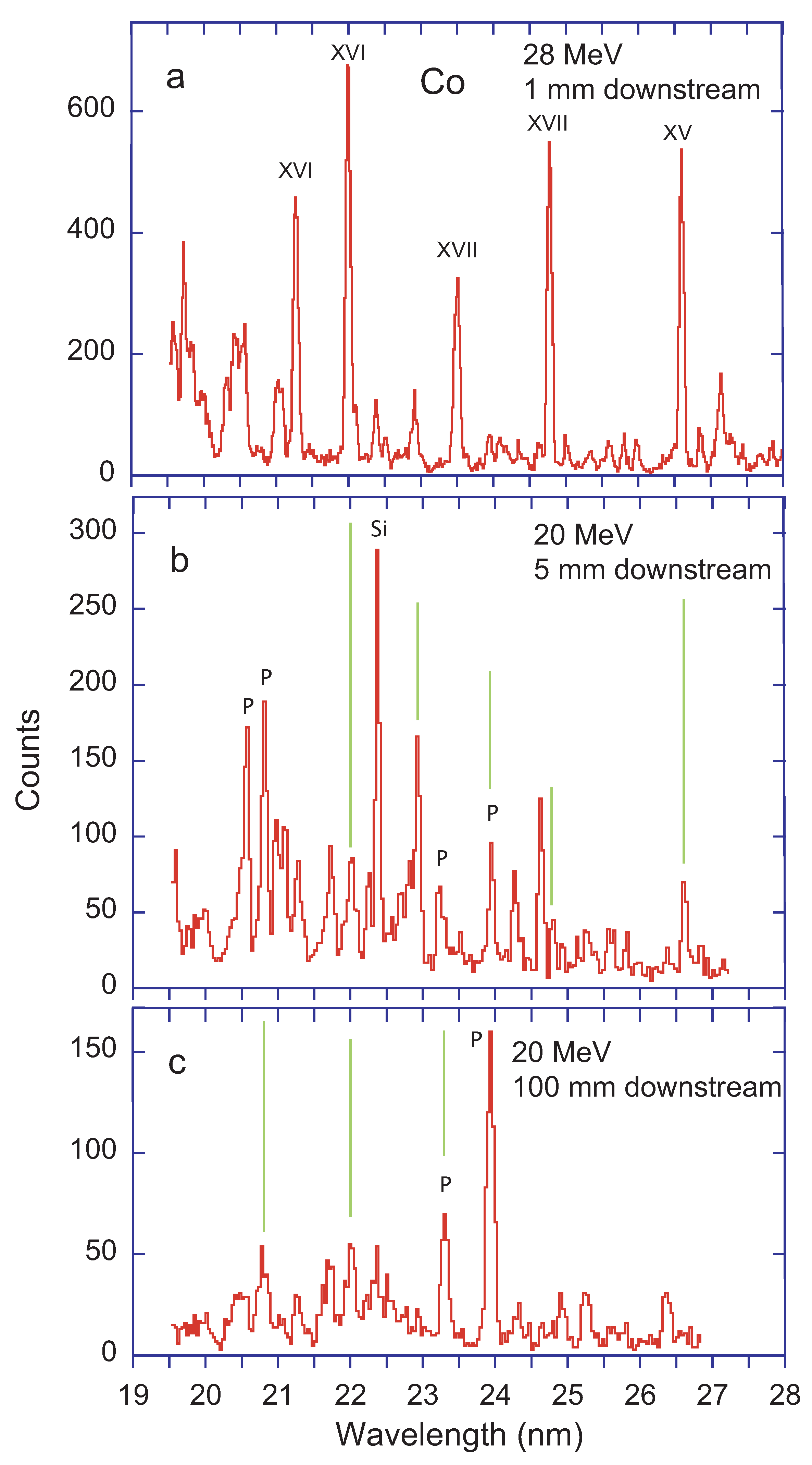
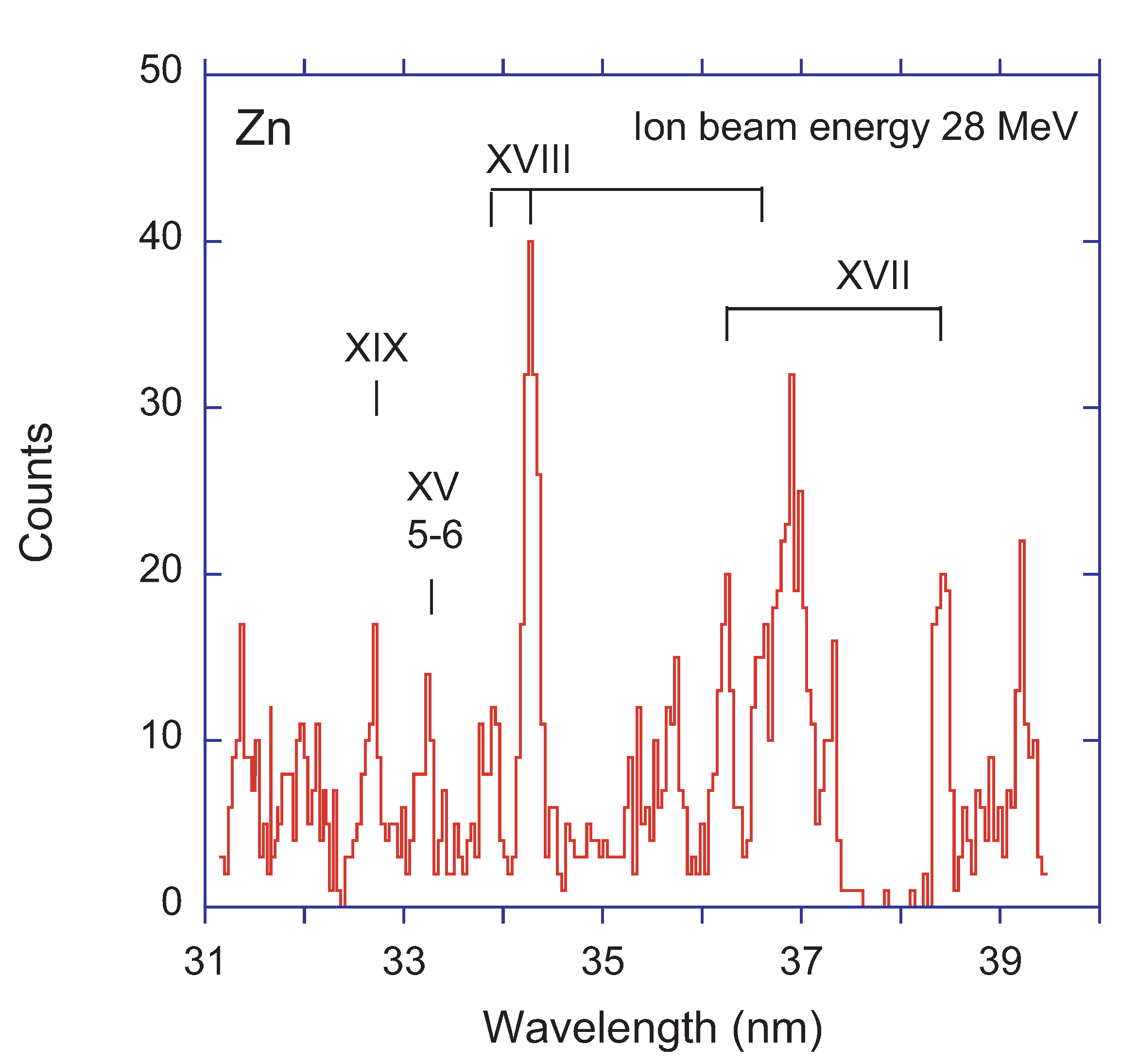
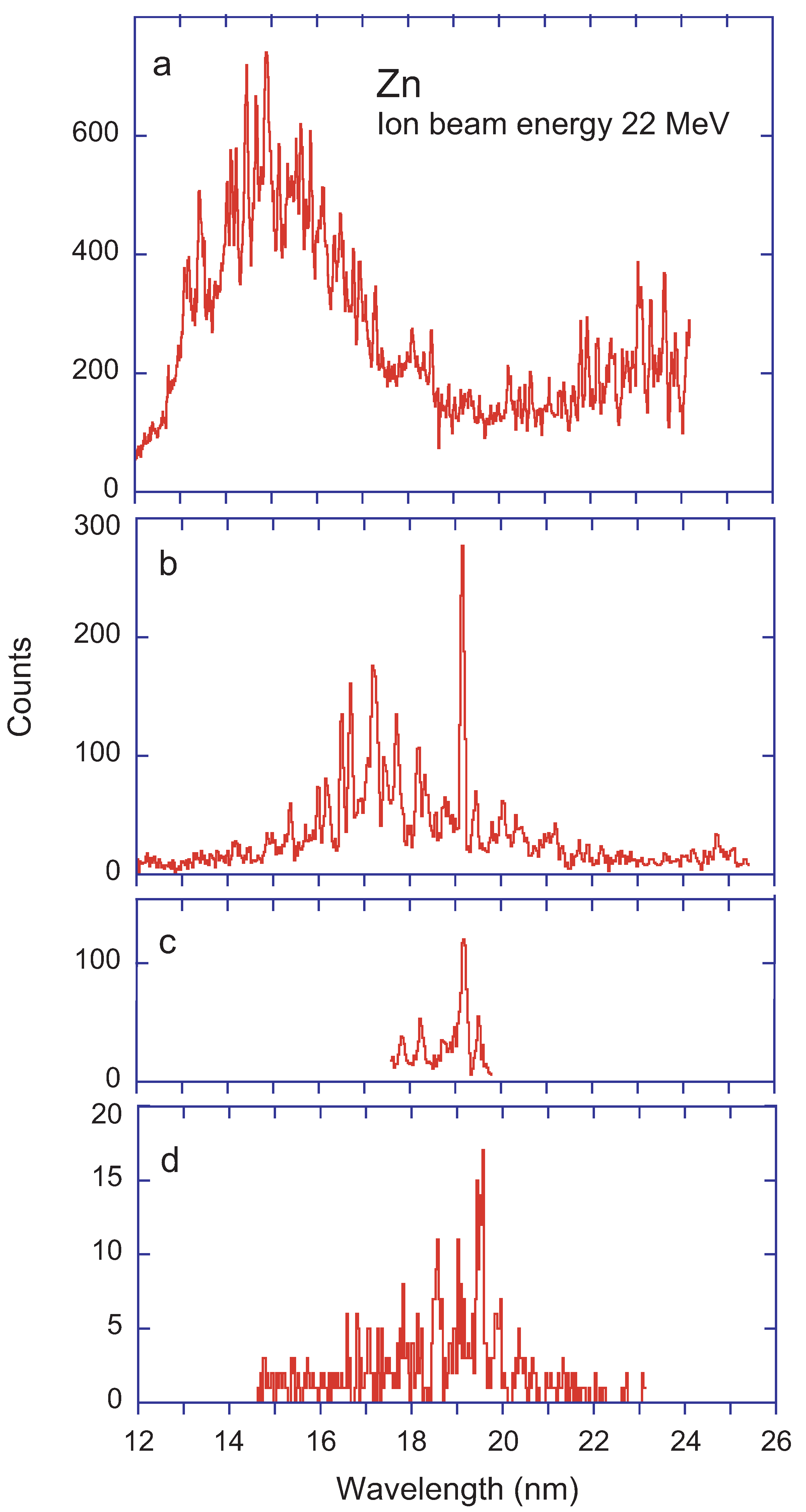
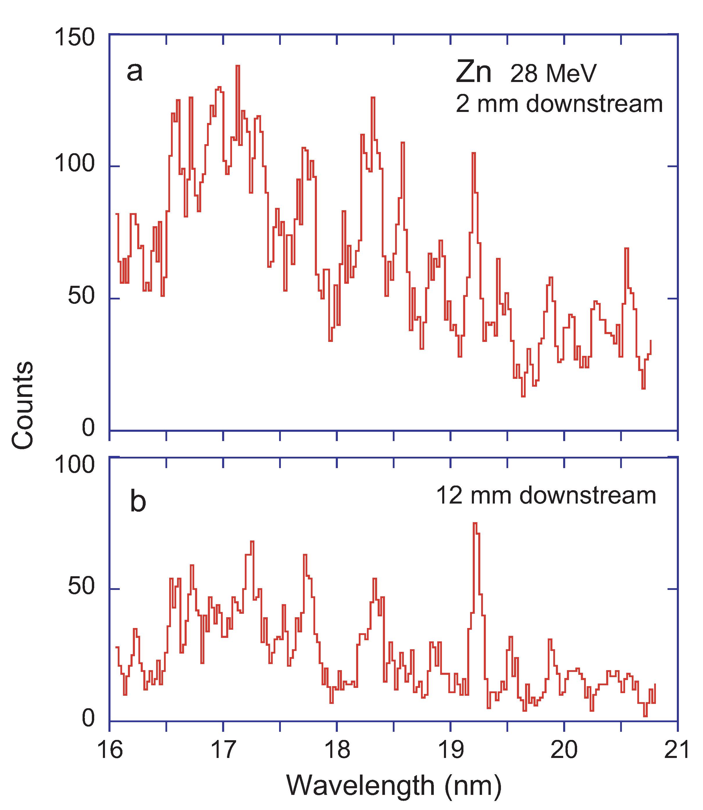
Table 1.
EUV wavelengths (in nm) of yrast transitions in hydrogenic approximation. This simple estimate uses the Bohr formula. Because of interactions of the valence electron with the electron core, the real – (with and ) transition arrays are expected on the short-wavelength side of the estimate.
Table 1.
EUV wavelengths (in nm) of yrast transitions in hydrogenic approximation. This simple estimate uses the Bohr formula. Because of interactions of the valence electron with the electron core, the real – (with and ) transition arrays are expected on the short-wavelength side of the estimate.
| Spectrum Number | 3d–4f | 4f–5g | 5g–6h | 6h–7i | 7i–8k |
|---|---|---|---|---|---|
| VI | 52.07 | 112.51 | |||
| VII | 38.26 | 82.66 | |||
| VIII | 29.29 | 63.28 | 116.50 | ||
| IX | 23.14 | 50.00 | 92.05 | ||
| X | 18.75 | 40.50 | 74.56 | 123.66 | |
| XI | 15.49 | 33.47 | 61.62 | 102.20 | |
| XII | 13.02 | 28.13 | 51.78 | 85.87 | |
| XIII | 11.09 | 23.97 | 44.12 | 73.17 | 112.74 |
| XIV | 9.56 | 20.66 | 38.04 | 63.09 | 97.21 |
| XV | 8.33 | 18.00 | 33.14 | 54.96 | 84.68 |
| XVI | 7.32 | 15.82 | 29.13 | 48.39 | 74.42 |
| XVII | 6.49 | 14.01 | 25.80 | 42.79 | 65.92 |
Table 2.
Cobalt data recorded at positions 5 mm (600 ps delay) and 100 mm (12 ns delay) downstream. Ion beam energy 20 MeV (see Figure 26). Wavelengths in nm. Wavelength uncertainty 0.01 nm (medium to strong lines) to 0.02 nm (weak lines) statistically, 0.015 nm systematically.
Table 2.
Cobalt data recorded at positions 5 mm (600 ps delay) and 100 mm (12 ns delay) downstream. Ion beam energy 20 MeV (see Figure 26). Wavelengths in nm. Wavelength uncertainty 0.01 nm (medium to strong lines) to 0.02 nm (weak lines) statistically, 0.015 nm systematically.
| Delay 600 ps | Delay 12 ns | Reference Lines [7] | |||
|---|---|---|---|---|---|
| Wavelength | Amplitude | Wavelength | Amplitude | Wavelength | Spectrum |
| 19.560 | 68 | ||||
| 19.625 | 16 | ||||
| 19.749 | 19 | ||||
| 19.859 | 33 | ||||
| 19.914 | 29 | ||||
| 19.994 | 29 | 19.969 | 8 | ||
| 20.069 | 17 | ||||
| 20.230 | 14 | ||||
| 20.337 | 16 | ||||
| 20.405 | 17 | 20.396 | 19 | ||
| 20.468 | 50 | ||||
| 20.555 | 154 | 20.521 | 20 | ||
| 20.740 | 38 | 20.744 | 29 | ||
| 20.805 | 161 | 20.827 | 22 | ||
| 20.963 | 99 | ||||
| 20.996 | 45 | 21.019 | 10 | ||
| 21.077 | 96 | ||||
| 21.182 | 13 | ||||
| 21.258 | 59 | 21.255 | 21 | ||
| 21.330 | 26 | 21.377 | 2 | ||
| 21.546 | 17 | 21.5145 | XVI | ||
| 21.626 | 18 | 21.593 | 16 | ||
| 21.707 | 36 | 21.707 | 37 | ||
| 21.733 | 43 | ||||
| 21.907 | 23 | 21.904 | 15 | ||
| 21.996 | 68 | 22.007 | 45 | 21.9915 | XVI |
| 22.071 | 24 | ||||
| 22.236 | 55 | 22.205 | 21 | ||
| 22.360 | 249 | 22.344 | 40 | ||
| 22.433 | 27 | ||||
| 22.550 | 26 | 22.522 | 27 | ||
| 22.677 | 49 | ||||
| 22.774 | 39 | 22.722 | 16 | ||
| 22.821 | 44 | ||||
| 22.917 | 154 | 22.919 | 13 | 22.9037 | XVI |
| 23.064 | 14 | ||||
| 23.208 | 53 | ||||
| 23.288 | 26 | 23.287 | 62 | ||
| 23.398 | 9 | ||||
| 23.503 | 18 | 23.4918 | XVII | ||
| 23.615 | 15 | ||||
| 23.840 | 12 | ||||
| 23.934 | 84 | 23.920 | 147 | ||
| 24.026 | 9 | ||||
| 24.131 | 11 | ||||
| 24.253 | 72 | 24.294 | 16 | ||
| 24.323 | 32 | ||||
| 24.445 | 8 | ||||
| 24.604 | 81 | ||||
| 24.634 | 47 | 24.647 | 6 | ||
| 24.758 | 38 | 24.7540 | XVII | ||
| 24.824 | 26 | ||||
| 24.911 | 20 | 24.900 | 20 | ||
| 25.000 | 15 | ||||
| 25.103 | 34 | ||||
| 25.244 | 35 | 25.238 | 26 | ||
| 25.295 | 18 | ||||
| 25.354 | 18 | ||||
| 25.544 | 27 | ||||
| 25.628 | 40 | 25.596 | 6 | ||
| 25.796 | 27 | 25.769 | 4 | ||
| 25.930 | 15 | ||||
| 25.973 | 15 | ||||
| 26.095 | 11 | ||||
| 26.208 | 16 | ||||
| 26.359 | 17 | 26.354 | 25 | ||
| 26.462 | 6 | ||||
| 26.587 | 44 | 26.5729 | XVI | ||
| 26.611 | 23 | ||||
| 26.701 | 10 | ||||
| 26.785 | 14 | ||||
| 26.821 | 20 | ||||
| 26.934 | 19 | ||||
| 27.001 | 12 | ||||
| 27.140 | 10 | ||||
Publisher’s Note: MDPI stays neutral with regard to jurisdictional claims in published maps and institutional affiliations. |
© 2021 by the author. Licensee MDPI, Basel, Switzerland. This article is an open access article distributed under the terms and conditions of the Creative Commons Attribution (CC BY) license (http://creativecommons.org/licenses/by/4.0/).
Share and Cite
MDPI and ACS Style
Träbert, E. EUV Beam-Foil Spectra of Scandium, Vanadium, Chromium, Manganese, Cobalt, and Zinc. Atoms 2021, 9, 23. https://0-doi-org.brum.beds.ac.uk/10.3390/atoms9020023
AMA Style
Träbert E. EUV Beam-Foil Spectra of Scandium, Vanadium, Chromium, Manganese, Cobalt, and Zinc. Atoms. 2021; 9(2):23. https://0-doi-org.brum.beds.ac.uk/10.3390/atoms9020023
Chicago/Turabian StyleTräbert, Elmar. 2021. "EUV Beam-Foil Spectra of Scandium, Vanadium, Chromium, Manganese, Cobalt, and Zinc" Atoms 9, no. 2: 23. https://0-doi-org.brum.beds.ac.uk/10.3390/atoms9020023
Note that from the first issue of 2016, this journal uses article numbers instead of page numbers. See further details here.