Relativistic Coupled-Cluster Calculations of Isotope Shifts for the Low-Lying States of Ca II in the Finite-Field Approach


1
Institut de Physique de Nice, Université Côte d’Azur, CNRS, 06108 Nice, France
2
Atomic, Molecular and Optical Physics Division, Physical Research Laboratory, Navrangpura, Ahmedabad 380009, India
*
Author to whom correspondence should be addressed.
†
These authors contributed equally to this work.
Atoms 2021, 9(2), 26; https://0-doi-org.brum.beds.ac.uk/10.3390/atoms9020026
Submission received: 17 February 2021
/
Revised: 24 April 2021
/
Accepted: 27 April 2021
/
Published: 3 May 2021
(This article belongs to the Section Atomic, Molecular and Nuclear Spectroscopy and Collisions)
Abstract
:We have evaluated the isotope shift (IS) constants of the first five low-lying fine-structure states of the singly charged calcium ion (Ca II) by adopting a finite-field (FF) approach in the relativistic coupled-cluster (RCC), a method developed by us and by using a code also developed by us. A similar previous calculation using singles and doubles approximation RCC theory (RCCSD method), gives results for the individual states in the FF approach that deviate substantially, while the differential values (the shifts of the spectral lines) agree reasonably well with other theoretical results and with experiments. However, we find a contrasting trend from the FF approach using our RCCSD method although calculations with the Dirac–Hartree–Fock (DHF) method shows good agreement. Our results also show that inclusion of partial triple excitations in the perturbative approach (RCCSD(T) method) through energy derivation lessens accuracy, but these results can be improved when triple excitations are included in the wave function that determines the RCC equations. The differences between the RCCSD and RCCSD(T) results demonstrate the importance of triple excitations in evaluating energies and IS constants for Ca II. Finally, we also present ab initio values of IS’s between the S–P, S–D, and D–P transitions in the DHF, and RCCSD and RCCSD(T) approximations and this is compared to the previously reported values (theoretical as well as experimental).
1. Introduction
The study of the atomic isotope shift (IS) can provide seminal information in the intersection between nuclear and atomic physics [1]. Accurate data, experimental and theoretical, on IS can be used to extract fundamental properties such as the nuclear mean square radius [2] and information about the existence of new particles [3]. Within a single species, the variation of the isotope shift with a neutron number gives insight into the nuclear shell structure and nucleon-nucleon interaction [4]. Deriving nuclear properties from atomic spectra provides an important complement to direct measurements of the nucleus, as the lower energies involved allows excellent resolutions. From an atomic viewpoint, precise spectroscopic data has astrophysical significance [5], such as in analyses of stellar abundances. Metrological applications are also often acutely dependent on atomic data.
The electronic configuration of singly ionised calcium (Ca II), iso-electronic with neutral potassium (K I), is well known, but nuclear effects on the spectrum is still an active area of research—especially for radioactive isotopes. Important experimental studies were reported on in, for example [3,6,7,8,9,10]. Such work is complemented by theoretical investigations, see [11,12,13,14], and together they contribute to the understanding of, for example, nuclear structure and relativistic effects. Comparisons between theoretical and empirical data also constitute critical tests of relativistic many-body quantum mechanical computational methods. The latter can be made particularly accurate in K-like systems, due to the single valence electron and the intermediate mass. The Ca isotopes provide a sensitive test of nuclear structure theory, with one of its isotopes having a doubly-magic composition of nucleons [4].
There are three main contributions to the overall isotope shift (see for example [15] or [16]), occurring from the differences in spatial charge distribution (the field shift—FS) and in nuclear mass (the mass shift). The latter is, in turn, split up into one component arising from a mass polarisation effect in the centre-of-mass referential (the specific mass shift—SMS) and another one which is the difference in the reduced mass between different isotopes (the normal mass shift—NMS). The mass specific components typically dominate for reasonably light, or intermediate nuclei.
For the theoretical determination of IS, isotope independent parameters should be evaluated and the respective isotope dependent quantities should then be multiplied to them for obtaining the final shifts. Therefore, accurate calculations of the FS, NMS, and SMS constants are the essential theoretical interest. This requires employing a reliable many-body method for the evaluation of the IS constants. Coupled-cluster (CC) theory in the relativistic framework (RCC) is today considered the gold standard among the available many-body methods for the accurate determination of atomic properties [17,18,19,20]. A truncated (R)CC method not only accounts for different physical effects due to the electron correlation effects to all-orders, it also satisfies the size-extensitivity and size-consistent characteristics of the many-body theory.
For a given many-body theory, there are different procedures available to determine the first-order properties. For example, it is possible to evaluate the IS constants in the direct expectation value evaluation approach, or alternatively to estimate them by adopting finite-field (FF) procedures [21]. An alternative route is to adopt more intriquate approaches, such as considering the bi-orthogonal wave function and analytical gradient approaches [18]. Since the operators that describe the IS are scalar operators (see Section 2), the FF procedure is often used to determine the IS constants.
In this work, we employ the RCC theory in the FF approach to evaluate the FS, NMS, and SMS constants of Ca II. This will serve two purposes. First, an earlier calculation using the singles and doubles approximation in the RCC theory (RCCSD method), and the FF approach, showed a significant discrepancy between the results for individual states from the RCC theory and older calculations based on other methods [14]. Our analysis facilitates addressing this ambiguity. Second, the NMS constants are often estimated using the scaling relation of kinetic energy with the total energy of the virial theorem. Improved ab initio results for NMS constants will also address this. We report results for the first five low-lying states of Ca II, and the transitions involving them. Study of isotope shifts in these particular transitions are of pronounced interest for probing nuclear structure and for searching for the existence of new bosonic particles [3].
2. Theoretical Method
2.1. Theory of IS in Atomic Systems
The IS of an energy level, , between an isotope, A, with mass, , and an isotope, , with mass, , is given by a product of nuclear and atomic factors as:
where is the field-shift (FS) constant, and with the difference between the nuclear mean-square charge radii of the two isotopes. is the mass-shift (MS) constant. This is further divided into . It is also worth mentioning here that Equation (1) corresponds only to the first-order IS correction and higher-order effects are neglected in the present analysis. Within a reasonably good approximation, determinations of , , and are assumed to be independent of isotope, but dependent on the atomic wave functions. Therefore, it is imperative to evaluate the atomic wave functions accurately in order to reliably determine the IS constants.
It should be added that the evaluation of atomic wave functions also depends on the finite-size of the nucleus, and the latter can be determined for a given isotope. Therefore, we consider the isotope Ca when we determine the atomic wave functions. This may result in slight differences in the evaluation of constants for different isotopes. However, this will not make any significant differences in the estimation of the ISs.
2.2. General Features of RCC Theory for One-Valence Systems
The ground state of the Ca II ion has a closed-shell core and a valence orbital in the 4s shell. Its low-lying excited states possesses the same core, but the 4s valence orbital is replaced by, for instance, the 3d or the 4p orbital. The wave functions of these low-lying states of Ca II can be calculated in the RCC theory framework by (for example, see [22,23,24] and references therein):
where is a mean-field wave function treated as reference state, and T and are the excitation operators that take care of the electron correlations among the core and valence orbitals, respectively, due to the neglected residual interactions in the determination of . Owing to the fact that all the investigated states of Ca II in this work have a common core, we define for computational convenience the reference state as for the Dirac–Hartree–Fock (DHF) wave function of the closed-core. From the Schrödinger equation , with the atomic Hamiltonian H and energy eigenvalue of the corresponding state, the T and amplitude solving equations are given by [22,23,24]:
respectively, where the superscript * over the reference states indicates that they refer to the excited determinants with respect to the respective reference states. The subscript N indicates that the operators are in the normal order form, and with subscript l denotes linked terms. The energies of the closed-shell (), and of the closed-shell with the valence orbital configurations, are obtained from [22,23,24]:
Since Equation (3) depends on , both Equations (3) and (4) are solved simultaneously. In addition, and are not the actual physical observables, so to validate the calculation of the wave function we evaluate the electron affinity of an electron with the valence orbital v (equivalent to the ionisation potential of the corresponding orbital) and compare this with the experimental value. Since the objective of the present work is to verify the IS results from the FF approach, we consider only the single and double excitations through the RCC operators (known as the RCCSD method approximation) by defining:
We also include leading-order contributions from the valence triple excitations, (referred to as RCCSD(T) calculations) by defining a perturbative RCC operator as:
where and are the indices of the occupied and unoccupied orbitals, respectively, and the ’s are their corresponding single particle orbital energies. For computational simplicity, we include contributions from through the energy equation only in Equation (4). However, it is expected that the electron correlation contributions from this operator can have large cancellations when it is included in both Equations (3) and (4) simultaneously. Thus, the differences in the results between the RCCSD and RCCSD(T) methods will only indicate the typical order of contributions from the valence triple excitations in the considered Ca II ion.
2.3. FF Approach and IS Constants
The expectation value of an operator O can be determined in the FF approach by using an effective Hamiltonian , where is the atomic Hamiltonian and is a small arbitrary parameter and chosen to be in these calculations. The energy (or say the electron affinity) obtained by considering the above Hamiltonian will depend on and can be expressed as:
where superscripts (0), (1), etc. denote the order of perturbation and indicates corrections higher than the first-order. For a very small value of , we get:
Therefore, the first-order energy correction can be estimated from the above expression as:
In the perturbative approach, we have , if O is considered as the the interaction operator. Thus, Equation (9) offers the expectation value of the operator O in the FF approach.
In the present work, we use a Dirac–Coulomb atomic Hamiltonian in the calculation, given in atomic units (a.u.) by:
where and are the Dirac matrices, summations are respectively taken over electrons i and pairs of electrons in the atom, c is the speed of light, the momentum operator for electron i, the potential due to the atomic nucleus, and is the Coulomb operator. Here, is evaluated by assuming a spherically-symmetric Fermi nuclear charge distribution.
The FS, NMS, and SMS constants in Equation (1) of an atomic state can be determined as the expectation value of the respective operators as , , and . In the present calculations, we have defined these as:
where is the fine-structure constant and Z is the atomic number of the atomic system.
2.4. Generation of Single Particle Orbitals
In the relativistic theory, the single particle wave function is given by:
where and are known as the large and small components of the Dirac wave function, and represents the angular component with relativistic quantum number and projection of the angular momentum m. The radial functions are constructed as a linear combinations of known functions, , by defining them as:
and
where is the number of functions for a given l-symmetry orbital, the ’s are the unknown coefficients determined by diagonalising the matrix, and the superscripts L/S denote the large/small components.
We have used Gaussian type orbitals, GTOs, defined as:
and
where are the normalisation constants, and the optimised GTO parameters for a given orbital, and the relation between and in Equation (18) implies the kinetic balance condition.
We have considered 40 GTOs, and universal basis functions with and for each symmetry up to . Numerical radial integration are carried out on a non-linear grid distribution, with the number of grids , by defining radial distance as:
where is a very small parameter and h is the step size. In our calculation, we have used and to perform the numerical calculations. In the RCC calculations, we only allow orbitals having principal quantum number up to 20 to participate in the electron excitation processes, due to the correlation effects.
3. Results and Discussion
As an initial test of the unperturbed wave functions, we calculate the electron affinity from Equation (4) and compare the results with experimental values. The results are presented in Table 1.
The RCC calculations agrees very well with the experimentally determined data (between 0.05% and 0.5% for RCCSD), whereas the DHF data, as expected, underestimates the electron affinity (by about 3% to 11%). RCCSD(T) values are consistently lower than the RCCSD ones, demonstrating the importance of the inclusion of triple excitation for a still improved calculation of the atomic wave functions by including triple excitations through the amplitude determining equation of the RCC excitation operators.
The contributions to the overall isotope shifts were calculated, using the techniques described in Section 2, using the unperturbed wave functions with the FF contributions to the IS components, as in Equations (11)–(13), for all fine-structure levels belonging to the 4s, 3d, and 4p configurations of Ca II. The primary data are presented in Table 2. The respective pre-factors for the field shift (FS), the normal mass shift (NMS), and the specific mass shift (SMS) are shown, as calculated with three different numerical methods. Our results are compared to ones reported by Roy et al. [14] and Safronova et al. [12] when applicable. As can be seen, our FF results for the SMS constants of the individual state differ substantially from the FF values reported in [14] although the same RCC theory is employed in both the works. However, our results agree reasonably well with the calculations in [12], which are obtained using the expectation value (EV) approach in a third-order relativistic many-body perturbation theory (RMBPT).
Another observation is that the DHF values derived by the FF and EV approaches are different, owing to the fact that the FF option includes the orbital relaxation effects that can arise through the random phase approximation (RPA) in the EV approach. This can be understood from the analysis given in [13]. To justify this, we also present only the DHF values from the EV approach (given as DHF) from our calculation in the above table. As can be seen from the differences between the DHF and DHF values, the orbital relaxation effects are quite large in the determination of all the three IS constants. In fact, the results in [12] include these effects separately through the higher-order RPA effects in the RMBPT calculations. This is why there is an overall agreement between our final results with the aforementioned RMBPT calculations.
We also find another peculiar trend that the FF values of the FS constants between the fine-structure levels are different, whereas the RMBPT calculation does not exhibit such differences. Our analysis demonstrate that the higher-order effect contributions that are presumed to be small and neglected in the FF approach turn out to be different. This is solely responsible for such discrepancies, since otherwise their values should be similar. This is a numerical problem inherent in the FF approach and can be circumvented by either choosing different perturbative parameters or by employing another approach to evaluate IS constants independent of choice of such an arbitrary parameter. From this point of view, the proposed analytical response based on RCC theory [21] would be more appropriate. Nonetheless, good agreement between our FF values with the results obtained using the EV approach in [12] suggests that the final FF values in [14] may have some large unknown errors; possibly arising from the numerical calculations or the implementation of the approach.
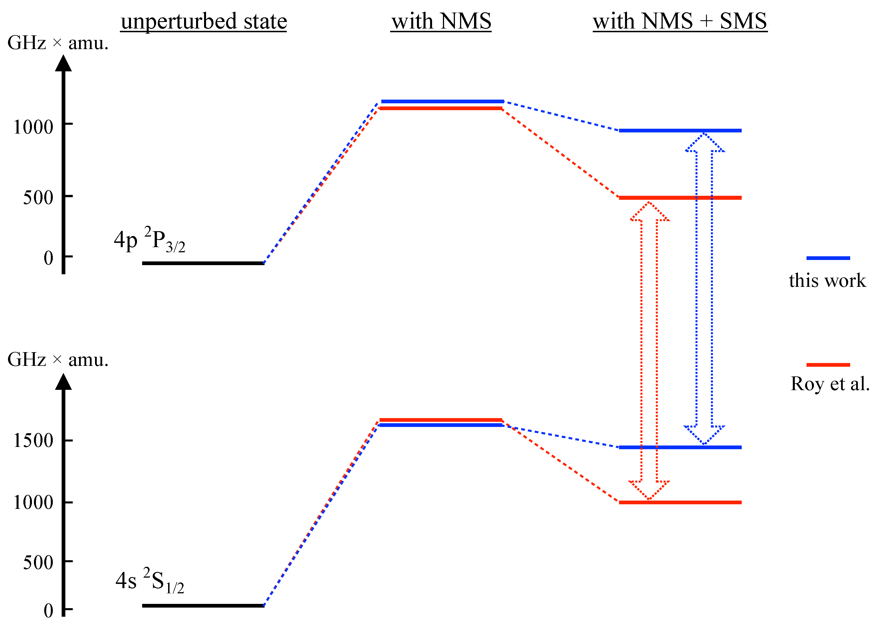
From the table we note that our results for the DHF calculations are close to the corresponding data in [14]. In the case of the RCC results, there is a good agreement with [14] for the normal mass shift pre-factor. However, the specific mass shift values diverge significantly. This is also illustrated in Figure 1.
The figure shows the perturbative contributions of NMS and SMS for the D2 line, as computed in [14] and in this work. The discrepancy in calculated SMS values is evident. For an analysis of the shift of the spectral line, this difference is partially obscured by the fact that the results diverge in the same directions for both the upper and lower level, and also by the dominant contribution from the NMS.
In a comparison between our RCCSD and RCCSD(T) results, a systematic difference is seen for the NMS and SMS components. This shows that triple excitations are important for optimum accuracy, but it is likely that their simplified inclusion, as applied here, overcompensates for their omission in RCCSD.
Spectral Lines
From the data in Table 2, we have derived isotope shifts for the involved spectral lines, for the specific pair of isotopes Ca and Ca. This includes the D1 (397 nm) and D2 (393 nm) lines, the coupling between the 4p and the metastable 3d levels (with ; at 866 nm, 854 nm, and 850 nm) and also the electric dipole forbidden 4s-3d transitions (733 nm and 729 nm). The latter are weakly coupled by an electric quadrupole (E2) moment. The perspective of the data from the view of spectral lines facilitates comparisons not only with [12,14], but also other theoretical works, such as Berengut et al. [13]. This is disseminated in Table 3, in which we also include comparisons with the experimental works Nörtershäuser et al. [7] and Garcia-Ruiz et al. [9].
The data are presented using the following convention: We calculate our shifts from Ca to Ca () by subtracting the individual shifts calculated for Ca from the ones for Ca, and with spectral line frequencies consistently being defined as: , , and . We subsequently apply the necessary sign adjustments to cited data to enable pertinent comparisons.
For the different computational methods we have applied, the comparison with the empiric data clearly indicates that our *DHF values give less accurate results than the RCC ones. This is expected, since a *DHF calculation must be truncated somewhere. For the RCC calculations, the ones including the limited form of the triple excitations agrees well with experimental values, for the four cases for which we have comparative data. Our two RCC results for the D2 line, as well as the works [12,13,14], are within 10–20% of the experimental value in [9] for the total isotope shift. For the three fine-structure lines of the 3d→4p transition, there is an excellent agreement between our RCC values and the measured ones in [7] (1–2%).
For the field shift, our RCC results agrees with [12] in absolute value, but has opposite signs. This does not appear to be due to different sign conventions. A possible explanation is an inconsistency in sign definitions in [12]. Indeed, the difference in the total isotope shift between [12] and our data (and incidentally also with experimental results) is not far from twice the values of calculated field shifts. There is a significant discrepancy between our field shift data and that in [14].
Among the other theoretical works, the NMS contribution can only be extracted from [14] and only for the D1 and D2 lines. The differences are of the order of 10%. Our SMS data agrees well with [13] for the s→d and p→d lines, which are strongly dominated by the large shift of the 3d levels (seen in Table 2). For s→p, the SMS impact on the spectral line is small. This is due to the effect of having the same sign and same order of magnitude for both upper and lower level, as shown in Figure 1.
For further direct comparisons with experimental values from [3,7,8,9,10], and with [12,14], we compile in Table 4 the total isotope shifts for a range of isotopes, using Ca as the reference. Our data is calculated from the pre-factors in Table 2.
Our data agrees very well (0.5–2%) with the empiric ones in [7] for . For this spectral line, the isotope shift is dominated by the SMS contribution. This is because the NMS shift is of the same order, and the same sign, for both P and D states (see Table 2). This makes the shift of the spectral line moderate. In contrast, the D states have SMS-shifts that are about an order of magnitude larger than those for the P states. For , the agreements is less good (ranging from 1% to 13%), and for almost all isotopes our RCCSD and RCCSD(T) data straddles the experimental numbers in [9]. This indicates again the importance of fully including triple excitations for obtaining optimum numerical results.
For the and , the agreement is good with [3] (from 0.1% to about 4%) and shows that this is a good starting point for more elaborate calculations, fully taking into account triple excitations.
4. Conclusions
We have investigated isotope shift constants for the field shift, normal mass shift, and specific mass shift of the first five low-lying states of the singly charged calcium ion by performing ab initio calculations in the finite-field procedure using the relativistic coupled-cluster theory. In contrast to earlier calculations, our results show that the final results for the individual states are indeed in reasonable agreement with the values obtained in the expectation value evaluation approach. The orbital relaxation effects to the isotope shift constants are found to be quite significant in the mean-field calculation. We also noticed that the finite-field approach produces large differences in the results between the fine-structure partner states, whereas such discrepancies are found to be quite small in the expectation value evaluation approach. This suggests the use of another potential method, for example normal coupled-cluster theory, which satisfies the biorthogonality condition and Hellmann–Feynman theorem, for minimising the numerical uncertainties of the finite-field approach for accurate determination of the isotope shift constants. Finally, we have applied our ab initio results to estimations of the isotope shifts of the , , and transitions of the calcium ion and compared them with the available high-precision measurements.
Author Contributions
A.K., A.D. and B.K.S. participated in discussions, analysing the results, and preparing the manuscript. All authors have read and agreed to the published version of the manuscript.
Funding
This research received no external funding.
Institutional Review Board Statement
Not applicable.
Informed Consent Statement
Not applicable.
Data Availability Statement
Acknowledgments
The computations were carried out using the Vikram-100 high-performance computing facility at the Physical Research Laboratory, Ahmedabad, India.
Conflicts of Interest
The authors declare no conflict of interest.
References
- Batiz-Hernandez, H.; Bernheim, R.A. Chapter 2 The isotope shift. Prog. Nucl. Magn. Reson. Spectrosc. 1967, 3, 63. [Google Scholar] [CrossRef]
- Heilig, K.; Steudel, A. Changes in mean-square nuclear charge radii from optical isotope shifts. At. Data Nucl. Data Tables 1974, 14, 613–638. [Google Scholar] [CrossRef]
- Solaro, C.; Meyer, S.; Fisher, K.; Berengut, J.C.; Fuchs, E.; Drewsen, M. Improved Isotope-Shift-Based Bounds on Bosons beyond the Standard Model through Measurements of the 2D3/2–2D5/2 Interval in Ca+. Phys. Rev. Lett. 2020, 125, 123003. [Google Scholar] [CrossRef] [PubMed]
- Henley, E.M.; Garcia, A. Subatomic Physics, 3rd ed.; World Scientific: Singapore, 2007. [Google Scholar]
- Pradhan, A.; Nahar, S. Atomic Astrophysics and Spectroscopy; Cambridge University Press: Cambridge, UK, 2011. [Google Scholar]
- Vermeeren, L.; Silverans, R.E.; Lievens, P.; Klein, A.; Neugart, R.; Schulz, C.; Buchinger, F. Ultrasensitive radioactive detection of collinear-laser optical pumping: Measurement of the nuclear charge radius of 50Ca. Phys. Rev. Lett. 1992, 68, 1679. [Google Scholar] [CrossRef] [PubMed]
- Nörtershäuser, W.; Blaum, K.; Icker, K.; Müller, P.; Schmitt, A.; Wendt, K.; Wiche, B. Isotope shifts and hyperfine structure in the 3d 2Dj →3d 2Pj transitions in calcium II. Eur. Phys. J. D 1998, 2, 33. [Google Scholar]
- Gorges, C.; Blaum, K.; Frömmgen, N.; Geppert, C.; Hammen, M.; Kaufmann, S.; Krämer, J.; Krieger, A.; Neugart, R.; Sánchez, R.; et al. Isotope shift of 40,42,44,48Ca in the 4s 2S1/2→ 4p 2P3/2 transition. J. Phys. At. Mol. Opt. Phys. 2015, 48, 245008. [Google Scholar] [CrossRef]
- Garcia Ruiz, R.F.; Bissel, M.L.; Blaum, K.; Ekström, A.; Frömmgen, N.; Hagen, G.; Hammen, M.; Hebeler, K.; Holt, J.D.; Jansen, G.R.; et al. Unexpectedly large radii of neutron-rich calcium isotopes. Nat. Phys. 2016, 12, 594. [Google Scholar] [CrossRef] [Green Version]
- Müller, P.; König, K.; Imgram, P.; Krämer, J.; Nörtershäuser, W. Collinear laser spectroscopy of Ca+: Solving the field-shift puzzle of the 4s2S1/2→4p2P1/2,3/2 transitions. Phys. Rev. Research 2020, 2, 043351. [Google Scholar] [CrossRef]
- Mårtensson-Pendrill, A.M.; Ynnerman, A.; Warston, H.; Vermeeren, L.; Silverans, R.E.; Klein, A.; Neugart, R.; Schulz, C.; Lievens, P.; The ISOLDE Collaboration. Isotope shifts and nuclear-charge radii in singly ionized 40–48Ca. Phys. Rev. A 1992, 45, 4675. [Google Scholar] [CrossRef] [PubMed] [Green Version]
- Safronova, M.S.; Johnson, W.R. Third-order isotope-shift constants for alkali-metal atoms and ions. Phys. Rev. A 2001, 64, 052501. [Google Scholar] [CrossRef] [Green Version]
- Berengut, J.C.; Dzuba, V.A.; Flambaum, V.V. Isotope-shift calculations for atoms with one valence electron. Phys. Rev. A 2003, 68, 022502. [Google Scholar] [CrossRef] [Green Version]
- Roy, S.; Majumder, S. Ab initio estimations of the isotope shift for the first three elements of the K isoelectronic sequence. Phys. Rev. A 2015, 92, 012508. [Google Scholar] [CrossRef]
- King, W.H. Isotope Shifts in Atomic Spectra; Springer: New York, NY, USA, 1984. [Google Scholar]
- Kastberg, A. Structure of Multielectron Atoms; Springer: Cham, Switzerland, 2020. [Google Scholar]
- Lindgren, I.; Morrison, J. Atomic Many-Body Theory, 2nd ed.; Springer: Berlin, Germany, 1986. [Google Scholar]
- Shavitt, I.; Bartlett, R. Many-Body Methods in Chemistry and Physics; Cambridge University Press: Cambridge, UK, 2009. [Google Scholar]
- Monkhorst, H.J. Calculation of properties with the coupled-cluster method. Int. J. Quantum Chem. 1977, 12, 421. [Google Scholar] [CrossRef]
- Bishop, R.F. The coupled cluster method. In Microscopic Quantum Many-Body Theories and Their Applications; Navarro, J., Polls, A., Eds.; Springer: Heidelberg, Germany, 1997; p. 1. [Google Scholar]
- Sahoo, B.; Vernon, A.; Garcia Ruiz, R.; Binnersley, C.; Billowes, J.; Bissell, M.; Cocolios, T.; Farooq-Smith, G.; Flanagan, K.; Gins, W.; et al. Analytic response relativistic coupled-cluster theory: The first application to indium isotope shifts. New J. Phys. 2020, 22, 012001. [Google Scholar] [CrossRef] [Green Version]
- Sahoo, B.K.; Das, B.P.; Mukherjee, D. Relativistic coupled-cluster studies of ionization potentials, lifetimes, and polarizabilities in singly ionized calcium. Phys. Rev. A 2009, 79, 052511. [Google Scholar] [CrossRef] [Green Version]
- Sahoo, B.K.; Das, B.P. Theoretical studies of the long lifetimes of the 6d2D3/2,5/2 states in Fr: Implications for parity-nonconservation measurements. Phys. Rev. A 2015, 92, 052511. [Google Scholar] [CrossRef]
- Sahoo, B.K. Conforming the measured lifetimes of the 5d2D3/2,5/2 states in Cs with theory. Phys. Rev. A 2016, 93, 022503. [Google Scholar] [CrossRef] [Green Version]
- Kramida, A.; Ralchenko, Y.; Reader, J.; NIST ASD Team. NIST Atomic Spectra Database (Ver. 5.3). 2018. Available online: http://physics.nist.gov/asd (accessed on 14 July 2019).
Figure 1.
Illustration of calculated mass shifts for the and levels obtained by the RCCSD method, in this work and in [14]. Although the calculated shifts in the two works are distinctly different, the resulting shift of an observed spectral line (which is the experimental observable) is similar for both calculations (498.6 GHz×amu for [14] and 420.69 GHz×amu for the present work).


Table 1.
Comparison of electron affinity values (in cm) from the calculations (as detailed in Section 2 and Equations (3) and (4)) with tabulated data. The latter values are quoted from the NIST database [25]. The three columns for the calculated values correspond to the different methods described in Section 2.
| Atomic State | DHF | RCCSD | RCCSD(T) | Empiric Data [25] |
|---|---|---|---|---|
| 91,440.02 | 95,883.58 | 95,444.94 | 95,751.87 | |
| 72,618.65 | 81,711.38 | 80,750.57 | 82,101.68 | |
| 72,594.55 | 81,631.34 | 80,670.66 | 82,040.99 | |
| 68,036.45 | 70,610.56 | 70,377.89 | 70,560.36 | |
| 67,836.79 | 70,378.86 | 70,149.40 | 70,337.47 |
Table 2.
Isotope shift pre-factors comparison for Ca II as obtained with different numerical calculation methods, compared to previous theoretical work in [12,14]. Abbreviations are explained in the text.
| This Work | Ref. [14] | Ref. [12] | ||||||
|---|---|---|---|---|---|---|---|---|
| Atomic State | DHF | DHF | RCCSD | RCCSD(T) | DHF | RCCSD | DHF | RMBPT |
| Field Shift (MHz × fm) | ||||||||
| 0 | 111.8 | |||||||
| 0 | 111.2 | |||||||
| 19.6 | ||||||||
| 0 | 19.9 | |||||||
| NMS (GHz × amu) | ||||||||
| 2383.86 | ||||||||
| 5494.38 | ||||||||
| 5479.22 | ||||||||
| 1619.66 | ||||||||
| 1611.92 | ||||||||
| SMS (GHz × amu) | ||||||||
Refers to the DHF values without accounting for the orbital relaxation effects.
Table 3.
Comparison of isotope shifts for various spectral lines between different numerical and experimental data for the isotope pair 40Ca II and 43Ca II, , in MHz. For this work, the three columns refer to data calculated using: a. *DHF, b. RCCSD, and c. RCC SD(T), as explaind in the text.
Table 3.
Comparison of isotope shifts for various spectral lines between different numerical and experimental data for the isotope pair 40Ca II and 43Ca II, , in MHz. For this work, the three columns refer to data calculated using: a. *DHF, b. RCCSD, and c. RCC SD(T), as explaind in the text.
| Spectral Line | This Work | Theory | Experiments | |||||
|---|---|---|---|---|---|---|---|---|
| a | b | c | [14] | [13] | [12] | [7] | [8] | |
| Field Shift (MHz) | ||||||||
| 47 | ||||||||
| 47 | ||||||||
| NMS (MHz) | ||||||||
| SMS (MHz) | ||||||||
| 22 | ||||||||
| 3479 | ||||||||
| 3507 | ||||||||
| 3492 | ||||||||
| Total (MHz) | ||||||||
| 591 | ||||||||
| 592 | ||||||||
| 3843 | ||||||||
| 3844 | ||||||||
| 3835 | ||||||||
Table 4.
Derived isotope shifts for a series of isotopes, using Ca as reference, for the dipole allowed transitions , , and as well as for the and transitions. The data are in MHz, and are compared to other theoretical works and experiments. The columns are labelled as in Table 3.
Table 4.
Derived isotope shifts for a series of isotopes, using Ca as reference, for the dipole allowed transitions , , and as well as for the and transitions. The data are in MHz, and are compared to other theoretical works and experiments. The columns are labelled as in Table 3.
| this work | theory | experiment | ||||||
| a | b | c | [14] | [12] | [10] | |||
| (15) | ||||||||
| 591 | ||||||||
| this work | theory | experiments | ||||||
| a | b | c | [14] | [12] | [9] | [8] | [10] | |
| 592 | ||||||||
| this work | theory | experiment | ||||||
| a | b | c | [12] | [7] | ||||
| 3843 | ||||||||
| this work | experiment | |||||||
| a | b | c | [3] | |||||
| 10,003.130 (2) | ||||||||
| this work | experiment | |||||||
| a | b | c | [3] | |||||
Publisher’s Note: MDPI stays neutral with regard to jurisdictional claims in published maps and institutional affiliations. |
© 2021 by the authors. Licensee MDPI, Basel, Switzerland. This article is an open access article distributed under the terms and conditions of the Creative Commons Attribution (CC BY) license (https://creativecommons.org/licenses/by/4.0/).
Share and Cite
MDPI and ACS Style
Dorne, A.; Sahoo, B.K.; Kastberg, A. Relativistic Coupled-Cluster Calculations of Isotope Shifts for the Low-Lying States of Ca II in the Finite-Field Approach. Atoms 2021, 9, 26. https://0-doi-org.brum.beds.ac.uk/10.3390/atoms9020026
AMA Style
Dorne A, Sahoo BK, Kastberg A. Relativistic Coupled-Cluster Calculations of Isotope Shifts for the Low-Lying States of Ca II in the Finite-Field Approach. Atoms. 2021; 9(2):26. https://0-doi-org.brum.beds.ac.uk/10.3390/atoms9020026
Chicago/Turabian StyleDorne, Anaïs, Bijaya K. Sahoo, and Anders Kastberg. 2021. "Relativistic Coupled-Cluster Calculations of Isotope Shifts for the Low-Lying States of Ca II in the Finite-Field Approach" Atoms 9, no. 2: 26. https://0-doi-org.brum.beds.ac.uk/10.3390/atoms9020026
Note that from the first issue of 2016, this journal uses article numbers instead of page numbers. See further details here.