Methods for Line Shapes in Plasmas in the Presence of External Electric Fields

Abstract

Line broadening is usually dominated by interactions of an atomic system with a stochastic, random medium. When, in addition to the random medium, a non-random field (such as a laser) is applied, the line profile may be modified in significant ways. The present work discusses these modifications and the methods to deal with them.

1. Introduction

Apart from natural broadening, line broadening of an atomic system requires a stochastic, random medium [1]. Pressure broadening in particular involves the interactions of the atomic system with the random medium. When, in addition to the random medium, a non-random electric or magnetic field field, either externally or internally generated, is applied, the line profile may be modified in significant ways. Specifically:

The first effect, usually neglected, is that the particle trajectories (or, in quantum terms the dielectric function) and distribution functions may be affected. We know that this can have an effect on the collision operators and lineshapes because we have already seen that these differ for say straight line and hyperbolic trajectories. This effect is often neglected (but see [2] for electric and for example [3,4] for magnetic fields) partly because it is hard to treat and partly because if the memory loss (inverse halfwidth) timescale is short compared to the electric field period or the cyclotron frequency is small compared to the line width for magnetic fields, one does not expect a significant effect due to trajectory modification.

The second effect is that, even if trajectories are not modified at all, the potential in the Schrödinger equation is modified because of the dressing of the interaction by the external (for example laser) field. For an external laser field, this may result in the dressed emitter-perturber interaction V(t) oscillating rapidly on the memory loss time scale. This means that because the dressed interaction changes sign rapidly, so does dU/dt and memory loss may be drastically inhibited [5,6]. The parameters of the external field determine exactly how the plasma-emitter interaction is dressed by the external field and if it then oscillates fast on the autocorrelation function C(t), i.e., the Fourier transform of the lineshape, time scale [7], decay of C(t) is inhibited and as a result the line narrows.

The third effect, first investigated by Blokhintsev [8], is that sattelites may appear, which is an effect that is medium-independent and only related to the external field (i.e., one encounters them even without a medium, except that these sattelites are then $\delta$-functions).

From a practical point of view this creates interesting opportunities for (X-ray laser in the case of plasmas) laser-based control, i.e., using a laser to reduce the line width and hence increase the gain, or arrange for merging sattelites so as to increase the line width and hence delay saturation. In the more general case the external laser may be used to dress the medium and affect whatever mechanism affects medium pressure broadening (excluding thermal, i.e., Doppler broadening). Additional diagnostic possibilities when a static field is present in a direction perpendicular to the oscillatory field have also been suggested [9,10,11] and will be briefly discussed here. However, a detailed analysis of specific experimental results is outside the scope of the present work and will be done separately.

2. Theoretical Formulation

The line profile in direction $\mathbf{e}$ is:

$$L_{\mathbf{e}}\left(\omega \right)=\left\{li{m}_{T\to \infty }\frac{1}{2\pi T}{\int }_{-T/2}^{T/2}d{t}_1{e}^{-i\omega t_1}{\mathbf{d}}_{\mathbf{e}{\alpha }_0\beta }\left(t_1\right){\int }_{-T/2}^{T/2}d{t}_2{e}^{i\omega t_2}{·\mathbf{d}}_{\mathbf{e}\beta {\alpha }_0}\left(t_2\right)\right\}$$

(1)

with $\{\dots \}$ the usual plasma average, d the dipole moment and ${\alpha }_0,\beta$ in principle complete sets of states. The density matrix has been assumed to be trivial. This may be written as (by using $t=t_2-t_1$):

$$\begin{array}{cc}& L_{\mathbf{e}}\left(\omega \right)=li{m}_{T\to \infty }\left\{{\int }_{-T/2}^{T/2}\frac{d{t}_1}{2\pi T}{\mathbf{d}}_{\mathbf{e}{\alpha }_0\beta }\left(t_1\right){\int }_{-T/2}^{T/2}dt{e}^{i\omega t}{·\mathbf{d}}_{\mathbf{e}\beta {\alpha }_0}(t+t_1)\right\}\\ \hfill & =li{m}_{T\to \infty }\frac{1}{2\pi T}\left\{{\int }_{-T/2}^{T/2}d{t}_1{\mathbf{d}}_{\mathbf{e}{\alpha }_0\beta }\left(t_1\right){\int }_{-\infty }^{\infty }dt{e}^{i\omega t}{·\mathbf{d}}_{\mathbf{e}\beta {\alpha }_0}(t+t_1)\right\}\end{array}$$

(2)

If we use the interaction picture with the 0th order Hamiltonian being the atomic plus external field Hamiltonian and U and $U_0$ the interaction and unperturbed time evolution operators (U-matrices) respectively:

$$\mathbf{d}\left(t\right)=U^{†}\left(t\right)U^{0†}\left(t\right)\mathbf{d}{U}^0\left(t\right)U\left(t\right)$$

(3)

we have, since we have a Trace($\langle {\alpha }_0|\dots |{\alpha }_0\rangle$):

$$\begin{array}{cc}& L_{\mathbf{e}}\left(\omega \right)=li{m}_{T\to \infty }\frac{1}{2\pi T}{\int }_{-T/2}^{T/2}d{t}_1{\int }_{-\infty }^{\infty }dt{e}^{i\omega t}\\ \hfill & \langle {\alpha }_0\left|\right\{U^{†}\left(t_1\right)U^{0†}\left(t_1\right){\mathbf{d}}_{\mathbf{e}}{U}^0\left(t_1\right)U\left(t_1\right)U^{†}(t+t_1)\\ \hfill & U^{0†}(t+t_1){\mathbf{d}}_{\mathbf{e}}{U}^0(t+t_1)U(t+t_1)\left\}\right|{\alpha }_0\rangle \end{array}$$

(4)

Using the cyclic property of the trace and the fact that $U^{†}=U^{-1}$, recalling that $U\left(t\right)=U(t,0)$ (from time 0 to time t) we have

$$U\left(t_1\right)U^{†}(t+t_1)=U(t_1,0){\left[U(t_1+t,t_1)U(t_1,0)\right]}^{-1}=U^{†}(t_1+t,t_1)$$

(5)

$$U(t+t_1)U^{†}\left(t_1\right)=U(t+t_1,t_1)U(t_1,0)U^{-1}(t_1,0)=U(t+t_1,t_1)$$

(6)

Therefore the line profile along the e direction is:

$$\begin{array}{cc}& L_{\mathbf{e}}\left(\omega \right)=li{m}_{T\to \infty }\frac{1}{2\pi T}{\int }_{-T/2}^{T/2}d{t}_1{\int }_{-\infty }^{\infty }dt{e}^{i\omega t}\langle {\alpha }_0\left|\right\{U^{0†}\left(t_1\right){\mathbf{d}}_{\mathbf{e}}\\ \hfill & U^0\left(t_1\right)U^{†}(t_1+t,t_1)U^{0†}(t+t_1){\mathbf{d}}_{\mathbf{e}}{U}^0(t+t_1)U(t+t_1,t_1)\left\}\right|{\alpha }_0\rangle \end{array}$$

(7)

Then using complete sets of states (in practice $\alpha ,{\alpha }^{\prime }\dots$ refer to upper and $\beta ,{\beta }^{\prime },\dots$ to lower level states):

$$\begin{array}{cc}& L_{\mathbf{e}}\left(\omega \right)=li{m}_{T\to \infty }\frac{1}{2\pi T}{\int }_{-T/2}^{T/2}d{t}_1{\int }_{-\infty }^{\infty }dt{e}^{i\omega t}\\ \hfill & \{U_{{\alpha }_0\alpha }^{0†}\left(t_1\right){\mathbf{d}}_{\mathbf{e}\alpha \beta }·U_{\beta {\beta }_0}^0\left(t_1\right)U_{{\beta }_0{\beta }_1}^{†}(t_1+t,t_1)U_{{\beta }_1{\beta }^{\prime }}^{0†}(t+t_1)\\ \hfill & {\mathbf{d}}_{\mathbf{e}{\beta }^{\prime }{\alpha }^{\prime }}{U}_{{\alpha }^{\prime }{\alpha }_1}^0(t+t_1)U_{{\alpha }_1{\alpha }_0}(t+t_1,t_1)]\\ \hfill & =li{m}_{T\to \infty }\frac{1}{2\pi T}{\int }_{-T/2}^{T/2}d{t}_1{\int }_{-\infty }^{\infty }dt{e}^{i\omega t}\\ \hfill & \left\{U_{{\alpha }_1{\alpha }_0}(t+t_1,t_1)U_{{\beta }_0{\beta }_1}^{†}(t_1+t,t_1)\right\}{U}_{{\alpha }_0\alpha }^{0†}\left(t_1\right){\mathbf{d}}_{\mathbf{e}\alpha \beta }·\\ \hfill & U_{\beta {\beta }_0}^0\left(t_1\right)U_{{\beta }_1{\beta }^{\prime }}^{0†}(t+t_1){\mathbf{d}}_{\mathbf{e}{\beta }^{\prime }{\alpha }^{\prime }}{U}_{{\alpha }^{\prime }{\alpha }_1}^L(t+t_1)\end{array}$$

(8)

Note that the only part involving the medium is $\left\{U_{{\alpha }_1{\alpha }_0}(t+t_1,t_1)U_{{\beta }_0{\beta }_1}^{†}(t_1+t,t_1)\right\}$, as everything else involves only the time evolution of the atomic system $U^0$ in the presence of only the laser, but not the medium. If the C(t) time scale (i.e., the times involved) is large compared to the deterministic field period this should be independent of the time origin and hence may be replaced by $\left\{U_{{\alpha }_1{\alpha }_0}\left(t\right)U_{{\beta }_0{\beta }_1}^{†}\left(t\right)\right\}$. Numerically, the interaction picture is perhaps more transparent and attractive because of the identification of peaks and intensities via the plasma-independent part (a and b below) and because solving the Schrödinger equation for the dressed interaction is advantageous, as the changes in the U-matrix hapening on a given time scale are typically much smaller and hence the integration faster. In other words, the alternative approach is to solve for each random perturber configuration, the Schrödinger equation in the combined random plus nonrandom fields, which evolution may be dominated by the nonrandom fields and to extract the peaks from the Fourier transform and this has been done in previous Spectral Line Shapes Workshops [12].

We can therefore write the line profile as a product of (a) dipole matrix D, (b) a plasma independent matrix S and (c) a plasma dependent quantity:

$$L_{\mathbf{e}}\left(\omega \right)=D_{\alpha \beta {\beta }^{\prime }{\alpha }^{\prime }}{\int }_{-\infty }^{\infty }dt{e}^{i\omega t}{S}_{{\alpha }_0{\alpha }_1{\beta }_1{\beta }_0\beta {\beta }^{\prime }{\alpha }^{\prime }\alpha }\left(t\right)\left\{U_{{\alpha }_1{\alpha }_0}\left(t\right)U_{{\beta }_0{\beta }_1}^{†}\left(t\right)\right\}$$

(9)

where the dipole term D is purely atomic,

$$D_{\alpha \beta {\beta }^{\prime }{\alpha }^{\prime }}={\mathbf{d}}_{\mathbf{e}\alpha \beta }{·\mathbf{d}}_{\mathbf{e}{\beta }^{\prime }{\alpha }^{\prime }}$$

(10)

and the plasma-independent (but laser-dependent) matrix S is:

$$\begin{array}{cc}& S_{{\alpha }_0{\alpha }_1{\beta }_1{\beta }_0\beta {\beta }^{\prime }{\alpha }^{\prime }\alpha }\left(t\right)=li{m}_{T\to \infty }\frac{1}{2\pi T}\\ \hfill & {\int }_{-T/2}^{T/2}d{t}_1{U}_{{\alpha }_0\alpha }^{0†}\left(t_1\right)U_{\beta {\beta }_0}^0\left(t_1\right)U_{{\beta }_1{\beta }^{\prime }}^{0†}(t+t_1)U_{{\alpha }^{\prime }{\alpha }_1}^0(t+t_1)\end{array}$$

(11)

S determines the sattelite structure and intensity, D determines the total line intensity and $\{\dots \}$ determines the broadening of each sattelite. In the case without a laser field, $U_{ij}^0\left(t\right)={\delta }_{ij}exp(-i{\omega }_{i}t)$ and S reduces to

$$S_{{\alpha }_0{\alpha }_1{\beta }_1{\beta }_0\beta {\beta }^{\prime }{\alpha }^{\prime }\alpha }\left(t\right)=e^{-ıt({\omega }_{{\alpha }^{\prime }}-{\omega }_{{\beta }^{\prime }})}\delta ({\omega }_{{\alpha }_0}-{\omega }_{{\beta }_0}-{\omega }_{{\alpha }^{\prime }}+{\omega }_{{\beta }^{\prime }}){\delta }_{{\alpha }_0{\alpha }^{\prime }}{\delta }_{\beta {\beta }_0}{\delta }_{{\alpha }^{\prime }{\alpha }_1}{\delta }_{{\beta }^{\prime }{\beta }_1}$$

(12)

Indeed, $U_0$ can be Fourier-analyzed, resulting in $\delta -functions$ if $U_0$ is periodic or shifted periodic (i.e., involing extra imaginary exponentials), resulting in a sattelite structure with repeated peaks. If not, then S is a broader structure. Note that no assumption has been made thus far (e.g., hydrogenic emitter of basis or functional form of the external field (for instance exactly harmonic), apart from $\left\{U_{ij}(t+t_1,t_1)U_{kl}^{†}(t+t_1,t_1)\right\}=\left\{U_{ij}\left(t\right)U_{kl}^{†}\left(t\right)\right\}$). To identify C(t) and also to reduce this expression to as basis-independent a form as possible, one may extract the “no laser” term $exp[-ıt({\omega }_{{\alpha }^{\prime }}-{\omega }_{{\beta }^{\prime }})]$ from S and write it separately. To do this, simply use again the interaction picture on the time evolution operator $U^0$, this time with the atomic Hamiltonian as unperturbed and the laser as the perturbation, i.e.,

$$U^0\left(t\right)=U^A\left(t\right)U^L\left(t\right)$$

(13)

with the A and L superscripts denoting atomic and Laser Hamiltonians, respectively.

With the states denoting atomic states and using the diagonality of $U^A$, S becomes:

$$S_{{\alpha }_0{\alpha }_1{\beta }_1{\beta }_0\beta {\beta }^{\prime }{\alpha }^{\prime }\alpha }\left(t\right)=e^{-ı({\omega }_{{\alpha }^{\prime }}-{\omega }_{{\beta }^{\prime }})t}{G}_{{\alpha }_0{\alpha }_1{\beta }_1{\beta }_0\beta {\beta }^{\prime }{\alpha }^{\prime }\alpha }\left(t\right)$$

(14)

with

$$\begin{array}{cc}& G_{{\alpha }_0{\alpha }_1{\beta }_1{\beta }_0\beta {\beta }^{\prime }{\alpha }^{\prime }\alpha }\left(t\right)=li{m}_{T\to \infty }\frac{1}{2\pi T}{\int }_0^{T}d{t}_1{U}_{{\alpha }_0{\alpha }_1}^{L†}\left(t_1\right)\\ \hfill & U_{{\beta }_1{\beta }_0}^L\left(t_1\right)U_{\beta {\beta }^{\prime }}^{L†}(t+t_1)U_{{\alpha }^{\prime }\alpha }^L(t+t_1)exp\left[ıt_1({\omega }_{{\alpha }_1}-{\omega }_{{\beta }_1}-{\omega }_{{\alpha }^{\prime }}+{\omega }_{{\beta }^{\prime }})\right]\end{array}$$

(15)

with $U^L$ determined by the Schroedinger equation:

$$\frac{d{U}^L}{dt}=-\frac{ı}{\hslash }{e}^{ıH_{A}t/\hslash }{V}_L\left(t\right)e^{-ıH_{A}t/\hslash }{U}^L\left(t\right)$$

(16)

with $V^L$ the laser-emitter interaction and $H_A$ the atomic Hamiltonian.

Therefore the final result for the line profile along the direction e is:

$$L_{\mathbf{e}}\left(\omega \right)=\sum _k{\int }_{-\infty }^{\infty }dt{e}^{i(\omega -{\omega }_{{\alpha }^{\prime }{\beta }^{\prime }})t}{C}_k\left(t\right)$$

(17)

with

$$C_k\left(t\right)=D_{\alpha \beta {\beta }^{\prime }{\alpha }^{\prime }}{G}_{{\alpha }_0{\alpha }_1{\beta }_1{\beta }_0\beta {\beta }^{\prime }{\alpha }^{\prime }\alpha }\left(t\right)\left\{U_{{\alpha }_1{\alpha }_0}\left(t\right)U_{{\beta }_0{\beta }_1}^{†}\left(t\right)\right\}$$

(18)

where k refers to each ${\alpha }^{\prime }\to {\beta }^{\prime }$ transition of interest. For example if we look at a hydrogenic line, the various ${\omega }_{{\alpha }^{\prime }{\beta }^{\prime }}$ could correspond to the different fine structure components.

3. Time-Periodic Fieds: Floquet Theory

Up until now the discussion has made no assumptions on the specific time-dependence of the external field. We now consider the case of time-periodic fields. In that case Floquet’s theorem shows that the U-matrix is a product of a time periodic matrix and an exponential matrix. From Equation (16) note that $U_L$ has a Floquet structure if $H_A$ is degenerate. In the more general case, $U_L$ itself does not have a Floquet structure, but the $U_0$-matrix for evolution in the presence of the time-independent atomic Hamiltonian plus periodic field does.

The spectrum (Equation (12) is determined by the eigenvalues (often called quasi-energies) of $F_0$ as well as its eigenvectors (often called modes). Floquet theory has been applied before for this problem [13,14]. The difference from the present approach is that in the works cited Floquet theory was applied in the context of the impact/unified(Liouville) theory, which in principle needs some approximation (typically perturbation theory) to compute the self-energy matrix. Floquet’s theorem (see Appendix A) shows that $U_0$ is the product of a periodic function $P\left(t\right)$ and an exponential:

$$U_0\left(t\right)=P\left(t\right)e^{ıBt}$$

(19)

with B constant and P periodic:

$$P\left(t\right)=\sum _{k=-\infty }^{\infty }{p}_k{e}^{ık\Omega t}$$

(20)

Hence we write: $e^{ıBt}=E{e}^{ı\Lambda t}{E}^{-1}$, with E the (time-independent) eigenvectors of B and $\Lambda$ a diagonal matrix with real eigenvalues. Unitarity means that $E^{-1}=E^{†}$ need not be computed. Reality of eigenvalues is simple to see on mathematical (e.g., since $e^{ıBT}=U\left(T\right)$ is unitary, then $BT$ must be Hermitian, i.e., B must be Hermitian) or, equivalently, physical grounds (if the eigenvalues had a negative imaginary part, $U(\infty )$ would diverge, while if it had a positive imaginary part, it would become 0, and thus result in population loss). If B is degenerate, as in hydrogen-like species with no fine structure and no external fields or consideration of quenching, then the case is trivial and B can effectively be absorbed in the choice of the line center frequency. We can rewrite Equation (19) as

$$U_0\left(t\right)=Z\left(t\right)e^{ı\Lambda t}{E}^{-1}$$

(21)

with the periodic matrix

$$Z\left(t\right)=P\left(t\right)E=\sum _{n=-\infty }^{\infty }{e}^{ı\Omega nt}{z}_n$$

(22)

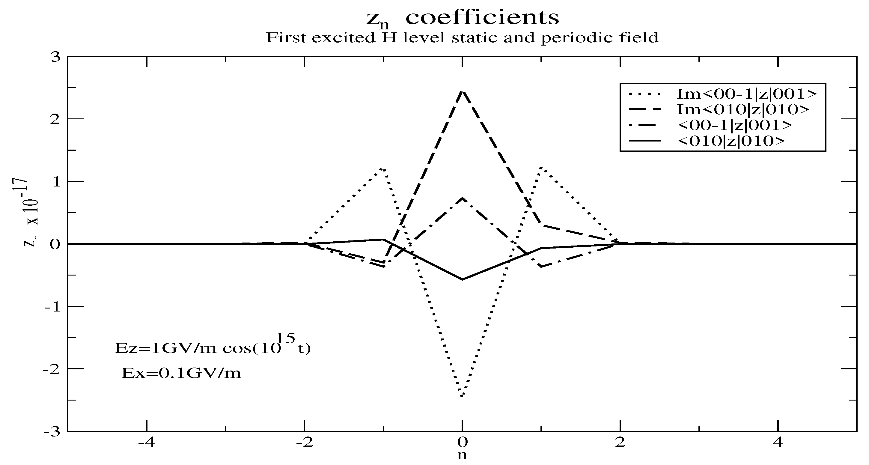
and the subscript n denoting the nth Fourier component of Z in the Fourier series expansion of the periodic function $Z\left(t\right)$. Figure 1 displays matrix elements of the constant matrices $z_n$ as a function of n.

The matrix S therefore gives rise to a sattelite structure, specifically, the satellite structure from Equation (12) reads:

$$\begin{array}{cc}& S_{{\alpha }_0{\alpha }_1{\beta }_1{\beta }_0\beta {\beta }^{\prime }{\alpha }^{\prime }\alpha }\left(t\right)=e^{ı\Omega t(p-l)}li{m}_{T\to \infty }\frac{1}{2\pi T}{\int }_{-T/2}^{T/2}d{t}_1\\ \hfill & E_{{\alpha }_0{\alpha }_2}^{-1†}{e}^{-ı{\lambda }_{{\alpha }_2}{t}_1}{z}_{{}_n{\alpha }_2\alpha }^{†}{z}_{m\beta {\beta }_2}{e}^{ı{\lambda }_{{\beta }_2}{t}_1}{E}_{{\beta }_2{\beta }_1}^{-1}{E}_{{\beta }_1{\beta }_3}^{-1†}{e}^{-ı{\lambda }_{{\beta }_3}(t+t_1)}{z}_{l{\beta }_3{\beta }^{\prime }}^{†}{z}_{p{\alpha }^{\prime }{\alpha }_3}{e}^{ı{\lambda }_{{\alpha }_3}(t+t_1)}{E}_{{\alpha }_3{\alpha }_1}^{-1}{e}^{ı\Omega (-n+m-l+p)}\\ \hfill & =e^{ıt[\Omega (p-l)+{\lambda }_{{\alpha }_3}-{\lambda }_{{\beta }_3}]}{E}_{{\alpha }_0{\alpha }_2}{z}_{{}_n{\alpha }_2\alpha }^{†}{z}_{m\beta {\beta }_2}{E}_{{\beta }_2{\beta }_1}^{-1}{E}_{{\beta }_1{\beta }_3}{z}_{l{\beta }_3{\beta }^{\prime }}^{†}{z}_{p{\alpha }^{\prime }{\alpha }_3}{E}_{{\alpha }_3{\alpha }_1}^{-1}\delta [\Omega (-n+m-l+p)+{\lambda }_{{\alpha }_3}-{\lambda }_{{\alpha }_2}+{\lambda }_{{\beta }_2}-{\lambda }_{{\beta }_3}]\end{array}$$

(23)

At this point it may be instructive to consider the plasma-independent term for directione

$$\begin{array}{cc}\hfill {\overline{S}}_{{\alpha }_0{\alpha }_1{\beta }_1{\beta }_0}=D_{\alpha \beta {\beta }^{\prime }{\alpha }^{\prime }}^{\mathbf{e}}{S}_{{\alpha }_0{\alpha }_1{\beta }_1{\beta }_0\beta {\beta }^{\prime }{\alpha }^{\prime }\alpha }\left(t\right)& ={\sum }_{nmlp}\delta [\Omega (-n+m-l+p)+{\lambda }_{{\alpha }_3}-{\lambda }_{{\alpha }_2}+{\lambda }_{{\beta }_2}-{\lambda }_{{\beta }_3}]\\ \hfill & E_{{\alpha }_0{\alpha }_2}{{\mathbf{R}}^{\mathbf{e}}}_{{\alpha }_2{\beta }_2}(n,m)E_{{\beta }_2{\beta }_0}^{†}{E}_{{\beta }_1{\beta }_3}{·{\mathbf{R}}^{\mathbf{e}}}_{{\alpha }_3{\beta }_3}^{†}(p,l)E_{{\alpha }_3{\alpha }_1}^{†}{e}^{ıt[(p-l)\Omega +{\lambda }_{{\alpha }_3}-{\lambda }_{{\beta }_3}]}\end{array}$$

(24)

with

$${{\mathbf{R}}^{\mathbf{e}}}_{\alpha \beta }(n,m)=z_{n\alpha {\alpha }^{\prime }}^{†}{\mathbf{d}}_{\mathbf{e}{\alpha }^{\prime }{\beta }^{\prime }}{z}_{m{\beta }^{\prime }\beta }$$

(25)

Note the mixture of Floquet exponents and (n, m, l, p) due to the imaginary exponential and the $\delta$ function.

This may be written as

$${\overline{S}}_{{\alpha }_0{\alpha }_1{\beta }_1{\beta }_0}=\sum _k\sum _{n=-\infty }^{\infty }{Q}_{nk}{e}^{ı(\Omega n+{\Delta }_k)t}$$

(26)

The point is that n runs over all integers, while k runs over the distinct combination k of differences in the upper-lower Floquet exponents. This results in a modified sattelite structure: If the plasma-dependent quantity $\left\{U_{{\alpha }_1{\alpha }_0}\left(t\right)U_{{\beta }_0{\beta }_1}^{†}\left(t\right)\right\}$ is Fourier-analyzed in terms of functions $u_j\left(\omega \right)$, then the profile qualitatively consists of linear combinations of $u_j(\omega -n\Omega -{\Delta }_k)$. In other words the total profile is the sum of a number of profiles, each with their own intensity (given by $Q_{nk}$), centers (given by $\Omega n+{\Delta }_k$) and widths and shifts (determined by decay of $\left\{U_{{\alpha }_1{\alpha }_0}\left(t\right)U_{{\beta }_0{\beta }_1}^{†}\left(t\right)\right\}$), as illustrated in Figure 2 and Figure 3, i.e.,

$$L^{\mathbf{e}}\left(\omega \right)=\sum _{nk}\int dt{C}_{nk}^{\mathbf{e}}\left(t\right)e^{ı(\omega -{\omega }_{nk})t}$$

(27)

with

$${\omega }_{nk}={\Omega }_n+{\Delta }_k$$

(28)

and remaining factors forming the autocorrelation function of this component in direction e.

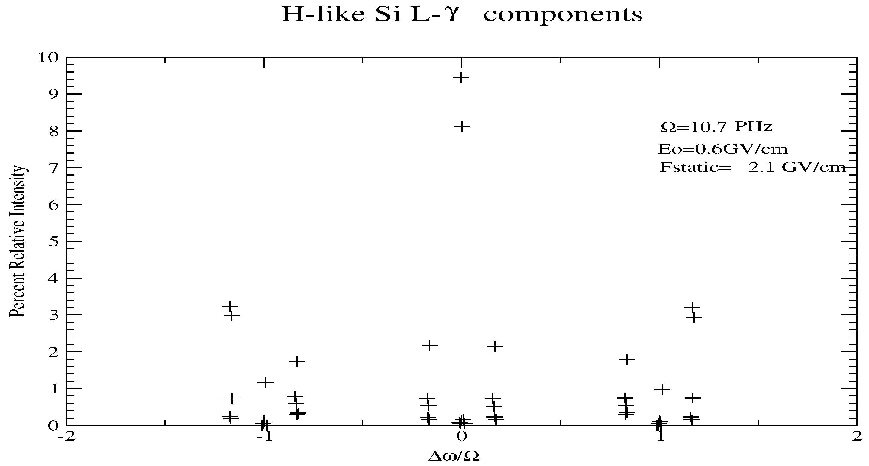
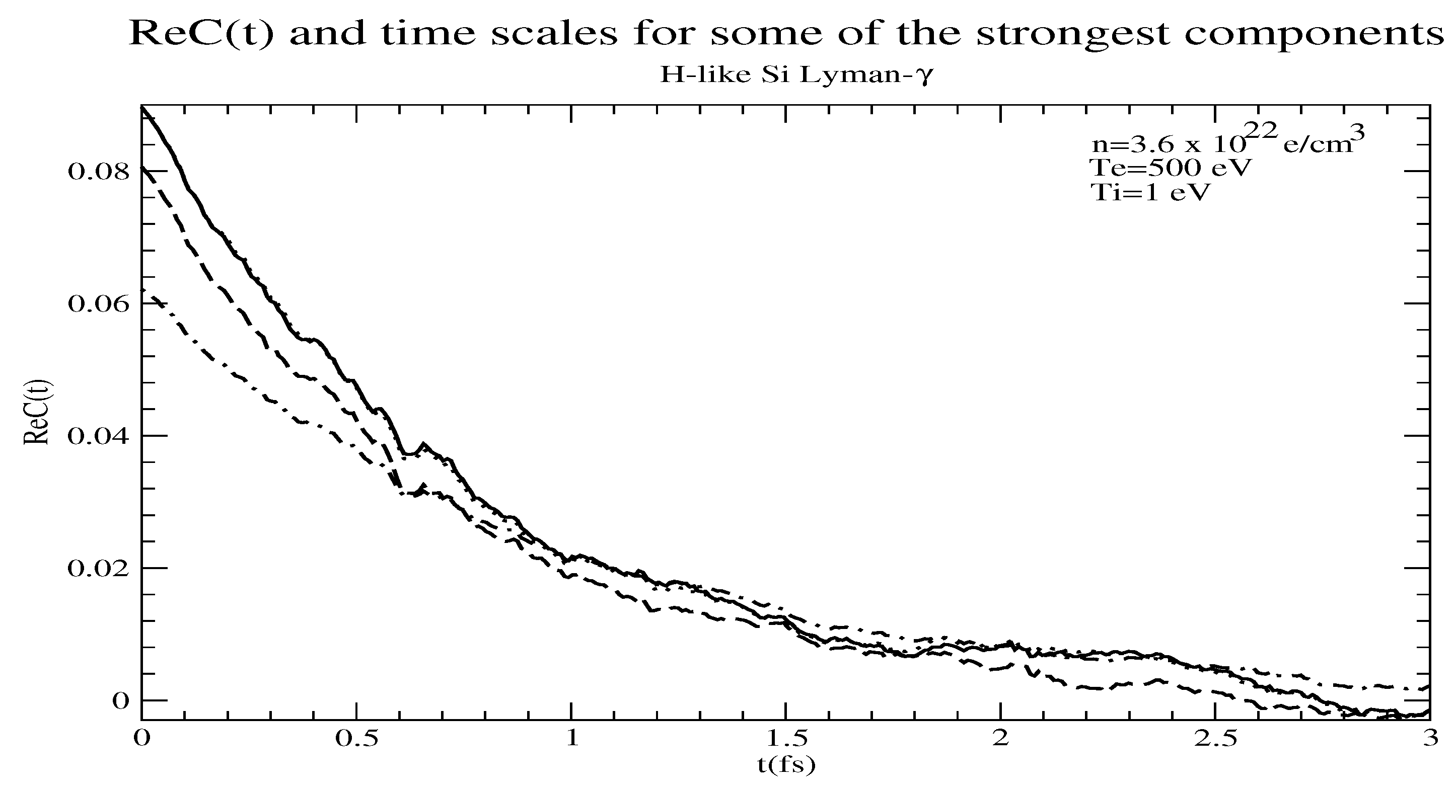
Figure 2 displays the positions and relative intensities of the various components $\Omega n+{\Delta }_k$ for H-like Si $L-\gamma$ under conditions similar to those described in Refs. [10,11]. The difference between the intensities can exceed many orders of magnitude. Figure 3 displays the real parts of $C_{nk}$ for some of the strongest components $nk$ for H-like Si $L-\gamma$ under conditions similar to those described in Refs. [10,11], namely electron density 3.6 × 10${}^{22}$ e/cc, electron and ion temperatures 500 and 1 eV respectively and a linearly polarized oscillatory field $E_{0}cos(\Omega t)$ with $E_0=0.6$ GV/cm and $\Omega =1.07\times {10}^{16}$ s${}^{-1}$, as well as a static field $F_{static}$ of magnitude 2.1 GV/cm in the direction perpendicular to the oscillatory field. Fine structure is included in the calculations. The sum of the autocorrelation functions in the parallel and perpendicular directions is displayed. The calculation used 100 plasma particle configurations and an impact tail [15] for long times was recognizable. Broadening by both electrons and ions was accounted for in the calculation shown.

If the outside field is not exactly periodic, it may still be Fourier-transformed. In that case we do not get exactly sattelites, but a more spread out structure on which the medium broadening will be superimposed.

3.1. Qualitative Remarks on the B-Matrix

The Floquet exponents $\lambda$ are typically produced by a time-independent breakdown of degeneracy, such as a constant Stark field or fine structure However, the $\lambda$ are not necessarily exactly equal to say the Stark shifts. The B-matrix is typically related to a time-independent term, as stated above. It is shown in Appendix B that B is identically 0 if we solve for a pure periodic field (monochromatic or not) with no time-independent term. Therefore, for degenerate cases, i.e., H-like species with no fine structure and in the no-quenching approximation, $B=e^{-ı\omega t}$ with $\hslash \omega$ the energy of the level in question; alternatively B may be taken as 0 if we measure energy differences from the line transition. If nontrivial (i.e., nondegenerate), B is related to a time-independent term in the Hamiltonian, and it makes no mathematical difference if this comes from the atomic Hamiltonian itself, or from a possible static field. To our knowledge the joint action of a static and an oscillatory field was first considered in [16,17].

Note that the B-matrix is never used directly; its eigenvalues and eigenvectors are all we need.

3.2. General Lineshape and Static Solutions

From the previous discussion, it is obvious that the profile will in general be a superposition of profiles centered at positions corresponding to combinations of n and k and intensities as specified by $Q_{nk}$. Depending on the width of these profiles (which $does$ in turn depend on the periodic field parameters) with respect to their separation, and the $Q_{nk}$ intensities, these may appear as either isolated or overlapping features. It should then be no surprise to see peaks and troughs in such profiles.

Although we will be dealing in detail with such predictions in a separate publication, note that if one assumes small plasma effects, i.e., $\left\{U_{{\alpha }_1{\alpha }_0}\left(t\right)U_{{\beta }_0{\beta }_1}^{†}\left(t\right)\right\}\approx {\delta }_{alph{a}_1{\alpha }_0}{\delta }_{{\beta }_0{\beta }_1}$ and a random but static electric field (internally generated, e.g., ion acoustic turbulence or static ion fields) in addition to the oscillatory field, the system (oscillatory plus static field) is still periodic and the previous results apply, except that the final profile involves an integral over the random static fields $\mathbf{F}$ and their distribution $W\left(\mathbf{F}\right)$:

$$\begin{array}{cc}\hfill L_{\mathbf{e}}\left(\omega \right)& ={\sum }_{kn}\int \mathbf{dF}W\left(\mathbf{F}\right){\int }_{-\infty }^{\infty }dt{e}^{i[\omega +\Omega n+{\Delta }_k\left(\mathbf{F}\right)]t}{Q}_{nk}^e\left(\mathbf{F}\right)\\ & ={\sum }_{kn}\int \mathbf{dF}W\left(\mathbf{F}\right)Q_{nk}^e\left(\mathbf{F}\right)\delta (\omega +n\Omega +{\Delta }_k\left(\mathbf{F}\right))\end{array}$$

(29)

where now $Q_{nk}$ is a scalar, after matrix multiplication with $\left\{U_{{\alpha }_1{\alpha }_0}\left(t\right)U_{{\beta }_0{\beta }_1}^{†}\left(t\right)\right\}$. Making use of

$$\delta \left(f\left(x\right)\right)=\sum _i\frac{\delta (x-x_i)}{|f^{\prime }\left(x_i\right)|}$$

(30)

with $x_i$ the roots of $f\left(x\right)=0$ (and its 3-dimensional generalization), this reads:

$$L_{\mathbf{e}}\left(\omega \right)=\sum _{nki}\frac{W\left({\mathbf{F}}_{\mathbf{i}}\right)Q_{nk}\left({\mathbf{F}}_{\mathbf{i}}\right)}{|\nabla {\Delta }_{nk}\left({\mathbf{F}}_{\mathbf{i}}\right)|}.$$

(31)

Note that ${\mathbf{F}}_{\mathbf{i}}$ are functions of $\omega$, as they are roots of $\omega +n\Omega +{\Delta }_k\left(\mathbf{F}\right)=0$. Some ${\Delta }_k$ may be unaffected by the static field (e.g., central components). For these of course, $\delta$-function profiles cannot be avoided in a static picture.

Additionally, note that irrespective of the exact form of W, $W\left(0\right)=0$. Then:

a

If ${\Delta }_{nk}$ is independent of ${\mathbf{F}}_{\mathbf{i}}$, we get the usual static results of $\delta$-functions for central components at the Blokhitsev positions or integer multiples of $\Omega$.

b

For $\omega =n\Omega$, the $\delta$-function argument is zero for ${\Delta }_{nk}\left({\mathbf{F}}_{\mathbf{i}}\right)=0$, which is typically satisfied for $F_i\approx 0$, at least for H-like species. However, then the distribution function $W\left(0\right)=0$ ensures a zero result which could show up as a dip. Hence in this view one might expect intensity drops and these should practically coincide with the Blokhintsev peaks at $n\Omega$ to the extent that $|{\Delta }_k|\ll \Omega$.

It should be stressed that static fields in plasmas are often wishful thinking: Of course one effect of a laser field is to dress the emitter-plasma interaction by an oscillatory function, which may oscillate rapidly and hence change the sign of the interaction in the Schrödinger equation and hence tend to keep $\left\{U_{{\alpha }_1{\alpha }_0}\left(t\right)U_{{\beta }_0{\beta }_1}^{†}\left(t\right)\right\}$ is “small”. However, some broadening mechanism will need to provide the memory loss and the dressing just descirbed will only delay the ultimate decay of C(t) and hence effectively increases the memory loss time (the inverse of the width) in the autocorrelation function. If some random static field is the dominant mechanism, this clearly cannot work for lines with a central component and for other lines it has to be strong enough to provide memory loss on a time scale where it is static. For a field to be considered constant (static) in this context, it must change on a time scale significantly longer than the autocorrelation function’s time scale. A field is static not because it is “large” or “small”, but because it varies little on the inverse HWHM time scale. This requires some broadening mechanism to provide this memory loss. The mechanism just discussed assumes that $\left\{U_{{\alpha }_1{\alpha }_0}\left(t\right)U_{{\beta }_0{\beta }_1}^{†}\left(t\right)\right\}\approx I$ on a time scale that the static field both does not change and has produced an appreciable memory loss. We have just explained that the profile is a sum of profiles, each with its own central position, intensity and width and shift and is never strictly zero.

3.3. Numerical Floquet Solution

For a periodic field (such as a laser), use of Floquet theory represents a way to significantly optimize the calculation: Compared to solving the Schrödinger equation in the external plus plasma particle field, which may be dominated by the external field for high field amplitudes, the alternative algorithm can be significantly more efficient:

The point is that if B (actually its eigenvalues and eigenvectors) is reliably computed and $P\left(t\right)$ is determined in [0,T], we effectively have computed the plasma-unperturbed evolution operator for all times. Since the periodic field intensity may well exceed the plasma microfield, even by orders of magnitude, if we solve for the total (deterministic laser plus stochastic plasma) field, the change over a given time step can de dominated by the deterministic field. Thus, it is numerically quite convient to use the interaction picture after having solved the 0th order Hamiltonian with the periodic field; it also directly identifies the sattelite positions. In addition, if a numerical solution is necessary, it is important that we only need $U_0$ for the laser period, not the time of interest for C(t), which may be much larger.

3.3.1. Direct B Eigendecomposition

Direct B eigendecomposition is conceptually simple and involves the following steps:

• Determination of B. Since $U_0\left(0\right)=I=P\left(0\right)=P\left(T\right),U_0\left(T\right)=e^{-ıBT}$, compute once and for all $U_0\left(T\right)$, i.e., the time evolution for one period in the presence of the periodic field and no plasma. Since U(T) must be unitary, accuracy is typically important and since the problem is typically stiff, a geometric integrator, preserving unitarity, should be used [18].
• Diagonalize $U_0\left(T\right)=E{e}^{ı\Lambda T}{E}^{-1}$ to obtain the eigenvalue decomposition of B once and for all. Since $U_0\left(T\right)$ is unitary, the best way is to compute the Schur factorization: $U\left(T\right)=XT{X}^{†}$, where X is unitary, and since $U\left(T\right)$ is unitary, the upper triangular matrix T is unitary and hence diagonal.Thus the columns of X are eigenvectors of $U\left(T\right)$ and form an orthonormal basis.
• Compute, also once and for all, the satellite structure: For all distinct eigenvalues ${\lambda }_i$ of B, consider all sattelite positions ${\Delta }_i+n\Omega$, for all integer n resulting in satellite position in the region of interest, where ${\Delta }_i$ refers to all combinations of differences in the upper-lower level Floquet exponents. This also helps optimize the frequency grid.
• Compute interpolation tables for each entry of the $Z\left(\tau \right)$ matrices for $0\le \tau \le T$, so that when $U_0\left(t\right)$ is required, we interpolate to get $Z\left(tmodT\right)$ and multiply by $e^{ı\Lambda }{E}^{†}$.
• Next, solve for the time evolution in the plasma microfield $V\left(t\right)$, dressed by $U_0\left(t\right)$.

3.3.2. Spectral Methods

Alternatively, spectral methods, relying on a Fourier decomposition and using smoothness of the interaction to drop high frequency terms have been applied to Floquet problems, for instance in Refs. [19,20]. That is, the periodic Hamiltonian $H\left(t\right)$ may be written as:

$$H\left(t\right)=\sum _{k=-\infty }^{\infty }{h}_k{e}^{ık\Omega t}$$

(32)

and B is related to $h_0$, i.e., a time-independent term. Of course $h_0$ always contains the the atomic Hamiltonian, but could also include terms such as a static field.

As may be seen from Equation (16), if we have a degenerate atomic Hamiltonian (e.g., hydrogen-like with no fine structure and no quenching), $U^L$ has a Floquet structure since the imaginary exponentials cancel and we are effectively left with a periodic interaction. Furthermore, in the diagonal basis for the atomic Hamiltonian,

$$U^A=e^{-ı{\omega }_{0}t}I,$$

(33)

where I is the unit matrix and ${\omega }_0$ the level energy. Hence from Equation (13) we only need to solve for $U^L$ with the pure laser field and then shift the eigenvalues of B by ${\omega }_0$.

If we Fourier-expand

$$U_0\left(t\right)=\sum _{n=-\infty }^{\infty }{p}_n{e}^{ın\Omega t}{e}^{ıBt}$$

(34)

and use Equation (32), we have from the Schrödinger equation:

$$ı\sum _{n=-\infty }^{\infty }{p}_n{e}^{ın\Omega t}(\Omega n+B)e^{ıBt}=\frac{-ı}{\hslash }\sum _{k=-\infty }^{\infty }\sum _{j=-\infty }^{\infty }{h}_k{p}_j{e}^{ı\Omega (k+j)t}{e}^{ıBt}$$

(35)

Right-multiplying by $e^{-ıBt}$ and simplifying we have since $n=k+j$:

$$\hslash p_n(n\Omega I+B)=\sum _{k=-\infty }^{\infty }{h}_k{p}_{n-k}$$

(36)

Typically, the matrix $h_k$ is only nonzero for $k=0$ (time-independent Hamiltonian) and $k=\pm 1$, e.g., a monochromatic field. In that case we get a set of equations involving the known $h_i$ and unknown $p_j$ and, B, e.g.,

$$\hslash p_{-1}(B-\Omega I)=h_{-1}{p}_0+h_0{p}_{-1}+h_1{p}_{-2}$$

(37)

$$\hslash p_{0}B=h_{-1}{p}_1+h_0{p}_0+h_1{p}_{-1}$$

(38)

$$\begin{gathered} \hslash p_1(\Omega I+B)=h_{-1}{p}_2+h_0{p}_1+h_1{p}_0 \\ \dots \end{gathered}$$

(39)

$$\begin{gathered} \hslash p_k(k\Omega I+B)=h_{-1}{p}_{k+1}+h_0{p}_k+h_1{p}_{k-1} \\ \dots \end{gathered}$$

(40)

and, of course the initial condition:

$$\sum _{n=-\infty }^{\infty }{p}_n=I,$$

(41)

The point is that the coefficients $p_k$ drop rapidly for large $\left|k\right|$. Hence this infinite set of equations can be truncated if we set $q_k=0,\left|k\right|>m$, where m is a maximum non-negligible coefficient index. Hence if we set

$$p_k^{ij}=0,\left|k\right|>m$$

(42)

we have $2m+1$ unknown matrices $p_k$, plus the matrix B, i.e., a total of $2m+2$ unknown matrices and $2m+1$ matrix equations for $p_k$ plus the initial conditions. Because of the $p_{k}B$ term, this is a nonlinear system. Of course, B could be determined by the first method.

3.3.3. Analytical Solutions

In some cases, analytical solutions are possible. A common and important case is a planar oscillatory field, for instance a static field in the z-direction and an oscillatory field in the x-y plane, of the form

$$\mathbf{d}·\mathbf{E}=E_0[xcos(\Omega t)+ycos(\Omega t)]$$

(43)

The idea is that the net field has direction whose xy component $E_t$ is obtained by rotating about the z-axis. Thus, noting that

$$xcos(\Omega t)+ysin(\Omega t)=e^{\frac{-ı\Omega t{L}_z}{\hslash }}x{e}^{\frac{ı\Omega t{L}_z}{\hslash }}$$

(44)

We can solve the Schrödinger equation for the rotated states $|r\rangle =e^{ı\Omega t{L}_z/\hslash }|i\rangle$ where $|i\rangle$ are the hydrogen spherical states:

$$e^{\frac{ı\Omega t{L}_z}{\hslash }}\frac{d{U}_0}{dt}=-\frac{ı}{\hslash }(e^{\frac{ı\Omega t{L}_z}{\hslash }}{H}_0+e{E}_0{e}^{\frac{ı\Omega t{L}_z}{\hslash }}{e}^{\frac{-ı\Omega t{L}_z}{\hslash }}x{e}^{\frac{ı\Omega t{L}_z}{\hslash }})U_0\left(t\right),$$

(45)

i.e.,

$$e^{\frac{ı\Omega t{L}_z}{\hslash }}\frac{d{U}_0}{dt}=-\frac{ı}{\hslash }(H_0+e{E}_{0}x)e^{\frac{ı\Omega t{L}_z}{\hslash }}{U}_0\left(t\right)$$

(46)

since $H_0$ commutes with $L_z$. Renaming $\widetilde{U_0\left(t\right)}=e^{\frac{ı\Omega t{L}_z}{\hslash }}{U}_0\left(t\right)$ and adding $\frac{ı\Omega L_z}{\hslash }\widetilde{U_0\left(t\right)}$ to complete the derivative of $\widetilde{U_0\left(t\right)}$ results in the elimination of the time-varying E-field:

$$\frac{d\widetilde{U_0\left(t\right)}}{dt}=-\frac{ı}{\hslash }(H_0+\Omega L_z+e{E}_{0}x)\widetilde{U_0\left(t\right)}$$

(47)

Hence by diagonalizing the time independent $H_0+\Omega L_z+e{E}_{0}x=QM{Q}^{-1}$, $\widetilde{U_0\left(t\right)}$ is obtained:

$$\widetilde{U_0\left(t\right)}=Q{e}^{Mt}$$

(48)

i.e.,

$$U_0\left(t\right)=e^{\frac{-ı\Omega t{L}_z}{\hslash }}Q{e}^{Mt}$$

(49)

4. Discussion

The key results of the present paper is Equation (26), which shows a spectrum consisting of features at the Floquet exponents, shifted by the Blokhintsev structure, i.e., integer multiples of the laser frequency $\Omega$. These Floquet exponents indexed by k and Blokhintsev sattelites couple and in general involve more time evolutions than usual. For instance for Lyman lines, it would normally suffice to solve the systems

$$\langle i|\frac{dU}{dt}|np\rangle =-\frac{ı}{\hslash }\langle i|V^{\prime }|k\rangle \langle k|U|np\rangle ,$$

(50)

i.e., we would only need to solve for the evolution of the np states. This is no longer the case, making calculations (in this respect) harder.

It was also shown in the Appendix that the Floquet exponents are nontrivial only if the time-independent Hamiltonian is non-degenerate. This can be either because the atomic Hamiltonian is nondegenerate, or because the perturbation has a static component that breaks degeneracy.

Last, it was shown that the profile consists of structures centered at combinations of Blokhintsev and Floquet components, with widely different intensities and a broadening determined by the $\left\{U_{{\alpha }_1{\alpha }_0}(t+t_1,t_1)U_{{\beta }_0{\beta }_1}^{†}(t_1+t,t_1)\right\}$ term and computational methods were presented.

5. Conclusions

The present work considered the problem of an external deterministic, periodic oscillatory field in a random medium and the modifications to the pressure-broadened spectrum of atomic lines. The autocorrelation function can be decomposed as a product of two factors, one of which is medium-dependent and the other medium-independent. Furthermore, the medium-independent factor is a product of a purely atomic factor and an atomic plus laser-dependent one.

Using the Floquet theorem, it is shown that the spectrum consists of structures (peaks) at positions corresponding to the Blokhintsev sattelites shifted by the Floquet exponents. It is also shown that nontrivial Floquet exponents arise as a result of a nondegenerate term in the time-independent Hamiltonian.

The problem in hand has been tackled before [12] by solving the Schrödinger equation with all stochastic and deterministic fields included. The present approach has the advantages of transparency, in that the structure $\overline{S}$ is obtained directly, rather than being discovered by the numerical Fourier transform and that if the laser amplitude dominates the random fields, numerical integration with the direct approach can be harder, although in the method used before one has less systems to solve, as for instance for Lyman-lines, only matrix elements $\langle i\left|U\right(t\left)\right|2p\rangle$ are required. In particular if one is interested in optimizing laser parameters, it may be advantageous to obtain the distances between peaks without having to run the full calculation, which will determine the degree of overlap.

References

- Alexiou, S. Overview of plasma line broadening. High Energy Density Phys. 2009, 5, 225–233. [Google Scholar] [CrossRef]
- Balakin, A.A. Operator of pair electron-ion collisions in alternating electromagnetic fields. Plasma Phys. Rep. 2008, 34, 1046–1053. [Google Scholar] [CrossRef]
- Alexiou, S. Line Shapes in a Magnetic Field: Trajectory Modifications I: Electrons. Atoms 2019, 7, 52. [Google Scholar] [CrossRef] [Green Version]
- Alexiou, S. Line Shapes in a Magnetic Field: Trajectory Modifictions II: Full Collision-Time Statistics. Atoms 2019, 7, 94. [Google Scholar] [CrossRef] [Green Version]
- Alexiou, S.; Weingarten, A.; Maron, Y.; Sarfaty, M.; Krasik, Y.E. Novel Spectroscopic Method for Analysis of Nonthermal Electric Fields in Plasmas. Phys. Rev. Lett. 1995, 75, 3126–3129. [Google Scholar] [CrossRef] [PubMed]
- Weingarten, A.; Alexiou, S.; Maron, Y.; Sarfaty, M.; Krasik, Y.E.; Kingsep, Y. Observation of nonthermal turbulent electric fields in a nanosecond plasma opening switch experiment. Phys. Rev. E 1999, 59, 1096–1110. [Google Scholar] [CrossRef] [Green Version]
- Alexiou, S. X-ray laser line narrowing: New developments. J. Quant. Spectrosc. Radiat. Transfer. 2001, 71, 139–146. [Google Scholar] [CrossRef]
- Blokhintsev, O. Theory of the Stark Effect in a Time-Dependent Field. Phys. Z. Sowjet. 1933, 4, 601. [Google Scholar]
- Oks, E.; Böddeker, S.; Kunze, H.-J. Spectroscopy of atomic hydrogen in dense plasmas in the presence of dynamic fields: Intra-Stark spectroscopy. Phys. Rev. A 1991, 44, 8338–8347. [Google Scholar] [CrossRef]
- Oks, E.; Dalimier, E. Toward Diagnostics of the Ion-Acoustic Turbulence in Laser-Produced Plasmas. Int. Rev. At. Mol. Phys. 2011, 2, 43–51. [Google Scholar]
- Dalimier, E.; Pikuz, T.A.; Angelo, P. Mini-Review of Intra-Stark X-ray Spectroscopy of Relativistic Laser–Plasma Interactions. Atoms 2018, 6, 45. [Google Scholar] [CrossRef] [Green Version]
- Available online Spectral Line Shapes in Plasmas Workshops. Available online: https://plasma-gate.weizmann.ac.il/slsp/ (accessed on 26 May 2021).
- Peyrusse, O. Spectral line-shape calculations for multielectron ions in hot plasmas submitted to a strong oscillating electric field. Phys. Rev. A 2009, 79, 013411. [Google Scholar] [CrossRef]
- Sauvan, P.; Dalimier, E. Floquet-Liouville approach for calculating Stark profiles in plasmas in the presence of a strong oscillating field. Phys. Rev. E. 2009, 79, 036405. [Google Scholar]
- Alexiou, S.; Sauvan, P.; Poquérusse, A.; Leboucher-Dalimier, E. Accuracy of simplified methods for ion dynamics in Stark profile calculations. Phys. Rev. E. 1999, 59, 3499. [Google Scholar]
- Cohn, A.; Bakhsi, P.; Kalman, G. Linear Stark Effect Due to Resonant Interactions of Static and Dynamic Fields. Phys. Rev. Lett. 1972, 29, 324–327. [Google Scholar] [CrossRef]
- Bakhsi, P.; Kalman, G.; Cohn, A. Hydrogen Stark-Zeeman Spectra for Combined Static and Dynamic Fields. Phys. Rev. Lett. 1973, 31, 1576–1580. [Google Scholar]
- Hairer, E.; Wanner, G. Solving Ordinary Differential Equations II. Stiff and Differential-Algebraic Problems, 2nd ed.; Springer Series in Computational Mathematics 14; Springer: Berlin/Heidelberg, Germany, 1996. [Google Scholar]
- Castelli, R.; Lessard, J.-P. Rigorous Numerics in Floquet Theory: Computing Stable and Unstable Bundles of Periodic Orbits. SIAM J. Appl. Dyn. Syst. 2013, 12, 204–239. [Google Scholar] [CrossRef] [Green Version]
- Moore, G. Floquet Theory as a computationa tool. SIAM J. Numer. Anal. 2005, 42, 2522–2568. [Google Scholar] [CrossRef]
Figure 1.
coefficients as a function of n, showing the rapid drop with increasing .
Figure 2.
Combined Blokhinstev ( ) and Floquet () components as labelled in Equation (26). for H-like Si (with fine structure included) under conditions similar to those in Refs. [10,11]. The components form three clusters for , with each cluster member corresponding to a different Floquet exponent. The intensities are relative percent intensities (they add to 100).
Figure 3.
Real part of () for five of the strongest components. for H-like Si (with fine structure included) under conditions similar to those in Refs. [10,11], namely electron density 3.6 × 10 e/cc, electron and ion temperatures 500 and 1 eV respectively and a linearly polarized oscillatory field with GV/cm and s, as well as a static field of magnitude 2.1 GV/cm in the direction perpendicular to the oscillatory field. Fine structure is included in the calculations. The sum of the autocorrelation functions in the parallel and perpendicular directions is displayed. The calculation used 100 plasma particle configurations and an impact tail for long times was recognizable.
Publisher’s Note: MDPI stays neutral with regard to jurisdictional claims in published maps and institutional affiliations. |
© 2021 by the author. Licensee MDPI, Basel, Switzerland. This article is an open access article distributed under the terms and conditions of the Creative Commons Attribution (CC BY) license (https://creativecommons.org/licenses/by/4.0/).
Share and Cite
MDPI and ACS Style
Alexiou, S. Methods for Line Shapes in Plasmas in the Presence of External Electric Fields. Atoms 2021, 9, 30. https://0-doi-org.brum.beds.ac.uk/10.3390/atoms9020030
AMA Style
Alexiou S. Methods for Line Shapes in Plasmas in the Presence of External Electric Fields. Atoms. 2021; 9(2):30. https://0-doi-org.brum.beds.ac.uk/10.3390/atoms9020030
Chicago/Turabian StyleAlexiou, Spiros. 2021. "Methods for Line Shapes in Plasmas in the Presence of External Electric Fields" Atoms 9, no. 2: 30. https://0-doi-org.brum.beds.ac.uk/10.3390/atoms9020030
Note that from the first issue of 2016, this journal uses article numbers instead of page numbers. See further details here.