
Towards B-Spline Atomic Structure Calculations


Department of Computer Science, University of British Columbia, Vancouver, BC V6T1Z4, Canada
Atoms 2021, 9(3), 50; https://0-doi-org.brum.beds.ac.uk/10.3390/atoms9030050
Submission received: 13 July 2021
/
Revised: 26 July 2021
/
Accepted: 27 July 2021
/
Published: 31 July 2021
(This article belongs to the Special Issue A Tribute to Oleg Zatsarinny (1953–2021) and His Science–Fees Are Waived)
Abstract
:The paper reviews the history of B-spline methods for atomic structure calculations for bound states. It highlights various aspects of the variational method, particularly with regard to the orthogonality requirements, the iterative self-consistent method, the eigenvalue problem, and the related sphf, dbsr-hf, and spmchf programs. B-splines facilitate the mapping of solutions from one grid to another. The following paper describes a two-stage approach where the goal of the first stage is to determine parameters of the problem, such as the range and approximate values of the orbitals, after which the level of accuracy is raised. Once convergence has been achieved the Virial Theorem, which is evaluated as a check for accuracy. For exact solutions, the V/T ratio for a non-relativistic calculation is −2.
1. Introduction
In 1996 Oleg Zatsarinny published a program for computing matrix elements in a non-orthogonal radial basis in which configuration state functions (CSFs) were expanded in determinants [1]. A non-orthogonal basis can greatly reduce the size of multiconfiguration wave function expansions. The orthogonal versus non-orthogonal issue is a complex one, so I invited Oleg for a three-month visit, with the National Science Foundation support for members of the former Soviet Union. Before he left, I shared with him the B-spline library I had developed for calculations of high accuracy “good to the last bit”. Oleg improved and extended the library, which became the basis for the BSR code he published in 2006 [2] for both non-relativistic and the Breit–Pauli R-matrix theory. It was not until 2011 [3] that I published a non-relativistic B-spline Hartree-Fock program for bound states using the extended library. In the mean time, Oleg extended BSR to Dirac relativistic theory where the R-matrix approach relies on eigenvectors of a B-spline matrix at the boundary. However with the traditional Galerkin method applied to the pair of first-order differential equations, spurious solutions appeared for the R-matrix.
The presence of spurious solutions from the application of the Galerkin methods is well known—a Google search for “Galerkin spurious” has 165,000 responses from areas of theoretical physics, applied mathematics, and engineering. Inspired by the work of Igarashi [4,5], I had the idea that the problem was related to the fact that Dirac equations are a system of first-order equations. I showed that the problem also occurs for , with boundary conditions and , when the single second-order equation is replaced by a pair of first-order equations. Igarashi was focusing mostly on kinetically-balanced basis sets but tried also some other ideas like using B-splines of a different order. If we think of the Galerkin method approximating the small component by say, , where is a B-spline of order (or piecewise polynomial of degree ), then the large component is proportional to , namely piecewise polynomials of degree with a B-spline basis of order . Representing these functions by a higher-order polynomial presents difficulties that would not arise if a lower order of splines were used. In my test case, the eigenvalues from using different orders for pairs of equations were the same as those from a single second-order equation, indicating that the problem was not just a Dirac equation-related problem. Splines of different orders worked beautifully for the R-matrix approach as well as the Thomas–Reiche–Kuhn sum rule and all our other tests. I convinced Oleg that we should prepare a paper for Physical Review Letters, but the referee was not as excited by this result as I was. Oleg was not prepared to argue so the paper was published in Computer Physics Communication [6].
The present paper is dedicated to the memory of Oleg Zatsarinny who extended the bound state B-spline codes to the fully relativistic dbsr-hf version [7].
2. In the Beginning ...
In the early days of computing, atomic and molecular calculations relied either on finite-difference methods based on numerical procedures developed by Hartree [8], or analytic methods based on basis sets such as Slater-type orbitals [9]. Bachau et al. [10] in their excellent review on B-splines, refer to these methods as local versus global methods, respectively, in that finite difference methods relied on only a few values at adjacent points of a grid in specifying an approximation. Much changed when de Boor [11] published his book in 1985 about B-splines with a local but complete basis for piece-wise polynomial approximations along with Fortran programs for standard spline procedures. Among the first to use his codes were Johnson and Sapirstein [12], who used B-splines to generate their numerical basis set for perturbation theory that greatly advanced the theory. However B-splines also offer advantages for a wide range of applications as Bachau et al., show in their extensive review.
By the 1990s, the non-relativistic Hartree–Fock variational method had evolved into a multiconfiguration theory as implemented in the mchf77 [13] program. Later this theory was extended to include relativistic corrections through a Breit–Pauli approximation and, together with programs for atomic properties (hyperfine, isotope shifts, and transition probabilities), became an atomic structure package atsp2K [14]. All calculations were based on numerical procedures and supported a limited amount of non-orthogonality of the radial basis [15] of one or at most two overlap integrals.
With the development of faster computers along with considerable more memory, an interesting question arose—what is the best method for solving the mchf equations? The latter required node counting to control the convergence of an integro-differential equation with many solutions, dealing also with Lagrange multipliers for satisfying orthonormality.
This paper reviews the development of spline methods for variational approaches to solutions of the wave equation for atoms with the assumption that the reader is familiar with the basic properties of splines as presented by Bachau et al. [10]. Unlike the latter, the emphasis here is more on the computational methods and the programs that have emerged rather than their application.
3. The B-Spline Basics
A spline approximation of order is an approximation that is a piecewise polynomial of degree (with coefficients) in intervals defined by “knots” that define a grid. In applications, the grid itself, in a sense, is arbitrary but the choice of grid can have a large influence on the accuracy of an approximation.
3.1. Spline Grid for Radial Functions
In atomic structure applications, it is convenient to define the grid in terms of the variable (the hydrogenic case) and then transform to the current value of Z. Let . This is not strictly necessary, but it ensures that the arithmetic is exact in binary arithmetic. Then:
Thus the grid is linear for m intervals near the origin after the knots of multiplicity , then linear in . If continuum calculations are involved, the range may be extended to include equally-spaced values at the end of the exponential range, followed by final knots of of multiplicity . The above grid is most appropriate for a finite nucleus. The number of non-zero intervals between knots is where is the number of basis states. Note also that, the end of the exponential region, defines the maximum range R of the bound-state orbitals, that are assumed to be zero for .
In an early B-spline study, Froese Fischer and Parpia [16] studied the accuracy of the application of B-splines to the Dirac equation for He with a grid over the range , comparing a grid for with a grid for . The former was considerably more accurate but is rarely used other than for plotting since transforms to in the first transformation, whereas in the latter it transforms to . However, an advantage of splines is that points need not be equally spaced so can be chosen as a grid-point (as in Equation (1)) even when the remaining grid-points are on an exponential grid.
3.2. Integration Methods
The piecewise polynomial values are represented by values at the Gaussian points for Gauss–Legendre integration. Then,
where are the Gaussian weights at the Gaussian points . This formula is exact for integrands that are polynomials of degree .
3.3. Slater Integrals
A detailed analysis of algorithms for the calculation of Slater integrals was reported by Qiu and Froese Fischer [17], and will be summarized here.
Let denote a set of quantum numbers associated with a radial function:
with similar expansions for and d. Then,
where,
will be referred to as B-spline Slater integrals. Many symmetries exist. Furthermore,
Symmetry and the “local” property of these integrals, greatly reduce the number of B-spline Slater integrals included in the summation.
The spline-approximation divides the integration range into sub-intervals and the two-dimensional integration into patches or “cells”. Thus the fundamental process is one of integration over a cell, and , namely,
However for an off-diagonal cell, the above two-dimensional integral is separable and equal to (for ):
where and are referred to as moments.
The diagonal cells reduce to integrations over upper and lower triangles or, through an interchange of arguments, as:
and
Thus the computational complexity of an integration over a diagonal cell is and for the array, it is . Furthermore, when all B-splines are defined on an exponential grid where , (as in the middle region of the logarithmic grid) scaling laws can be applied, namely:
With such a grid, some Slater integrals would be computed using the basic integration procedures and others could be scaled.
4. Tensor Products of B-Splines as a Basis
Traditionally, the wave functions for multi-electron systems are expanded in terms of configuration state functions (CSFs) that are products of one-electron wave functions (or orbitals) where, for bound-state problems, the latter provides an orthonormal basis. An early spline study of the , or , and or states of Helium [18], took a different approach and explored the direct use of a tensor product of B-splines as a non-orthogonal basis.
For a two-electron system, a wave function for a state , where denotes the configuration, can be expressed in terms of pair functions, identified by their angular symmetry, namely:
Here,
where is a normalisation factor that may depend on symmetry, is a permutation operator, a is spin-angular factor that identifies the pair function, and and are radial functions. In other words, the pair function is a linear combination of configuration state functions of the same symmetry. Substituting into Equation (16) and noting that each term has the same spin-angular factor, that the double sum is an expansion in a basis of a function of two variables, we get a pair function , such that:
In essence, is a general two-dimensional function, usually expanded in terms of orbitals but one that could also be expanded in terms of tensor products of B-splines, namely . The advantage of this basis is the local support (non-zero region) compared with products of orbitals which extend over the entire two-dimensional region.
In the case of state, the possible orbital symmetries () can be represented as () where , with . Then the state can be expressed in terms of partial waves as:
where,
The application of the Galerkin method leads to a system linear equations, where the equations for a specific basis, identified by the parameters , and , are:
In the above, and are matrices with:
In the B-spline basis, the one-electron operators ( and S matrices) connect the coefficients within a pair function ( for a given l) whereas the Slater integrals in the B-spline basis, connect the different pair functions. The coefficients of the Slater integrals arise from angular integrals related to the Slater integrals. Both can be treated as data for the calculation and depend only on the underlying grid. The equations themselves were solved iteratively with the energy E determined as a Rayleigh quotient. The solution is numerically intensive and has many options for parallelism.
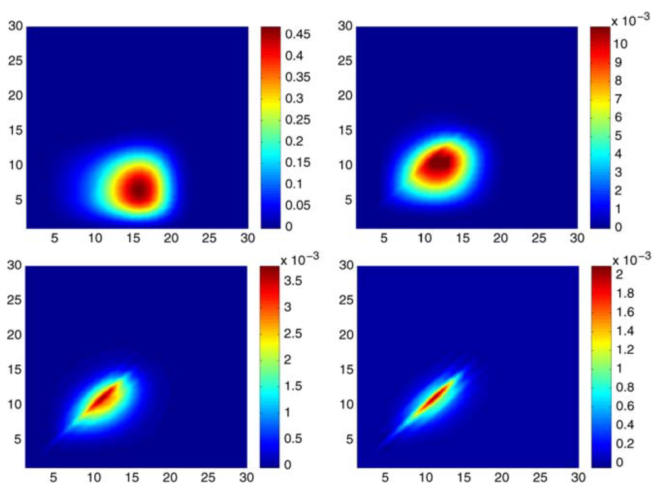
Of interest in 1991 was the performance of the algorithm on parallel vector processors. An accuracy of a micro-Hartree was achieved for the energy. Figure 1 shows the matrix of coefficients for B-spline tensor-product expansions for (or ) pair functions from left to right and top to bottom, respectively. Notice that each subplot has a different scale with the maximum value decreasing. For symmetry, the matrix is approximately the cross-product of the expansion coefficients for the and Hartree–Fock orbitals in a B-spline basis. As l increases, the maximum coefficient (dark red in colour) moves closer to the diagonal region. However more importantly, the significant components are concentrated in a smaller and smaller region. What this calculation clearly shows is that correlation is a “local” correction and that, as the orbital symmetry l increases, an oscillating orthonormal basis would not be an efficient basis.
However the example is also interesting from other perspectives. Like the Hylleraas method, there are no orbitals, nor are there orthonormality constraints and hence, no Lagrange multipliers. The wave function is a sum of pair functions rather than a linear combination of configuration state functions, and there is no matrix diagonalisation. In present grasp [20] or atsp calculations, the usual first step is to compute all angular data, which then needs to be read and stored in memory when needed. With pair functions the amount of angular data is greatly reduced and often could be computed as needed. It should also be remembered that orbitals are a theoretical concept.
5. Spline Galerkin and Inverse Iteration Methods
The development of B-splines (of an order greater than that of cubic splines) began before the LAPACK [21] routines were released. Available instead, were LINPACK [22] routines for solving systems of equations. Some early papers by Froese Fischer and Idrees [23,24], described a spline algorithm for solving the continuum functions that used the spline Galerkin method for deriving linear equations of the form:
and inverse iteration for solving the equation for a given energy. The latter was similar to the power method for finding the eigenvector associated with the largest eigenvalue. For continuum solutions, the energy E is specified and what is needed is the eigenvector of the nearest (or smallest) eigenvalue to E. Like the power method, the method is iterative.
Let the matrix A be an matrix and L and U lower and upper triangular matrices, respectively, of similar dimension, such that . and , is a vector. Then, starting with and incrementing by 1, until the vector c has converged (i.e., ), let:
where x and y are vectors of length N. The method was tested for the hydrogen scattering problem and then photoionisation in He. It was also determined how orthogonality conditions could be included by extending the definition of and the vector c for the case,
as an example. Resonances, phase shifts, or photoionisation cross-sections were extracted from the results. A more extensive investigation of resonance positions and widths for H and He was reported by Brage et al. [25,26], adding to the rich ‘flora’ of results by many different methods for these cases. Xi and Froese Fischer extended these results to three-electron He system in the investigation of cross-section and angular-distribution for the photodetachment of He below the He () threshold [27] and also below the detachment level [28]. A multichannel theory was developed. Among the resonances found was a resonance state immediately below the threshold. A similar theory was applied to Be [29].
6. Spline Methods for Bound State Problems
Several options are available for B-spline solutions that were not feasible for finite difference methods. Consider the simple equation for that was studied by Froese Fischer and Guo [31]. The differential equation that needs to be solved is:
where when or and the radial function is expanded in a B-spline basis so that:
This problem can be linearised by computing from current estimates, and then solved as a generalised eigenvalue problem for an improved estimate, with at best a linear rate of convergence. Or, we can think of the equations as non-linear equations, and solve for changes in the expansion coefficients and energy parameters, using the Newton–Raphson (NR) method with a quadratic rate of convergence (see Ref. [32] for details).
The many-electron variational methods are extensions of the Hartree–Fock methods [3,19] for which three categories of methods have been implemented and evaluated.
6.1. Generalised Eigenvalue Problem for a Single Orbital
In this approach, orbitals are improved one at a time according to a generalized eigenvalue problem,
When two orbitals are constrained through orthogonality, as in the case of , then the iterative process will not converge without first rotating the two orbitals, say a and b for a stationary energy, a process implemented in the sphf program [3]. Projection operators may then be applied to eliminate the off-diagonal Lagrange multiplier The matrix is then a full matrix when exchange contributions are present.
6.2. Multiple Orbitals and SVD
Another possibility is to solve for a set of orbitals at the same time using singular value decomposition (SVD) which is closely related to inverse iteration and is included in LAPACK [21].
Let be the expansion vector for orbital i. Then the system of equations can be written as:
where contains the contributions from one-electron integrals, the direct Slater integrals for orbital i, as well as , and () contains the contribution from exchange integrals between orbitals i and j and possible orthogonality constraints. In this case, all matrices are banded. In this approach, the energy parameters are computed from current estimates of the orbitals.
The earlier SVD study [19] showed poor convergence in the case of but converged linearly. For the latter, the off-diagonal energy parameter is zero and rotation of orbitals is not important. Applying a projection operator to a system of equations is equivalent to using current estimates of a radial function to determine off-diagonal energy parameters. It is possible that SVD equations should be extended to include the energy parameters (diagonal ) as well as off-diagonal () unknowns so that an effective rotation of orbitals is part of the SVD solution.
6.3. Newton–Raphson with Quadratic Rate of Convergence
Consider the case of two orbitals a and b, with an orthogonality constraint between them. Then the unknowns are . The equations to be solved are the two orbital equations along with the three orthonormality conditions that are part of the energy functional. Let be the current estimates that are used to evaluate the -matrix. If symmetry conditions are not satisfied exactly, we can use the average value,
Then, by the Newton–Raphson method [3]. and are solutions of:
In the above, , namely the amount by which the current estimates do not satisfy the equations.
7. The sphf and spmchf Programs
The B-spline methods clearly offer some advantages, even when they are more computationally intensive than finite difference methods. The eigenvalue method is the preferred method for singly occupied orbitals, particularly with large principal quantum numbers. However for a multiply occupied shell, the Newton–Raphson method is efficient in that the “self-energy” is readily accounted for which greatly improves the rate of convergence. When many subshells are present with different principal quantum numbers, convergence can be improved with the simultaneous improvement of orbitals. For this reason, both sphf [3] and spmchf (available at GitHub [33]) have “phases” and different “levels” of accuracy. All iterative methods need initial estimates. The first phase is stable even when estimates are of a poor accuracy and the grid that defines the B-spline basis is relatively coarse. Orbitals are updated sequentially using the generalised eigenvalue method on the first iteration but, in other iterations use NR for a single orbital when a subshell is multiply occupied. This first phase is referred to as the “SCF” phase. The codes also have the initial level of accuracy (with a coarse grid) and less accurate tests for convergence and a higher level of accuracy. When initial estimates are for the refined grid, the program assumes there is only one level of accuracy. In any event, the convergence tests may be reset by the user, over-riding program defaults. Unlike the sphf program, the spmchf program does not include orbital rotation in this phase. The next phase is thought of as a “clean-up” phase that raises the level of accuracy and improves the relationship of one subshell to the other. In the Be case, if the orbital is too contracted the subshell will be too expanded. The NR phase deals with this issue that greatly affects the Virial Theorem (V/T) ratio, as well as orbital rotation when off-diagonal energy parameters are important.
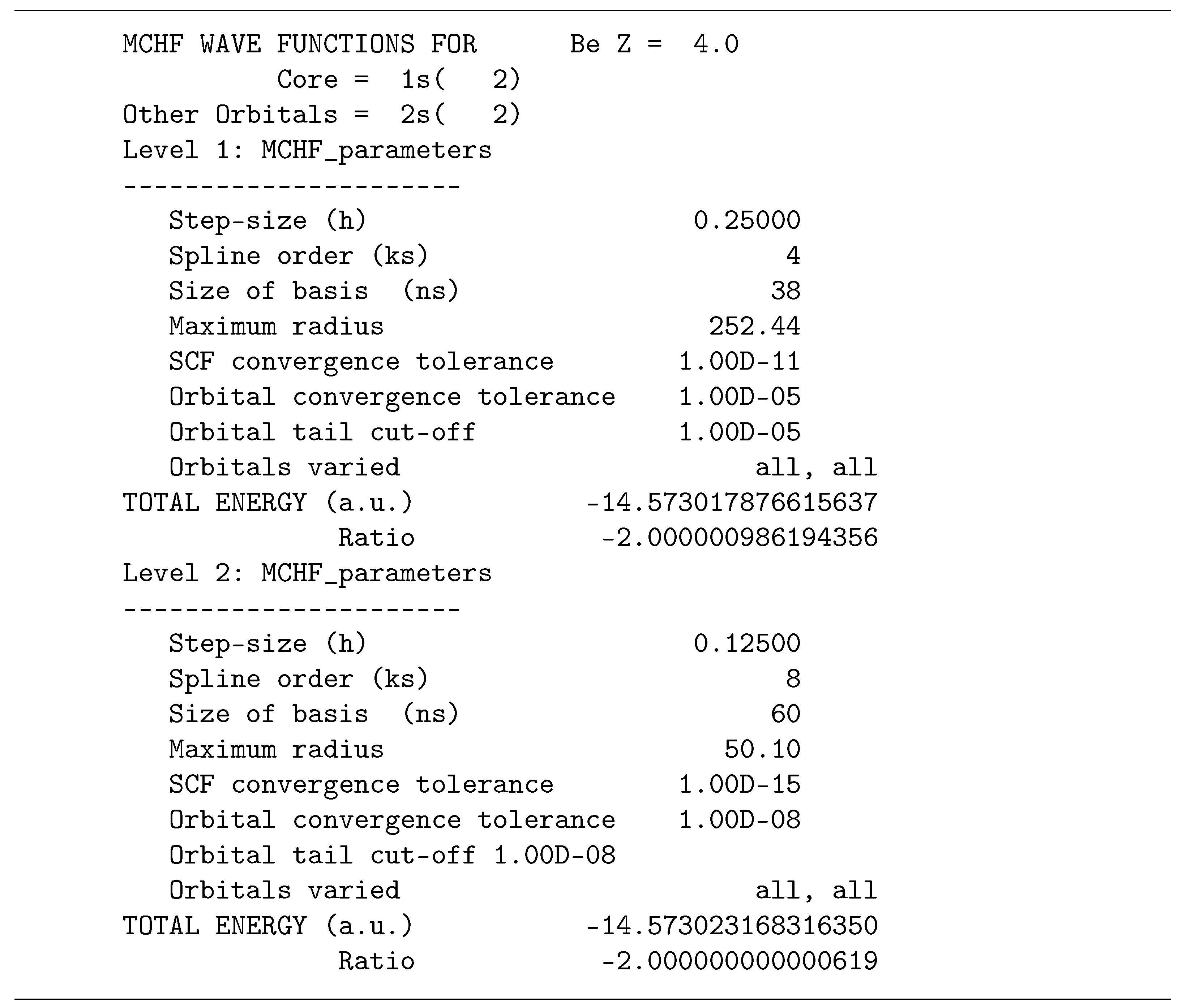
Figure 2 shows the parameters for two levels in the calculation for Be . The default grids and convergence parameters are displayed for both accuracy levels. No initial estimates were provided in this case so the initial range was estimated to be fairly large. At the second level of accuracy, the range is known much more precisely. Notice the improved VT in going from the first to the second level of accuracy. The case is very similar except now off-diagonal Lagrange multipliers are needed for a stationary energy with respect to rotation and the requirement that . Table 1 shows how during the SCF iterations, the values are opposite in sign and the calculations do not converge, but everything changes during the NR iterations and iterations converge rapidly. The default options of dbsr-hf do not include orbital rotations. For the case, it converges but to an incorrect value, made evident only through the Virial theorem (VT). Thus VT is an important check for this code.
The spmchf method differs not only in that expansion coefficients for configuration states (CSFs) need to be determined but also in that the the energy expression is no longer limited to direct () and exchange () Slater integrals. The process by which the energy expression relates to the matrix form requires that two occurrences of the orbital a be present in the matrix element [19]. In the MCHF approximation:
the interaction matrix element is . The spmchf treats the contribution to Equation (27) for or as a “residual” term (not included in the matrix), but Zatsarinny [34] pointed out that if the matrix element was treated as:
then the matrix form could be retained. The factors, and are normalisation integrals. This modification has not yet been implemented in spmchf.
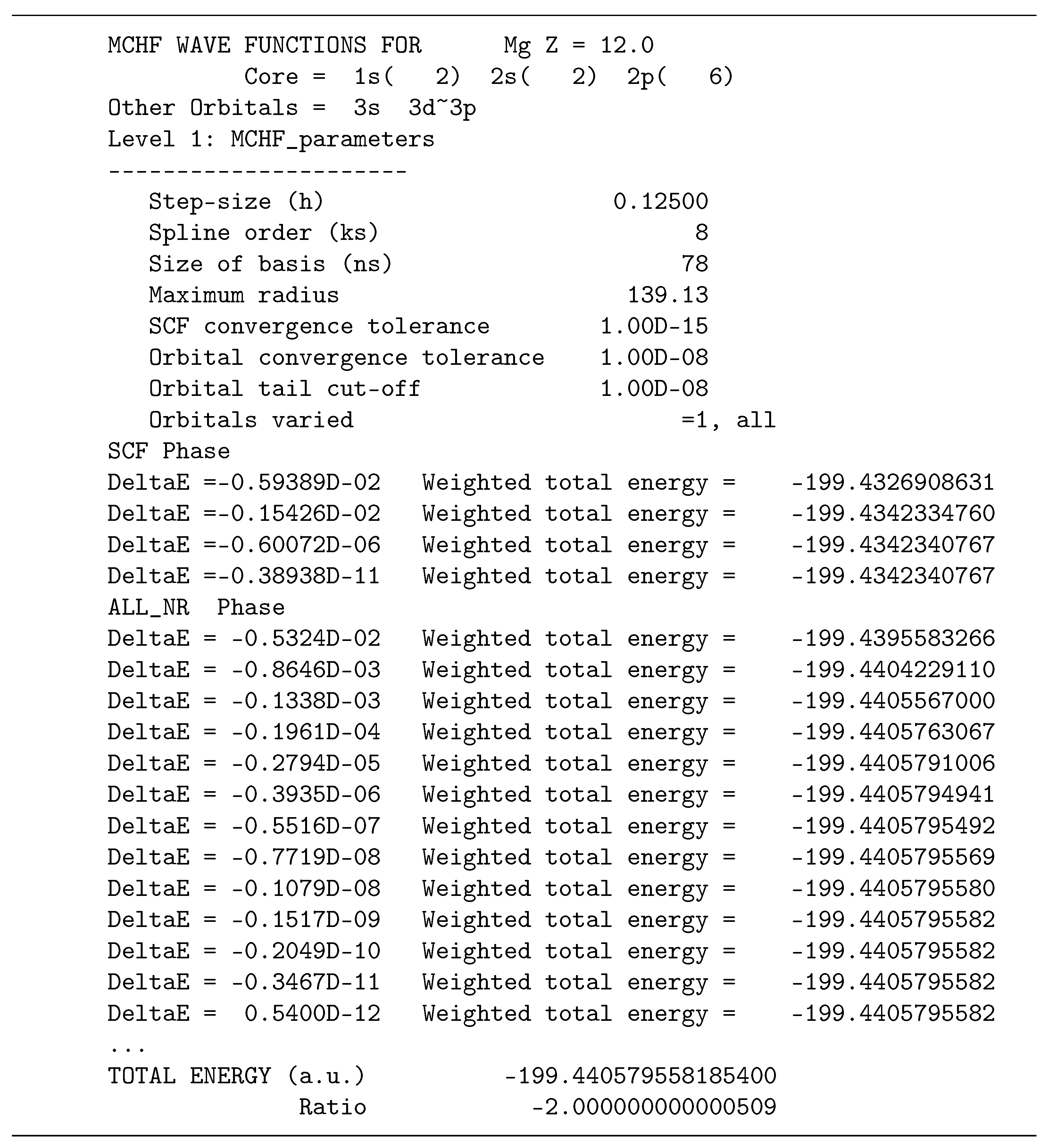
Figure 3 and Figure 4 show the spmchf solution for this example. Neither sphf nor spmchf require initial estimates so the first calculation was for a Hartree Fock calculation for Mg . The output was then used in the second multiconfiguration run as input to serve as initial estimates and the first level varied only the orbital, not present in the input. Then the second varied all orbitals with excellent results as reported.
At this time, the spmchf program for multiconfiguration wave functions has not yet been been fully tested. Through the use of the term=jj command-line option, the fully relativistic dbsr-hf code can be used as an average energy level (EAL) approximation.
8. Concluding Remarks
The spline codes reviewed in this article were developed in the last 20 or so years. For bound state problems, the GRASP code, for example [20], based on finite difference methods and an orthonormal orbital basis, is extensively used for complete spectra including relatively highly excited levels [35] and certain heavy elements, primarily for highly ionised systems where valence correlation can be dealt with and the effect of core correlation on spectra and other properties is limited. spmchf with its greater flexibility still needs to be tested on lanthanides and actinides with two open shells ( for lanthanides and for actinides) where natural orbital transformation could prove useful in connection with orthonormal radial functions [36]. Multiple f-orbitals could also be a challenge for bsr in that the number of determinants can increase rapidly.
In 1984, it took 254 seconds to execute a numerical HF program for Ra on a VAX 11/780; in 1987, 2 seconds on a Cray X-MP; and in 1993, 1 s on a Dec Alpha, which was a popular computer at its time. Thus time (cost) is no longer an important factor but rather ease of use and reliability. The same is not true when accurate wave functions are needed for many-electron systems for different atomic properties. Important now is how well an algorithm can be made parallel, and how efficiently memory usage can be managed.
The present paper has been about non-relativistic calculations. Relativistic methods are similar, except that the decision to represent large and small components of radial functions by splines of different order, automatically implies that every Slater integral is the sum of four integrals. This decision was important in bsr [2] in that it eliminated spurious solutions in the R-matrix and was also used for dbsr-hf. However, is it the most efficient solution of the problem? For a grid of intervals, the number of independent basis functions is . Thus, by going from to , the number of independent basis states decreases. The spurious solutions generally are higher in the spectrum. For bound state solutions, the asymptotic conditions are such that both the large and small components and their derivatives go to zero. In fact, in non-relativistic calculations, applying both conditions stabilises the solution at large r. Further study might be appropriate.
Funding
This research was funded by Canada NSERC Discovery Grant 2017-03851.
Data Availability Statement
Not applicable.
Acknowledgments
Much of the spline research described here was performed over many years at Vanderbilt University with funding support from the Division of Chemical Science, Geosciences, and Bioscience, Office of Basic Energy Sciences, Office of Science, and the U.S. Department of Energy. Some of the program development was performed while at the Atomic Physics Division, National Institute of Standards and Technology, Gaithersburg, and Maryland 20899-8422. The author very much appreciated Professor Michel R. Godefroid’s comments and suggestions for this paper.
Conflicts of Interest
The author declares no conflict of interest.
References
- Zatsarinny, O. A general program for computing matrix elements for atomic structure with nonorthogonal orbitals. Comp. Phys. Commun. 1996, 98, 235–254. [Google Scholar] [CrossRef]
- Zatsarinny, O. BSR: B-spline atomic R-matrix codes. Comput. Phys. Commun. 2006, 174, 273–356. [Google Scholar] [CrossRef]
- Froese Fischer, C. A B-spline Hartree-Fock program. Comput. Phys. Commun. 2011, 182, 1315–1326. [Google Scholar]
- Igarashi, A. B-Spline Expansions in Radial Dirac Equation. J. Phys. Soc. Jpn. 2006, 75, 114301. [Google Scholar] [CrossRef]
- Igarashi, A. Kinetically balanced B-spline expansions in radial Dirac equation. J. Phys. Soc. Jpn. 2007, 76, 05431. [Google Scholar] [CrossRef]
- Froese Fischer, C.; Zatsarinny, O. A B-spline Galerkin method for the Dirac equation. Comput. Phys. Commun. 2009, 180, 879–886. [Google Scholar] [CrossRef] [Green Version]
- Zatsarinny, O.; Froese Fischer, C. DBSR—A B-spline Dirac-Hartree-Fock program. Comput. Phys. Commun. 2016, 202, 287–303. [Google Scholar] [CrossRef] [Green Version]
- Hartree, D.R. The Calculations of Atomic Structures; Springer: New York, NY, USA, 1957. [Google Scholar]
- Roothaan, C.C.J. New Developments in Molecular Orbital Theory. Rev. Mod. Phys. 1951, 23, 69–89. [Google Scholar] [CrossRef]
- Bachau, H.; Cormier, E.; Decleva, P.; Hansen, J.E.; Martin, F. Applications of B-splines in atomic and molecular physics. Rep. Prog. Phys. 2001, 64, 1815–1942. [Google Scholar] [CrossRef]
- de Boor, C. A Practice Guide to Splines; Springer: New York, NY, USA, 1985. [Google Scholar]
- Johnson, W.R.; Sapirstein, J. Computation of Second-Order Many-Body Corrections in Relativistic Atomic Systems. Phys. Rev. Lett. 1986, 57, 1126. [Google Scholar] [CrossRef]
- Froese Fischer, C. A general multiconfiguration Hartree-Fock program. Comput. Phys. Commun. 1978, 14, 145–153. [Google Scholar] [CrossRef]
- Froese Fischer, C.; Tachiev, G.; Gaigalas, G.; Godefroid, M.R. An MCHF atomic-structure package for large-scale calculations. Comput. Phys. Commun. 2007, 176, 559–579. [Google Scholar] [CrossRef] [Green Version]
- Hibbert, A.; Froese Fischer, C.; Godefroid, M.R. Non-orthogonal orbitals in MCHF or configuration interaction wave functions. Comput. Phys. Commun. 1988, 51, 282–293. [Google Scholar] [CrossRef]
- Froese Fischer, C.; Parpia, F.A. Accurate spline solutions of the radial Dirac equation. Phys. Lett. A 1993, 179, 198–204. [Google Scholar] [CrossRef]
- Qiu, Y.; Froese Fischer, C. Integration by cell algorithm for Slater integrals in a spline basis. J. Comput. Phys. 1999, 156, 257–271. [Google Scholar] [CrossRef]
- Froese Fischer, C. Concurrent vector algorithms for spline solutions of the helium pair equation. Int. J. High Perform. Comput. Appl. 1991, 5, 5–20. [Google Scholar] [CrossRef]
- Froese Fischer, C. B-splines in variational atomic structur calculations. Adv. At. Mol. Phys. 2007, 55, 539–550. [Google Scholar]
- Froese Fischer, C.; Gaigalas, G.; Jönsson, P.; Bieroń, J. GRASP2018—A Fortran 95 version of the General Relativistic Atomic Structure Package. Comput. Phys. Commun. 2019, 237, 184–187. [Google Scholar] [CrossRef]
- LAPACK Library. Available online: http://www.netlib.org/lapack/ (accessed on 28 July 2021).
- LINPACK Library. Available online: http://www.netlib.org/linpack/ (accessed on 28 July 2021).
- Froese Fischer, C.; Idrees, M. Spline algorithms for continuum functions. Comput. Phys. 1989, 3, 53–58. [Google Scholar] [CrossRef]
- Froese Fischer, C.; Idrees, M. Spline methods for resonances in photoionisation cross sections. J. Phys. B At. Mol. Opt. Phys. 1990, 23, 679. [Google Scholar] [CrossRef]
- Brage, T.; Froese Fischer, C.; Miecznik, G. Non-variational, spline-Galerkin calculations of resonance positions and widths, and photodetachment and photoionization cross sections for H− and He. J. Phys. B At. Mol. Opt. Phys. 1992, 25, 5289–5314. [Google Scholar] [CrossRef]
- Brage, T.; Froese Fischer, C. Spline-Galerkin methods for Rydberg series, including Breit-Pauli effects. J. Phys. B At. Mol. Opt. Phys. 1994, 27, 5467–5484. [Google Scholar] [CrossRef]
- Xi, J.; Froese Fischer, C. Cross section and angular distribution for the photodetachment of He−1s2s2p4Po below the He n = 4 threshold. Phys. Rev. A 1996, 53, 3169–3177. [Google Scholar] [CrossRef]
- Xi, J.; Froese Fischer, C. Photodetachment cross-section of He- (1s2s2p4Po ) in the region of the 1s detachment threshold. Phys. Rev. A 1999, 59, 307–314. [Google Scholar] [CrossRef]
- Xi, J.; Froese Fischer, C. Cross section and angular distribution for photodetachment of Be− 1s22s2p24P. J. Phys. B At. Mol. Opt. Phys. 1999, 32, 387–396. [Google Scholar] [CrossRef]
- Zatsarinny, O.; Froese Fischer, C. The use of basis splines and non-orthogonal orbitals in R-matrix calculations: Application to Li photoionization. J. Phys. B At. Mol. Opt. Phys. 2000, 33, 313–341. [Google Scholar] [CrossRef]
- Froese Fischer, C.; Guo, W. Spline algorithms for the Hartree-Fock equation for the helium ground state. J. Comput. Phys. 1990, 90, 486–496. [Google Scholar] [CrossRef]
- Froese Fischer, C.; Guo, W.; Shen, Z. Spline methods for multiconfiguration Hartree-Fock calculations. Int. J. Quantum Chem. 1992, 42, 849–867. [Google Scholar] [CrossRef]
- spmchf. Available online: http://github.com/compas/spmchf (accessed on 28 July 2021).
- Zatsarinny, O.; Drake Umiversity. Private communication, 1 May 2016.
- Li, W.; Amarsi, A.M.; Papoulia, A.; Ekman, J.; Jönsson, P. Extended theoretical transition data in C i–iv. Mon. Not. R. Astron. Soc. 2021, 502, 3780–3799. [Google Scholar] [CrossRef]
- Schiffmann, S.; Godefroid, M.; Ekman, J.; Jönsson, P.; Froese Fischer, C. Natural orbitals in multiconfiguration calculations of hyperfine-structure parameters. Phys. Rev. A 2020, 101, 062510. [Google Scholar] [CrossRef]
Figure 1.
A visualisation of the magnitude of the matrix of expansion coefficients for the state of Helium. Shown, from left to right and top to bottom, are the expansion coefficients for the , , , and pair functions. The maximum values are 0.45, 0.010, 0.0035, 0.0020, respectively. Note both the changing region and decreasing maximum magnitude of each partial wave. (See also [19].)

Figure 2.
Computer output showing the convergence for the two levels of accuracy. The calculations are for Be .
Figure 2.
Computer output showing the convergence for the two levels of accuracy. The calculations are for Be .

Figure 3.
Computer output of a Hartree–Fock calculation for the Mg [Ne] wave function.

Figure 4.
Computer output for multiconfiguration calculation for . Calculations are for Mg [Ne] using the radial functions from Figure 3 as initial estimates.
Figure 4.
Computer output for multiconfiguration calculation for . Calculations are for Mg [Ne] using the radial functions from Figure 3 as initial estimates.


Table 1.
Table showing the convergence of off-diagonal energy parameters and as a function of the iteration (i) for the eigenvalue SCF iteration updating orbitals sequentially and the Newton–Raphson (NR) method updating both simultaneously. The calculations are for He . The values for of the SCF iteration are computed from initial estimates. For all other iterations, values are determined after the iteration has completed. For exact solutions, . Note that the SCF process did not converge.
| SCF | NR | ||||
|---|---|---|---|---|---|
| i | i | ||||
| 0 | 0.03432768 | 0.35742083 | 4 | 0.15038917 | 0.14949971 |
| 1 | −0.00696379 | 0.13503646 | 5 | 0.15093334 | 0.15089696 |
| 2 | −0.00969413 | 0.14106384 | 6 | 0.15089696 | 0.15089696 |
| 3 | −0.00968723 | 0.14104181 | 7 | 0.15089691 | 0.15089691 |
| 8 | 0.15089706 | 0.15089705 | |||
Publisher’s Note: MDPI stays neutral with regard to jurisdictional claims in published maps and institutional affiliations. |
© 2021 by the author. Licensee MDPI, Basel, Switzerland. This article is an open access article distributed under the terms and conditions of the Creative Commons Attribution (CC BY) license (https://creativecommons.org/licenses/by/4.0/).
Share and Cite
MDPI and ACS Style
Fischer, C.F. Towards B-Spline Atomic Structure Calculations. Atoms 2021, 9, 50. https://0-doi-org.brum.beds.ac.uk/10.3390/atoms9030050
AMA Style
Fischer CF. Towards B-Spline Atomic Structure Calculations. Atoms. 2021; 9(3):50. https://0-doi-org.brum.beds.ac.uk/10.3390/atoms9030050
Chicago/Turabian StyleFischer, Charlotte Froese. 2021. "Towards B-Spline Atomic Structure Calculations" Atoms 9, no. 3: 50. https://0-doi-org.brum.beds.ac.uk/10.3390/atoms9030050
Note that from the first issue of 2016, this journal uses article numbers instead of page numbers. See further details here.