Redistribution of the Rydberg State Population Induced by Continuous-Spectrum Radiation

Abstract

We consider the redistribution of the Rydberg state population resulting from multistep cascade transitions induced by radiation with a continuous spectrum. The population distribution is analyzed within the space of quantum numbers n and l. The dynamics of the system are studied using both the numerical solution of kinetic equations and the diffusion approximation based on the Fokker–Planck equation. The main path of the redistribution process is determined.

1. Introduction

Interest in the diffusion-like redistribution of the Rydberg state population induced by radiation has been aroused by experimental observation of microwave ionization of hydrogen Rydberg states [1,2,3]. This process has been described within the framework of classical chaotic motion theory [4,5,6,7,8] or, alternatively, in terms of quantum diffusion [9]. This description of the process has accordingly been termed “diffusion ionization” (alternative terms are “stochastic“ or “diffusive” ionization).

Diffusion ionization occurs when an incident radiation photon has insufficient energy to induce photoionization from the initial state. The mechanism of diffusion ionization can be described as follows: multistep cascade transitions translate an atomic electron to a highly excited state from which an electron ionizes. This mechanism is referred to as diffusion ionization because multistep transitions can be effectively described as the diffusion of the population in energy space.

In the present study, we focus on the first stage of the described process, i.e., the diffusive redistribution of the Rydberg state population induced by radiation.

The earlier studies on this process [4,5,6,7,8,9] considered the case of monochromatic radiation in line with the experimental conditions [1]. In this case, the radiation should be sufficiently strong to induce significant Stark splitting [9] and broadening [10] of atomic levels, because it was necessary to provide a sufficient number of transitions in the atomic spectrum with the same frequency as that of the incident radiation.

In the present study, we consider radiation with a continuous spectrum. Thus, a strong perturbation of the atomic spectrum is not necessary to produce multistep transitions, which can instead be induced by less intense radiation. In general, the study of continuous-spectrum radiation effect on Rydberg states began more than four decades ago with the pioneering work by Gallagher and Cooke [11] and continued in many experimental and theoretical works concerning interaction of the Rydberg states with the blackbody radiation, for example [12,13,14,15]. However, long multistep transitions in this case have been much less studied than in the monochromatic radiation case. The results of experimental studies [16] have shown the significant impact of cascade processes on the ionization probability, but these processes have not been systematically investigated. Preliminary estimates of the diffusion ionization of the Rydberg states induced by blackbody radiation were provided in [17] but there were no continuations. Galvez et al. [18] investigated cascade transitions between Rydberg states of Na induced by blackbody radiation, but they considered mainly two- and three-step transitions. Furthermore, Beterov et al. experimentally measured the ionization rate of the Rydberg states of alkali metals induced by blackbody radiation [19] and performed corresponding theoretical calculations [20,21,22] taking cascade processes into account; however, the number of steps in the considered cascades again did not exceed four.

Multistep cascade processes can play an important role in some astrophysical applications. In particular, these processes can contribute to non-LTE (NLTE, LTE: Local Thermodynamical Equilibrium) corrections to the population distribution for thin stellar atmospheres and nebulae. Generally, statistical balance equations are to be solved to compute these corrections. However, a high number of steps in the cascade drastically increases the number of states included in these equations [23]. This problem can be solved by using the Fokker–Planck equation to transform the discrete representation of the process to a continuous representation, which is the diffusion approximation. A similar approach is actively used to describe collisional processes [24,25,26,27,28] but is less developed for radiative ones.

Our previous work [29] focused on the diffusion ionization of the sodium atom induced by continuous-spectrum radiation. The redistribution of the population was analyzed using both kinetic equations and the Fokker–Planck equation. The numerical solution to the kinetic equations confirmed the validity of the diffusion approximation. However, the population for sodium mostly only spread within s- and p-states because of the large quantum defects of these states. The similar effect was experimentally obtained for sodium in [30].

In the present study, the redistribution of the population is considered within the space of quantum numbers n and l of the hydrogen atom. In Section 2, the case of incident radiation with a rectangular spectrum is considered, and the results for an arbitrary continuous spectrum are presented in Section 3.

Atomic units are used throughout. In particular, for the time the atomic unit is approximately equal to $2.419\times {10}^{-17}\mathrm{s}$, and correspondingly, for the angular frequency $\omega$ it is approximately $4.134\times {10}^{16}\mathrm{rad}/\mathrm{s}$.

2. Diffusion throughout States Induced by Radiation with a Rectangular Spectrum

The radiation is assumed to be stochastic, whereby the kinetic equations can be used to describe the electron transitions

$$\frac{d{N}_{nl}}{dt}=\sum _{n^{\prime }{l}^{\prime }}V(n^{\prime }{l}^{\prime }\to nl)N_{n^{\prime }{l}^{\prime }}-N_{nl}\left(\sum _{n^{\prime }{l}^{\prime }}V(nl\to n^{\prime }{l}^{\prime })+W_i\left(nl\right)\right).$$

(1)

Here, $N_{nl}$ is the population of the state ($nl$), i.e., the occupation number of the state ($nl$). $N_{nl}$ is equal to 0 if the state ($nl$) is not populated and is equal to 1 if it is completely populated. $V(nl\to n^{\prime }{l}^{\prime })$ is the rate of the transition $nl\to n^{\prime }{l}^{\prime }$ equal to the sum of rates of induced and spontaneous transitions

$$V(nl\to n^{\prime }{l}^{\prime })=V_{\mathrm{ind}}(nl\to n^{\prime }{l}^{\prime })+V_{\mathrm{sp}}(nl\to n^{\prime }{l}^{\prime }).$$

$W_i\left(nl\right)$ is the rate of the photoionization. The initial state of the electron is denoted by $(n_0,l_0)$.

In this section, the spectral density $\rho \left(\omega \right)$ of the incident radiation is assumed to be distributed in a limited frequency range between the boundary values of the frequencies ${\omega }_{min}$ and ${\omega }_{max}$, i.e., $\rho \left(\omega \right)=0$ for $\omega <{\omega }_{min}$ or $\omega >{\omega }_{max}$. For certainty, we also assume $\rho \left(\omega \right)$ to be constant in this range, i.e., $\rho \left(\omega \right)=\rho =\mathrm{const}$ for ${\omega }_{min}\le \omega \le {\omega }_{max}$. In other words, we consider in this section the case of the radiation with a rectangular spectrum. It is an abstract one and is taken here to simplify the qualitative analysis and show general features of the population redistribution process. Specific values of ${\omega }_{min}$, ${\omega }_{max}$ and $\rho$ used in the simulation do not represent the spectrum of any real source and are chosen so that to get a clear visual representation of the process. (In Section 3 we generalize the analysis and consider the effect of the radiation with arbitrary spectrum.)

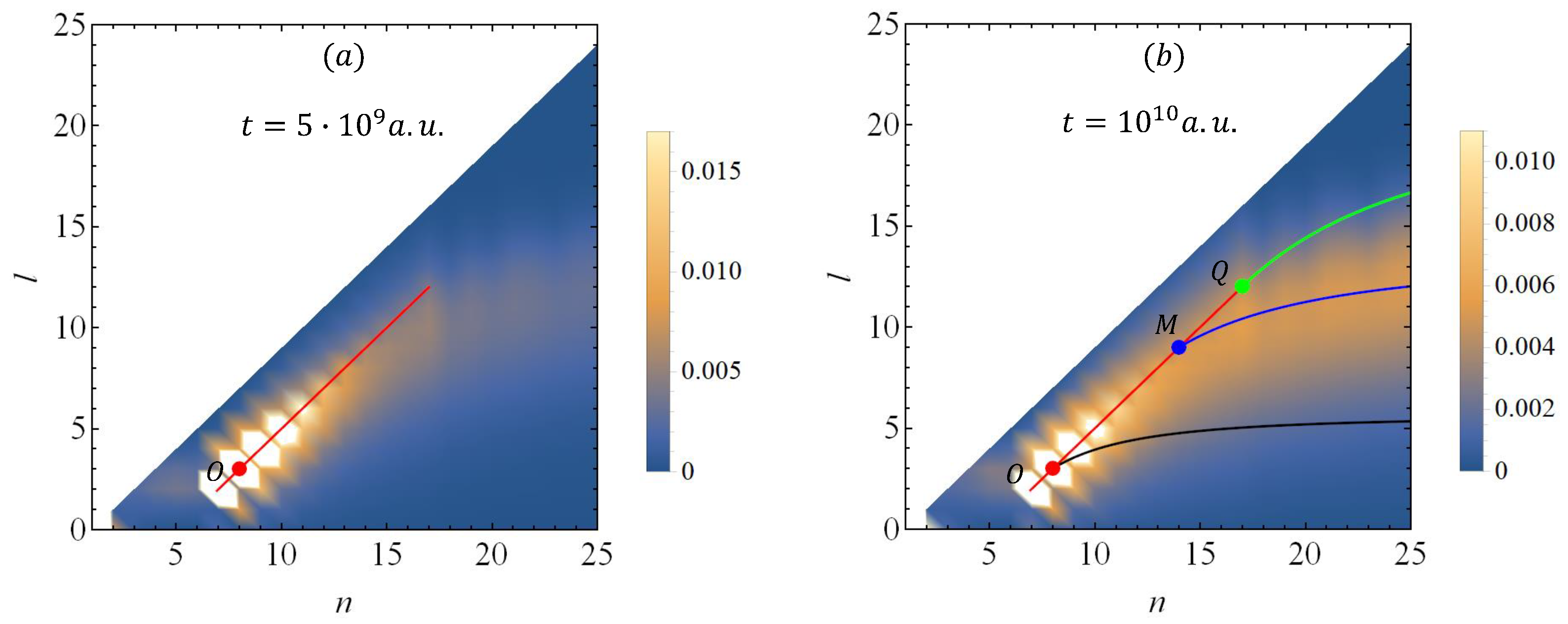
The system is simulated by numerically solving the kinetic Equation (1). Figure 1 shows the simulated distribution of the population in coordinates $n,l$ at two particular moments in time. In line with the simulations results, two main stages in the dynamics of the population redistribution can be identified:

• Figure 1a: The population propagates along the straight (red) line.
• Figure 1b: The population spreads over a region approximately constrained by well-defined boundaries (red, green and black lines). The form of these boundaries is discussed below.

2.1. The Boundaries of the Population Distribution Region

Incident radiation with a frequency $\omega$ induces a dipole transition with the following changes in the energy and orbital moment:

$$\mathsf{\Delta }E=\pm \omega ,\mathsf{\Delta }l=\pm 1.$$

(2)

Considering the Bethe rule [31], the most likely transitions have the same signs of $\mathsf{\Delta }E$ and $\mathsf{\Delta }l$, i.e., if $\mathsf{\Delta }E=\omega$, then $\mathsf{\Delta }l=1$, and if $\mathsf{\Delta }E=-\omega$, then $\mathsf{\Delta }l=-1$. That is, these transitions occur for $\mathsf{\Delta }E/\mathsf{\Delta }l=\omega$. Hence, if the radiation has a continuous spectrum and contains frequencies in the range ${\omega }_{min}\le \omega \le {\omega }_{max}$, then

$${\omega }_{min}\le \frac{\mathsf{\Delta }E}{\mathsf{\Delta }l}\le {\omega }_{max}.$$

(3)

Thus, if only the transitions satisfying the Bethe rule are considered, then the population does not redistribute throughout all states but only those within the boundaries defined by the inequality (3).

The right side of (3) corresponds to transitions with frequencies $\omega ={\omega }_{max}$ and $\mathsf{\Delta }l=1$. The cascade of these transitions from the initial state defines the path satisfying the following equation:

$$l=\frac{1}{{\omega }_{max}}(E-E_0)+l_0.$$

(4)

Taking into account $E=-1/2n^2$, the equation can be written in coordinates $n,l$ as follows:

$$l=\frac{1}{{\omega }_{max}}\left(-\frac{1}{2n^2}+\frac{1}{2n_0^2}\right)+l_0.$$

(5)

This path is the lower boundary of the population distribution region. This boundary is shown by a black line in Figure 1b.

Now, let us consider the left part of (3). It can be refined in the following way. The frequency of the induced transition cannot be lower than the difference of energies between the adjacent levels ${\omega }_n=E_{n+1}-E_n$. Accordingly, if ${\omega }_n$ exceeds ${\omega }_{min}$, ${\omega }_n$ replaces ${\omega }_{min}$ in (3). As a result, the upper boundary in Figure 1b is composite. The upper boundary consists of a segment for ${\omega }_n>{\omega }_{min}$, which is shown as a red line, and a segment for ${\omega }_n<{\omega }_{min}$, which is shown as a green line. The intersection of the two segments is denoted by the point Q. At this point, ${\omega }_n\approx {\omega }_{min}$. An approximate estimate for the corresponding value of the principal quantum number is given below.

$$n_Q={\omega }_{min}^{-1/3}$$

(6)

The red line corresponds to the path along which $\omega ={\omega }_n$, i.e., the cascade of transitions with $\mathsf{\Delta }n=1$. The corresponding equation is

$$l=n-n_0+l_0.$$

(7)

This equation can be used to obtain an explicit formula for $l_Q$:

$$l_Q=n_Q-n_0+l_0.$$

(8)

The green line indicates the cascade of transitions with $\omega ={\omega }_{min}$ from the state ($n_Q,l_Q$). The corresponding equation can be written as

$$l=\frac{1}{{\omega }_{min}}\left(-\frac{1}{2n^2}+\frac{1}{2n_Q^2}\right)+l_Q.$$

(9)

As previously mentioned, this analysis is simplified. As the Bethe rule is not strict, states outside the described boundaries may also be populated. However, as the simulation shows, the majority of the population is located within the described boundaries.

Furthermore, Figure 1b shows that the population does not propagate uniformly within these boundaries. The population mostly propagates along a main path. Initially, the population spreads along the red line shown in Figure 1b. The population then deflects from the red line at the point denoted by M and spreads along the blue line. The segment $OM$ and the blue line are then collectively referred to as the “main path”. This path is discussed in the following section. To determine the location of the path precisely, a more sophisticated analysis using the diffusion approximation is needed. This analysis is presented below.

2.2. The Main Path

According to [24,32], the Fokker–Planck equation is obtained from (1) (see Appendix A):

$$\frac{\partial N}{\partial t}=-\frac{\partial }{\partial n}{A}_{n}N-\frac{\partial }{\partial l}{A}_{l}N+\frac{{\partial }^2}{\partial n^2}{B}_{nn}N+2\frac{{\partial }^2}{\partial n\partial l}{B}_{nl}N+\frac{{\partial }^2}{\partial l^2}{B}_{ll}N-(W_i+W_q)N,$$

(10)

where the coefficients of drift A and diffusion B are defined as follows:

$$\begin{array}{c}\hfill A_n=\sum _{n^{\prime }{l}^{\prime }}{V}_{\mathrm{ind}}(nl\to n^{\prime }{l}^{\prime })(n^{\prime }-n),\end{array}$$

(11)

$$\begin{array}{c}\hfill A_l=\sum _{n^{\prime }{l}^{\prime }}{V}_{\mathrm{ind}}(nl\to n^{\prime }{l}^{\prime })(l^{\prime }-l),\end{array}$$

(12)

$$\begin{array}{c}\hfill B_{nn}=\frac{1}{2}\sum _{n^{\prime }{l}^{\prime }}{V}_{\mathrm{ind}}(nl\to n^{\prime }{l}^{\prime }){(n^{\prime }-n)}^2,\end{array}$$

(13)

$$\begin{array}{c}\hfill B_{nl}=\frac{1}{2}\sum _{n^{\prime }{l}^{\prime }}{V}_{\mathrm{ind}}(nl\to n^{\prime }{l}^{\prime })(n^{\prime }-n)(l^{\prime }-l),\end{array}$$

(14)

$$\begin{array}{c}\hfill B_{ll}=\frac{1}{2}\sum _{n^{\prime }{l}^{\prime }}{V}_{\mathrm{ind}}(nl\to n^{\prime }{l}^{\prime }){(l^{\prime }-l)}^2,\end{array}$$

(15)

and $W_q$ is the rate of spontaneous decay

$$W_q=\sum _{n^{\prime }{l}^{\prime }}{V}_{\mathrm{sp}}(nl\to n^{\prime }{l}^{\prime }).$$

(16)

Speaking simplistically, the drift terms in (10) correspond to the population transfer due to asymmetry of the probabilities $V_{\mathrm{ind}}(nl\to n^{\prime }{l}^{\prime })$: if $V_{\mathrm{ind}}(nl\to n+\mathsf{\Delta }n,l+\mathsf{\Delta }l)\gg V_{\mathrm{ind}}(nl\to n-\mathsf{\Delta }n,l-\mathsf{\Delta }l)$ then the population moves in the direction $(\mathsf{\Delta }n,\mathsf{\Delta }l)$. On the other hand, the diffusion terms in (10) correspond to the population transfer due to unevenness of the population distribution: if $N_{nl}\gg N_{n^{\prime }{l}^{\prime }}$ then $N_{nl}$ decreases and $N_{n^{\prime }{l}^{\prime }}$ rises.

Numerical simulation of the kinetic equation shows that the redistribution of Rydberg state population is determined mainly by the diffusion terms: the drift terms are much smaller than the diffusion ones, and the photoionization and the spontaneous decay cause the population depletion of all the Rydberg states in general, so they do not change the main path of the process. Thus, further we consider the reduced version of the Fokker–Planck Equation (10):

$$\frac{\partial N}{\partial t}=\frac{{\partial }^2}{\partial n^2}{B}_{nn}N+2\frac{{\partial }^2}{\partial n\partial l}{B}_{nl}N+\frac{{\partial }^2}{\partial l^2}{B}_{ll}N.$$

(17)

Let us consider an auxiliary Cauchy problem for (17). Let at a moment t all population located at an arbitrary state $(n,l)$, not necessarily $(n_0,l_0)$, and try to find the population at some $(n^{\prime },l^{\prime })$ for $t^{\prime }>t$. If $\mathsf{\Delta }t=t^{\prime }-t$ is sufficiently small, then the coefficients $B_{nn}$, $B_{ll}$, $B_{nl}$ can be assumed approximately constant, and this auxiliary problem has solution

$$N\sim exp\left[-\frac{1}{4\mathsf{\Delta }t}\left(\frac{B_{ll}\mathsf{\Delta }{n}^2+2B_{nl}\mathsf{\Delta }n\mathsf{\Delta }l+B_{nn}\mathsf{\Delta }{l}^2}{B_{nn}{B}_{ll}-B_{nl}^2}\right)\right],$$

where $\mathsf{\Delta }n=n^{\prime }-n$, $\mathsf{\Delta }l=l^{\prime }-l$.

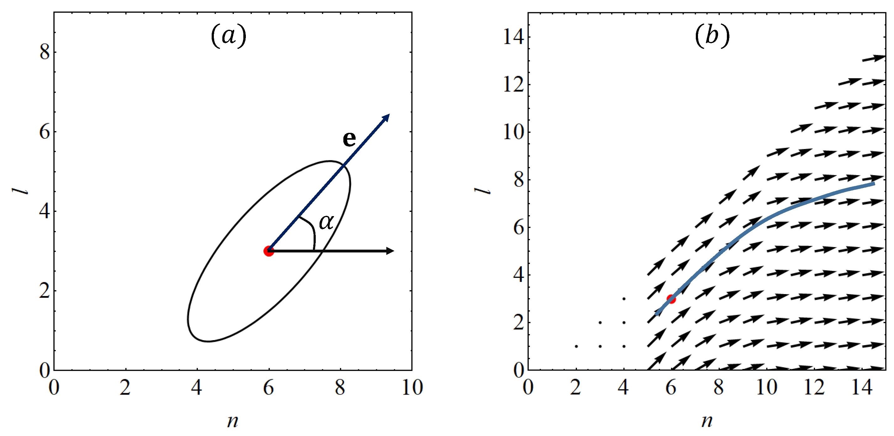
The corresponding diffusion front (the set of all points with the same exponent) is elliptical:

$$B_{ll}\mathsf{\Delta }{n}^2+2B_{nl}\mathsf{\Delta }n\mathsf{\Delta }l+B_{nn}\mathsf{\Delta }{l}^2=4\mathsf{\Delta }t(B_{nn}{B}_{ll}-B_{nl}^2).$$

and is hereafter referred to as the local diffusion ellipse (Figure 2a). Hence, the diffusion in a sufficiently small environment of $(n,l)$ will mainly occur along the main axis of this ellipse. In other words, if at a some moment of time the electron arrives in a state $(n,l)$, then in a next moment it will most probably go along this main axis. This direction is given by

$$cot\alpha =\frac{B_{nn}-B_{ll}+\sqrt{{(B_{ll}-B_{nn})}^2+4B_{nl}^2}}{2B_{nl}}.$$

(18)

Accordingly, this direction at each point of the plane $n,l$ defines the vector field of the population flow (see Figure 2b), i.e., the population mainly propagates along this vector field streamlines, which are determined by the equation

$$\frac{dn}{dl}=cot\alpha .$$

(19)

Hence, the main path presented in the previous section is the streamline passing through the point ($n_0,l_0$).

Let us review the form of the main path. For the initial segment OM of the path, $cot\alpha \approx 1$. Taking into account (18), this expression is equivalent to the relation between the diffusion coefficients:

$$B_{nn}-B_{ll}\ll B_{nl}$$

(20)

However, $B_{nn}-B_{ll}$ increases with n. As a result, the main path deflects from the red line at point M. Thus, the relation

$$B_{nn}-B_{ll}\approx B_{nl}$$

(21)

can be used to define the deflection point M. In order to obtain the $(n,l)$-coordinates of the point M explicitly, consider the expressions for the diffusion coefficients in details.

Considering the Bethe rule and assuming transitions occur at a similar rate in the directions of both increasing and decreasing l, the diffusion coefficients (13)–(15) can be recast as follows:

$$\begin{array}{cc}\hfill B_{nn}& {\displaystyle \approx \sum _{\mathsf{\Delta }{n}_{min}}^{\mathsf{\Delta }{n}_{max}}{V}_{\mathrm{ind}}(nl\to n+\mathsf{\Delta }n,l+1)\mathsf{\Delta }{n}^2,}\end{array}$$

(22)

$$\begin{array}{cc}\hfill B_{nl}& {\displaystyle \approx \sum _{\mathsf{\Delta }{n}_{min}}^{\mathsf{\Delta }{n}_{max}}{V}_{\mathrm{ind}}(nl\to n+\mathsf{\Delta }n,l+1)\mathsf{\Delta }n,}\end{array}$$

(23)

$$\begin{array}{cc}\hfill B_{ll}& {\displaystyle \approx \sum _{\mathsf{\Delta }{n}_{min}}^{\mathsf{\Delta }{n}_{max}}{V}_{\mathrm{ind}}(nl\to n+\mathsf{\Delta }n,l+1).}\end{array}$$

(24)

Here,

$$\begin{array}{cc}& \mathsf{\Delta }{n}_{min}\approx max(1,{\omega }_{min}{n}^3),\end{array}$$

(25)

$$\begin{array}{cc}& \mathsf{\Delta }{n}_{max}\approx {\omega }_{max}{n}^3\end{array}$$

(26)

correspond to the minimal and maximal changes in n, respectively, that are allowed for.

To calculate the sums (22)–(24), it is necessary to know the form of the dependence of $V_{\mathrm{ind}}(nl\to n+\mathsf{\Delta }n,l+1)$ on $\mathsf{\Delta }n$. This form can be obtained using the quasiclassical approximation assuming $n,l\gg \mathsf{\Delta }n$ [33]:

$$V_{\mathrm{ind}}(nl\to n+\mathsf{\Delta }n,l+1)=\rho f(n,l){\left(\frac{n^{\prime }n}{n^2-{n^{\prime }}^2}\right)}^3\approx \frac{1}{8}\rho f(n,l){\left(\frac{n}{\mathsf{\Delta }n}\right)}^3,$$

(27)

where $f(n,l)$ is a slowly varying function of n and l given in [33].

Substituting (27) into (22)–(24) enables the diffusion coefficients to be expressed as the sums of harmonic series:

$$\begin{array}{cc}\hfill B_{nn}& {\displaystyle \approx f(n,l)n^3\rho \sum _{\mathsf{\Delta }{n}_{min}}^{\mathsf{\Delta }{n}_{max}}\frac{1}{\mathsf{\Delta }n},}\end{array}$$

(28)

$$\begin{array}{cc}\hfill B_{nl}& {\displaystyle \approx f(n,l)n^3\rho \sum _{\mathsf{\Delta }{n}_{min}}^{\mathsf{\Delta }{n}_{max}}\frac{1}{\mathsf{\Delta }{n}^2},}\end{array}$$

(29)

$$\begin{array}{cc}\hfill B_{ll}& {\displaystyle \approx f(n,l)n^3\rho \sum _{\mathsf{\Delta }{n}_{min}}^{\mathsf{\Delta }{n}_{max}}\frac{1}{\mathsf{\Delta }{n}^3}.}\end{array}$$

(30)

Using the Euler–Maclaurin formula to estimate the sums (28)–(30) and substituting (25) and (26) into these sums yields an explicit formula for the principal quantum number of the point M from the condition (21):

$$n_M\approx min\left[{\omega }_{min}^{-1/3},{\left(\xi {\omega }_{max}\right)}^{-1/3}\right],$$

(31)

where $\xi ={[exp(\frac{{\pi }^2}{6}-\gamma +{\zeta }_3)]}^{-1}\approx 0.1$. Here, $\gamma \approx 0.58$ is the Euler constant, and ${\zeta }_3\approx 1.2$ is the Apéry constant.

Accordingly, if ${\omega }_{max}\lesssim 10{\omega }_{min}$, then $n_M\approx {\omega }_{min}^{-1/3}=n_Q$ and point M coincides with point Q. However, if ${\omega }_{max}\gtrsim 10{\omega }_{min}$, then $n_M\approx {\left(0.1{\omega }_{max}\right)}^{-1/3}$ and point M is located to the left of point Q (Figure 1b).

Furthermore, using (7) $l_M$ can be determined

$$l_M=n_M-n_0+l_0.$$

(32)

Now, the segment of the main path corresponding to the blue line ($n>n_M$) can be considered. In this case, one can assume $B_{nn}\gg B_{nl}\gg B_{ll}$. Therefore,

$$cot\alpha \approx \frac{B_{nn}}{B_{nl}}=\frac{{\displaystyle \sum _{\mathsf{\Delta }{n}_{min}}^{\mathsf{\Delta }{n}_{max}}}1/\mathsf{\Delta }n}{{\displaystyle \sum _{\mathsf{\Delta }{n}_{min}}^{\mathsf{\Delta }{n}_{max}}}1/\mathsf{\Delta }{n}^2}\approx \frac{1}{2}ln\frac{\mathsf{\Delta }{n}_{max}}{\mathsf{\Delta }{n}_{min}}{\left(\frac{1}{\mathsf{\Delta }{n}_{min}}-\frac{1}{\mathsf{\Delta }{n}_{max}}\right)}^{-1}.$$

(33)

Substituting (25) and (26) into (33) and using (19) yields the equation for the main path:

$$\frac{dn}{dl}=\mathsf{\Omega }{n}^3,$$

(34)

where

$$\mathsf{\Omega }=\frac{1}{2}ln\frac{\mathsf{\Delta }{n}_{max}}{\mathsf{\Delta }{n}_{min}}{\left(\frac{1}{\mathsf{\Delta }{n}_{min}}-\frac{1}{\mathsf{\Delta }{n}_{max}}\right)}^{-1}.$$

(35)

The solution to (34), given the initial conditions $n=n_M$, $l=l_M$, can be written as follows:

$$l-l_M=\frac{1}{\mathsf{\Omega }}\left(\frac{1}{n_M^2}-\frac{1}{n^2}\right).$$

(36)

Thus, $\mathsf{\Omega }$ can be interpreted as the effective frequency of transitions. It is easy to show that ${\omega }_{min}\le \mathsf{\Omega }\le {\omega }_{max}$.

3. Diffusion throughout the States Induced by Radiation with an Arbitrary Spectrum

The redistribution of the population induced by radiation with an arbitrary continuous spectrum is considered below, assuming only that most (not necessarily all) of the radiation intensity is concentrated within a bounded frequency range. In this case, the main features of the redistribution process are generally the same as for the rectangular spectrum, but the boundaries (5), (7) and (9) become more blurry. The main path remains the straight line (7) for $n<n_M$, and the curve (36) for $n>n_M$. However, the formulas for $n_M$ and $\mathsf{\Omega }$ in (36) must include now the frequency dependence of the spectral density $\rho$. The corresponding derivation is given below.

First, we obtain expressions for the diffusion coefficients. The Euler–Maclaurin formula can be used to estimate the sums (28)–(30), which can be combined with the approximation $\mathsf{\Delta }n=\omega n^3$ to recast (22)–(24) as

$$\begin{array}{cc}\hfill B_{nn}& {\displaystyle \approx f(n,l)n^3{\int }_{1/n^3}^{\infty }\frac{\rho \left(\omega \right)}{\omega }d\omega ,}\end{array}$$

(37)

$$\begin{array}{cc}\hfill B_{nl}& {\displaystyle \approx f(n,l){\int }_{1/n^3}^{\infty }\frac{\rho \left(\omega \right)}{{\omega }^2}d\omega ,}\end{array}$$

(38)

$$\begin{array}{cc}\hfill B_{ll}& {\displaystyle \approx \frac{f(n,l)}{n^3}{\int }_{1/n^3}^{\infty }\frac{\rho \left(\omega \right)}{{\omega }^3}d\omega .}\end{array}$$

(39)

Next, substituting the relations (37)–(39) into (21) yields the equation for $n_M$:

$${\int }_{1/n_M^3}^{\infty }\rho \left(\omega \right)\left(\frac{n_M^3}{\omega }-\frac{1}{{\omega }^2}-\frac{1}{n_M^3{\omega }^3}\right)d\omega =0.$$

(40)

Finally, the effective frequency $\mathsf{\Omega }$ is estimated. Substituting (37) and (38) into (33) enables the frequency to be written as follows:

$$\mathsf{\Omega }=\frac{\langle {\omega }^{-1}\rangle }{\langle {\omega }^{-2}\rangle },$$

(41)

where

$$\langle {\omega }^{-1}\rangle ={\int }_0^{\infty }\rho \left(\omega \right){\omega }^{-1}d\omega ,\langle {\omega }^{-2}\rangle ={\int }_0^{\infty }\rho \left(\omega \right){\omega }^{-2}d\omega .$$

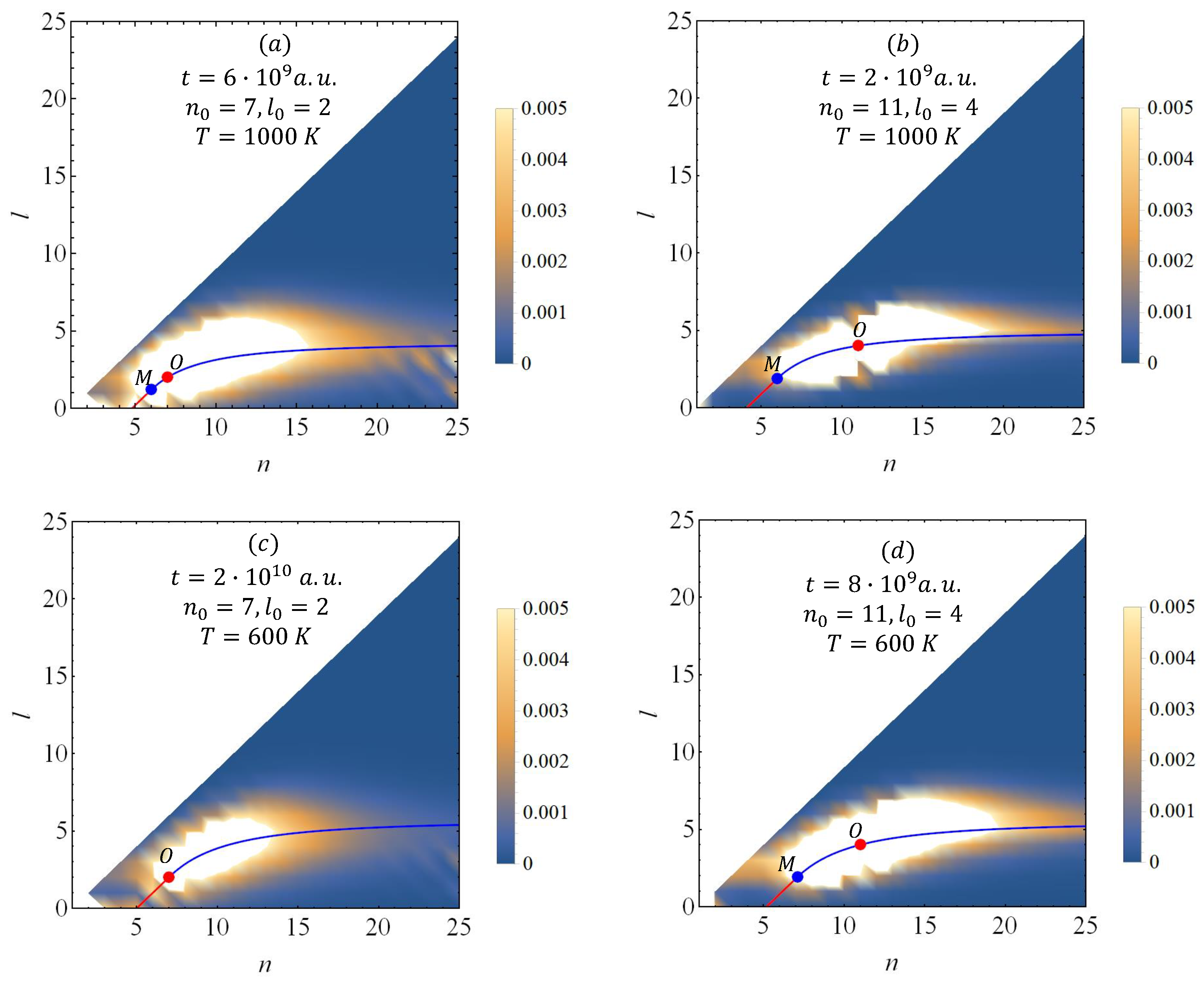
Figure 3 shows the redistribution of the population induced by blackbody radiation. The calculated main paths are also shown. The red segment of the main path is determined by (7), and the blue segment of the main path is determined by (36), where $\mathsf{\Omega }$ is defined by (41). The intersection of the segments is determined by (40). One can see that the calculated paths are in good agreement with the simulation results.

4. Conclusions

We considered diffusion-like redistribution of population between the Rydberg states in an atom due to a multistep cascade of transitions induced by a continuous-spectrum radiation. The study is based on numeric simulation of the kinetic equations and its qualitative analysis in the space of quantum numbers n, l. Explicit expressions for approximate boundaries of the redistribution region are derived as well as for the main path of the process.

Comparison of the simulation with its qualitative analysis suggests that the main features of the redistribution process are mainly independent on the intensity of competing processes such as spontaneous transitions into the ground state and the photoionization. Indeed, the simulation included both spontaneous transitions and photoionization, whereas the qualitative analysis does not include them. Nevertheless, the derived boundaries of the redistribution region and the main path presented at Figure 1 and Figure 3 are in good agreement with the simulation.

In our model, we assume the concentrations sufficiently low, therefore we do not account for collisional transitions. In addition, we do not consider the change of m due to transitions. We plan to include collisional effects and a rigorous analysis of m-mixing in our next work following the approaches used in, for example, [14,24,25,26,27,28,34]).

However, it must be noted that m-changing transitions do not significantly change main features of the redistribution process as represented in $(n,l)$-plane in the present paper. Indeed, m-changing transitions change only the absolute values of transition rates $V(nl\to n^{\prime }{l}^{\prime })$ but do not change general structure of the kinetic Equation (1) as well as the diffusion approximation which we outline here. Particularly, the boundaries of the populated area (red, green and black lines in Figure 1b) determined by the Bethe rule obviously remain the same.

The rates of the redistribution and corresponding timescales also should be the objects of further investigation.

We believe that proposed approach can be of use in analyzing laboratory experiments and astrophysical data. In particular, it probably can be useful for analysis of “Rydberg ladder”—such as multistep cascades of radiative transitions in stellar atmospheres [35,36,37,38] and nebulae, where high values of the principal quantum number $n\sim 1000$ [39] and great number of involved states make the direct simulation rather difficult.

References

- Bayfield, J.E.; Koch, P.M. Multiphoton Ionization of Highly Excited Hydrogen Atoms. Phys. Rev. Lett. 1974, 33, 258–261. [Google Scholar] [CrossRef]
- Koch, P.; van Leeuwen, K. The importance of resonances in microwave ionization of excited hydrogen atoms. Phys. Rep. 1995, 255, 289–403. [Google Scholar] [CrossRef]
- Dimitrijević, M.S.; Srećković, V.A.; Zalam, A.A.; Bezuglov, N.N.; Klyucharev, A.N. Dynamic Instability of Rydberg Atomic Complexes. Atoms 2019, 7, 22. [Google Scholar] [CrossRef] [Green Version]
- Leopold, J.G.; Percival, I.C. Ionisation of highly excited atoms by electric fields. III. Microwave ionisation and excitation. J. Phys. B At. Mol. Phys. 1979, 12, 709–721. [Google Scholar] [CrossRef]
- Casati, G.; Chirikov, B.V.; Shepelyansky, D.L.; Guarneri, I. New Photoelectric Ionization Peak in the Hydrogen Atom. Phys. Rev. Lett. 1986, 57, 823–826. [Google Scholar] [CrossRef]
- Galvez, E.J.; Sauer, B.E.; Moorman, L.; Koch, P.M.; Richards, D. Microwave Ionization of H Atoms: Breakdown of Classical Dynamics for High Frequencies. Phys. Rev. Lett. 1988, 61, 2011–2014. [Google Scholar] [CrossRef] [PubMed]
- Delone, N.B.; Kraĭnov, B.P.; Shepelyanskiĭ, D.L. Highly-excited atoms in the electromagnetic field. Sov. Phys. Uspekhi 1983, 26, 551–572. [Google Scholar] [CrossRef]
- Casati, G.; Chirikov, B.V.; Shepelyansky, D.L.; Guarneri, I. Relevance of classical chaos in quantum mechanics: The hydrogen atom in a monochromatic field. Phys. Rep. 1987, 154, 77–123. [Google Scholar] [CrossRef]
- Delone, N.; Zon, B.; Krainov, V. Diffusion mechanism of ionization of highly excited atoms in an alternating electromagnetic field. Sov. Phys. JETP 1978, 48, 223–227. [Google Scholar]
- Astapenko, V.A.; Lisitsa, V.S. Interaction of Ultrashort Laser Pulses with Atoms in Plasmas. Atoms 2018, 6, 38. [Google Scholar] [CrossRef] [Green Version]
- Gallagher, T.F.; Cooke, W.E. Interactions of Blackbody Radiation with Atoms. Phys. Rev. Lett. 1979, 42, 835–839. [Google Scholar] [CrossRef]
- Glukhov, I.L.; Nekipelov, E.A.; Ovsiannikov, V.D. Blackbody-induced decay, excitation and ionization rates for Rydberg states in hydrogen and helium atoms. J. Phys. B At. Mol. Opt. Phys. 2010, 43, 125002. [Google Scholar] [CrossRef]
- Anderson, S.E.; Younge, K.C.; Raithel, G. Trapping Rydberg Atoms in an Optical Lattice. Phys. Rev. Lett. 2011, 107, 263001. [Google Scholar] [CrossRef] [PubMed]
- Seiler, C.; Agner, J.A.; Pillet, P.; Merkt, F. Radiative and collisional processes in translationally cold samples of hydrogen Rydberg atoms studied in an electrostatic trap. J. Phys. B At. Mol. Opt. Phys. 2016, 49, 094006. [Google Scholar] [CrossRef]
- Archimi, M.; Simonelli, C.; Di Virgilio, L.; Greco, A.; Ceccanti, M.; Arimondo, E.; Ciampini, D.; Ryabtsev, I.I.; Beterov, I.I.; Morsch, O. Measurements of single-state and state-ensemble lifetimes of high-lying Rb Rydberg levels. Phys. Rev. A 2019, 100, 030501. [Google Scholar] [CrossRef] [Green Version]
- Burkhardt, C.E.; Corey, R.L.; Garver, W.P.; Leventhal, J.J.; Allegrini, M.; Moi, L. Ionization of Rydberg atoms. Phys. Rev. A 1986, 34, 80–86. [Google Scholar] [CrossRef] [PubMed]
- Kaulakis, B.P. Diffusion ionization of Rydberg atoms due to black-body radiation. Sov. Phys. JETP Lett. 1988, 47, 360–362. [Google Scholar]
- Galvez, E.J.; Lewis, J.R.; Chaudhuri, B.; Rasweiler, J.J.; Latvakoski, H.; De Zela, F.; Massoni, E.; Castillo, H. Multistep transitions between Rydberg states of Na induced by blackbody radiation. Phys. Rev. A 1995, 51, 4010–4017. [Google Scholar] [CrossRef] [PubMed]
- Ryabtsev, I.I.; Tretyakov, D.B.; Beterov, I.I. Applicability of Rydberg atoms to quantum computers. J. Phys. B At. Mol. Opt. Phys. 2005, 38, S421–S436. [Google Scholar] [CrossRef] [Green Version]
- Beterov, I.I.; Tretyakov, D.B.; Ryabtsev, I.I.; Entin, V.M.; Ekers, A.; Bezuglov, N.N. Ionization of Rydberg atoms by blackbody radiation. New J. Phys. 2009, 11, 013052. [Google Scholar] [CrossRef] [Green Version]
- Beterov, I.I.; Tretyakov, D.B.; Ryabtsev, I.I.; Ekers, A.; Bezuglov, N.N. Ionization of sodium and rubidium nS, nP, and nD Rydberg atoms by blackbody radiation. Phys. Rev. A 2007, 75, 052720. [Google Scholar] [CrossRef] [Green Version]
- Beterov, I.I.; Ryabtsev, I.I.; Tretyakov, D.B.; Entin, V.M. Quasiclassical calculations of blackbody-radiation-induced depopulation rates and effective lifetimes of Rydberg nS, nP, and nD alkali-metal atoms with n ≤ 80. Phys. Rev. A 2009, 79, 052504. [Google Scholar] [CrossRef] [Green Version]
- Lopez-Puertas, M.; Taylor, F.W. Non-LTE Radiative Transfer in the Atmosphere; Series on Atmospheric Oceanic and Planetary Physics; World Scientific: Singapore, 2001; Volume 3. [Google Scholar]
- Kaulakys, B.; Ciziunas, A. A theoretical determination of the diffusion-like ionisation time of Rydberg atoms. J. Phys. B At. Mol. Phys. 1987, 20, 1031–1038. [Google Scholar] [CrossRef]
- Bezuglov, N.N.; Borodin, V.M.; Kazanskii, A.K.; Klyucharev, A.N.; Matveev, A.A.; Orlovskii, K.V. Analysis of Fokker–Planck type stochastic equations with variable boundary conditions in an elementary process of collisional ionization. Opt. Spectrosc. 2001, 91, 19–26. [Google Scholar] [CrossRef]
- Bezuglov, N.N.; Borodin, V.M.; Eckers, A.; Klyucharev, A.N. A quasi-classical description of the stochastic dynamics of a Rydberg electron in a diatomic quasi-molecular complex. Opt. Spectrosc. 2002, 93, 661–669. [Google Scholar] [CrossRef]
- Miculis, K.; Beterov, I.I.; Bezuglov, N.N.; Ryabtsev, I.I.; Tretyakov, D.B.; Ekers, A.; Klucharev, A.N. Collisional and thermal ionization of sodium Rydberg atoms: II. Theory for nS, nP and nD states with n = 5–25. J. Phys. B At. Mol. Opt. Phys. 2005, 38, 1811–1831. [Google Scholar] [CrossRef] [Green Version]
- Geppert, P.; Althön, M.; Fichtner, D.; Ott, H. Diffusive-like redistribution in state-changing collisions between Rydberg atoms and ground state atoms. Nat. Commun. 2021, 12, 3900. [Google Scholar] [CrossRef] [PubMed]
- Chervinskaya, A.S.; Dorofeev, D.L.; Zon, B.A. Diffusion Dynamics of Rydberg States in the Field of Radiation with Continuous Spectrum. Opt. Spectrosc. 2021, 129, 911–917. [Google Scholar] [CrossRef]
- Maeda, H.; Gurian, J.H.; Gallagher, T.F. Population transfer in the Na s-p Rydberg ladder by a chirped microwave pulse. Phys. Rev. A 2011, 84, 063421. [Google Scholar] [CrossRef] [Green Version]
- Bethe, H.A.; Salpeter, E.E. Quantum Mechanics of One- and Two-Electron Atoms; Dover Publications: Mineola, NY, USA, 2014. [Google Scholar]
- Lifschitz, E.M.; Pitajewski, L.P. Physical Kinetics; Butterworth-Heinemann: Oxford, UK, 1981. [Google Scholar] [CrossRef]
- Goreslavskii, S.; Delone, N.; Krainov, V. Probabilities of radiative transitions between highly excited atomic states. Sov. Phys. JETP 1982, 55, 1032–1036. [Google Scholar]
- Dorofeev, D.L.; Zon, B.A. Mixing of Rydberg states induced by interaction with moving ion. J. Chem. Phys. 1997, 106, 9609–9617. [Google Scholar] [CrossRef]
- Chang, E.S.; Noyes, R.W. Identification of the solar emission lines near 12 microns. Astrophys. J. Lett. 1983, 275, L11–L13. [Google Scholar] [CrossRef]
- Chang, E.S. Non-penetrating Rydberg states of silicon from solar data. J. Phys. B At. Mol. Phys. 1984, 17, L11–L17. [Google Scholar] [CrossRef]
- Sundqvist, J.O.; Ryde, N.; Harper, G.M.; Kruger, A.; Richter, M.J. Mg I emission lines at 12 and 18 μm in K giants. A&A 2008, 486, 985–993. [Google Scholar] [CrossRef] [Green Version]
- Carlsson, M.; Rutten, R.; Shchukina, N. The formation of the Mg I emission features near 12 microns. Astron. Astrophys. 1992, 253, 567–585. [Google Scholar]
- Gulyaev, S.; Nefedov, S. Populations of Rydberg states of atoms in nebulae. Astron. Nachrichten 1991, 312, 27–31. [Google Scholar] [CrossRef]
Figure 1.
(Color online) The redistribution of the population in the space of quantum numbers n and l. The initial state is . The incident radiation has a rectangular spectrum with , and a spectral density ; (a) , (b) The magnitude of the population is shown in color. The boundaries (5), (7) and (9) are shown by red, green and black curves, respectively; the main path (36) is shown by a blue line. Point O corresponds to the initial state, point Q corresponds to (6), (8), and point M is the point of deflection (31) of the main path from the red line.
Figure 2.
(Color online) (a) Local diffusion ellipse. The main diffusion direction e corresponds to the main axis of this ellipse and forms an angle to the n axis. (b) The vector field e. The blue line corresponds to the streamline of this field. The initial state is shown by the red point.
Figure 3.
(Color online) The redistribution of the population within the space of quantum numbers n and l due to blackbody radiation. The magnitude of the population is shown in color, the red line is given by (7) and the blue line is given by (36) with defined by (41). Point O indicates the initial state, and point M is the point of deflection (40) of the main path from the line (7).
Publisher’s Note: MDPI stays neutral with regard to jurisdictional claims in published maps and institutional affiliations. |
© 2021 by the authors. Licensee MDPI, Basel, Switzerland. This article is an open access article distributed under the terms and conditions of the Creative Commons Attribution (CC BY) license (https://creativecommons.org/licenses/by/4.0/).
Share and Cite
MDPI and ACS Style
Chervinskaya, A.S.; Dorofeev, D.L.; Zon, B.A. Redistribution of the Rydberg State Population Induced by Continuous-Spectrum Radiation. Atoms 2021, 9, 55. https://0-doi-org.brum.beds.ac.uk/10.3390/atoms9030055
AMA Style
Chervinskaya AS, Dorofeev DL, Zon BA. Redistribution of the Rydberg State Population Induced by Continuous-Spectrum Radiation. Atoms. 2021; 9(3):55. https://0-doi-org.brum.beds.ac.uk/10.3390/atoms9030055
Chicago/Turabian StyleChervinskaya, Anastasia S., Dmitrii L. Dorofeev, and Boris A. Zon. 2021. "Redistribution of the Rydberg State Population Induced by Continuous-Spectrum Radiation" Atoms 9, no. 3: 55. https://0-doi-org.brum.beds.ac.uk/10.3390/atoms9030055
Note that from the first issue of 2016, this journal uses article numbers instead of page numbers. See further details here.