Evaluation of Fe XIV Intensity Ratio for Electron Density Diagnostics by Laboratory Measurements

Abstract

The intensity ratio of Fe XIV 264.765A/274.203A is useful to determine the electron density of solar corona, and the relationship between the electron density and the intensity ratio obtained from a model should be evaluated using laboratory plasmas to estimate the electron density more precisely. We constructed a new collisional–radiative model (CR-model) for Fe XIV (an Al-like iron ion) by considering the processes of proton-impact excitation and electron-impact ionization to the excited states of a Mg-like iron ion. The atomic data used in the CR-model were calculated using the HULLAC atomic code. The model was evaluated based on laboratory experiments using a compact electron beam ion trap, called CoBIT, and the Large Helical Device (LHD). The measured Fe XIV 264.785 Å/274.203 Å line intensity ratio with CoBIT was 1.869 ± 0.036, and it agreed well with our CR-model results. Concurrently, the measured ratio using LHD was larger than the results of our CR-model and CHIANTI. The estimated electron densities using our CR-model agreed with those from CHIANTI within a factor of 1.6–2.4 in the range of $n_e\approx {10}^{10-11}{\mathrm{cm}}^{-3}$. Further model development is needed to explain the ratio in a high-electron density region.

1. Introduction

Spectroscopy provides various information on observed plasmas, and is important for obtaining their physical properties, particularly of astrophysical plasmas. Measuring a density-sensitive line intensity ratio is a good method for diagnosing the electron density of plasmas. For example, the intensity ratios of Fe XIII line pairs, such as 203.8 Å/202.0 Å, are used to estimate the electron densities of solar plasmas [1]. The model used in Watanabe et al. [1] had been examined using laboratory plasmas, and it had been validated by Yamamoto et al. [2]. 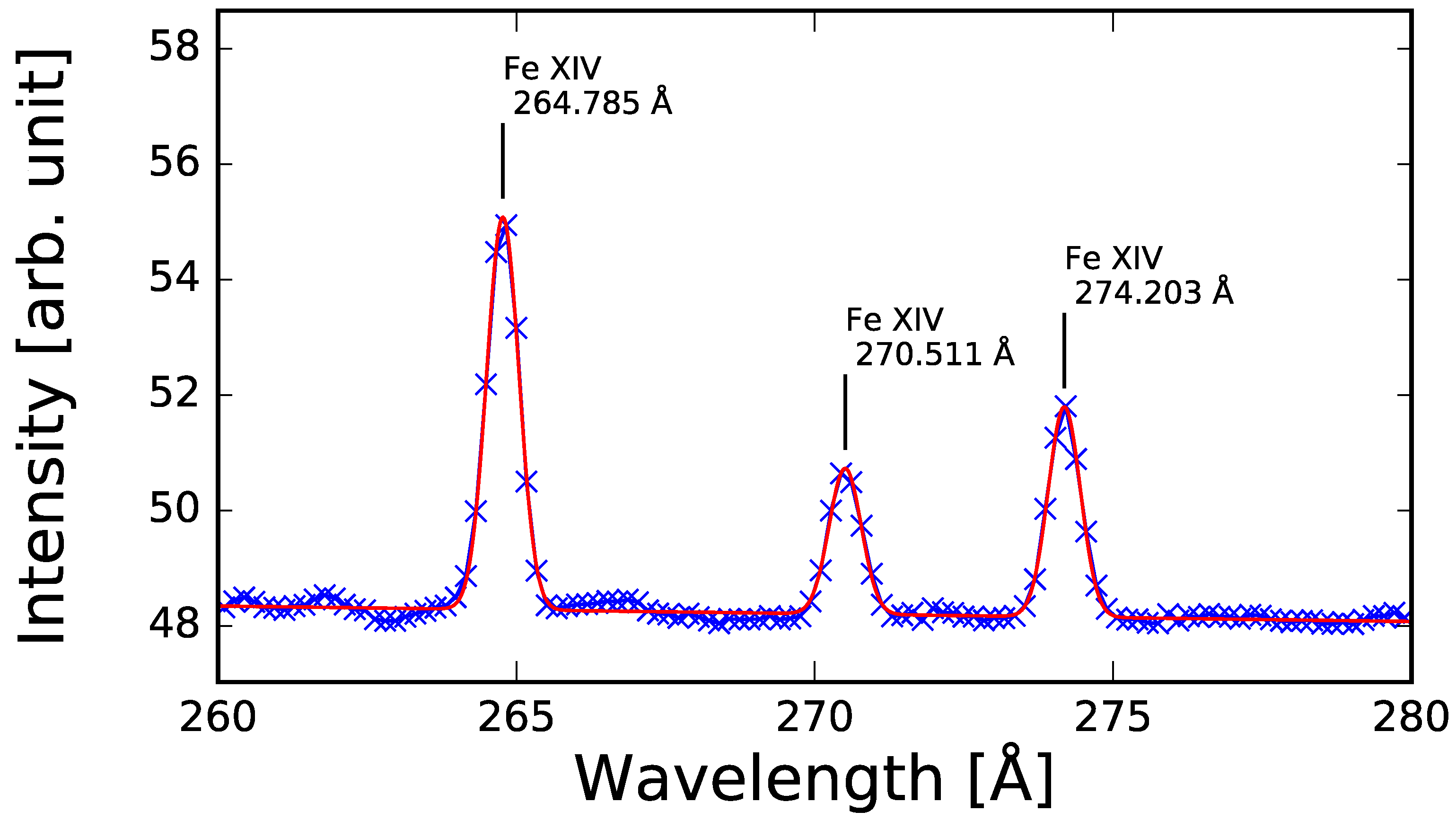The extreme ultraviolet (EUV) emission lines from the solar corona have been observed using the Solar EUV Rocket Telescope and Spectrograph (SERTS) [3] and the EUV Imaging Spectrometer (EIS) onboard the Hinode satellite [4]. The intensity ratio of Fe XIV 264.785 Å and 274.203 Å lines is sensitive to electron density, and it is one of the most measured line pairs by Hinode/EIS (e.g., References [5,6,7,8,9,10]). The ion fraction of the Al-like iron ion (Fe XIV) presents a peak in ${10}^{6.3}\mathrm{K}$ plasmas; thus, measuring the Fe XIV 264.785 Å/274.203 Å line intensity ratio is a good method for electron density diagnosis for plasma phenomena in the solar corona.

A collisional–radiative model (CR-model) is used to derive the relationship between the intensity ratio and the electron density. For reliable density diagnostics, the CR-model should be evaluated by laboratory plasma measurements. To understand the dynamics of solar plasmas, such as the chromospheric evaporation by accelerated particles (e.g., Reference [11]), a reliable CR-model is needed.

The CR-model included in CHIANTI [12] is frequently used for the analysis of solar plasmas. In CHIANTI ver. 9 [12,13], the atomic data for Fe XIV are mainly taken from Liang et al. [14]. The CR-model for Fe XIV in CHIANTI considers 739 fine-structure levels with electron configurations $\left\{3s^{x}3p^{y}3d^z\right\}(x+y+z=3)$, $3s^{2}nl(nl=4s-7i)$, $3s3pnl(nl=4s-6p)$, and $3s3d4l(l\in \{s,p,d,f\left\}\right)$. The included transitions for electron-impact excitation/de-excitation and radiation are limited. The electron-impact ionization processes from the excited levels to the ground and other excited states of the Mg-like iron ions are excluded. The proton-impact excitation process between two fine-structure levels of the ground state is included. CHIANTI is aimed mainly for application to low-density solar plasmas; therefore, the collision processes between excited levels are not significantly important and subsequently omitted.

From the aspect of model evaluation, laboratory experiments using electron beam ion traps (EBITs) are reported for the Fe XIV 264.785 Å/274.203 Å intensity ratio, and the measured results are roughly consistent with those obtained with CHIANTI within $n_e\approx {10}^{10-11}{\mathrm{cm}}^{-3}$ [15,16]. In a high-electron density region, magnetically confined plasmas can be used to evaluate a model. Plasma experiments with the NSTX-U tokamak measured the Fe XIV 274.203 Å/264.785 Å line intensity ratio [17]. Weller et al. [17] did not consider the Fe XIV 264.785 Å line blending with a Fe XV 265.00 Å, although an Fe XVI 262.98 Å line was observed in their spectra. The above-mentioned line blending could not be resolved in their experiments. The obtained Fe XIV 264.785 Å/274.203 Å line intensity ratio was approximately 3–4, which is much larger than the intensity ratio calculated using CHIANTI ver. 9. On setting the weak emission line (274.203 Å) intensity as the numerator, the intensity ratios were small values, as shown in the figures in their study, and were much smaller than the calculation by CHIANTI. However, they did not discuss this difference between their measured values and the calculations by CHIANTI, and concluded that the experimental results agreed with the calculations.

In this study, we focus on the difference between experimental and model calculation results, and construct a new CR-model using the atomic data calculated with the HULLAC atomic code [18]. Electron-impact excitation and ionization cross-sections are obtained using a distorted-wave method, which yields reasonably good cross-sections for a wide collision energy range. In our CR-model, we include the electron-impact excitation and de-excitation processes between all ground and excited states of an Al-like iron ion, electron-impact ionization processes from the excited levels of an Al-like iron ion to the ground and excited states of a Mg-like iron ion, and proton-impact excitation and de-excitation processes between the fine-structure levels of the ground state. We investigate their effects on the intensity ratio. The details of the CR-model are described in Section 2. The CR-model is evaluated against laboratory experiments conducted using a compact electron beam ion trap (CoBIT) and the Large Helical Device (LHD) at the National Institute for Fusion Science (NIFS), and the examination of the measured spectra is presented in Section 3. We discuss the model validity against the experimental results in Section 4 and present conclusions in Section 5.

2. Collisional–Radiative Model

In this section, we describe the details of the newly developed CR-model in this study. The CR-model provides the population densities of excited states relative to that of the ground state under a quasi-steady state assumption. It solves the rate equations of the change in the population densities of the excited states. When the timescales of the atomic processes changing the population densities of the excited states are sufficiently shorter than that of the changing plasma conditions, the steady-state assumption is valid. Consequently, we can easily determine the population densities by solving the inverse matrix of the rate coefficients in the rate equations. We construct the CR-model as follows: (1) first, the atomic structure and cross-sections are calculated; (2) subsequently, the rate coefficients are calculated by averaging the cross-sections with the Maxwellian velocity distribution function; and, (3) finally, the rate equation is solved.

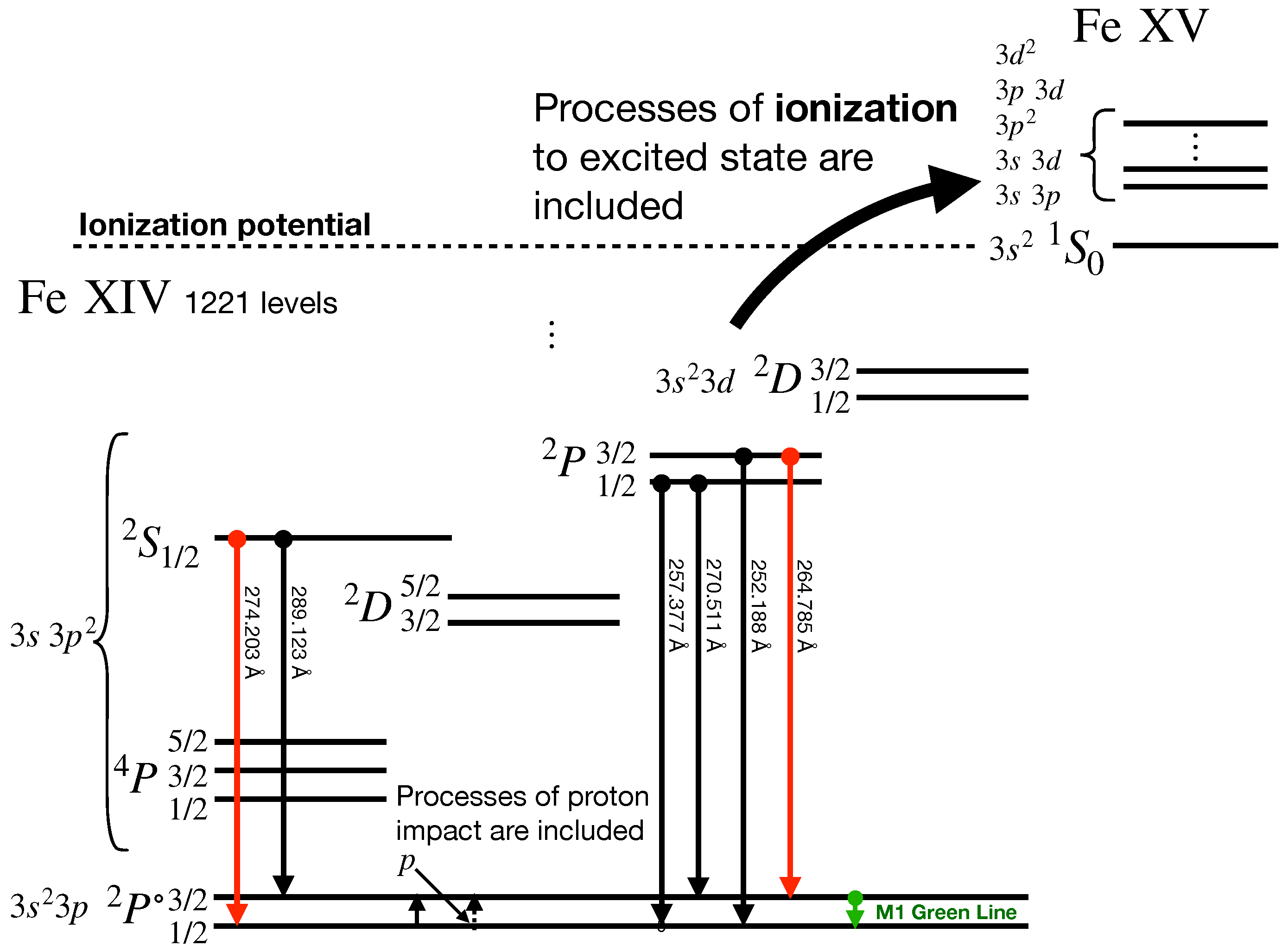
The atomic structure is calculated with the lowest 1221 fine-structure levels of $3s^{x}3p^{y}3d^z$ $\left(x+y+z=3\right)$, $3s^{2}nl$, $3s3pnl$, $3s3dnl$, $3p^{2}nl$, $3p3d4l$ ($n=4\mathrm{or}5;$ $l=s,p,d\mathrm{or}f$), and $3d^{2}4l(l=s,p\mathrm{or}d)$. A radiative decay between the fine-structure levels of the ground state, $3s^{2}3p{}^2{P}_{3/2}^{\circ }-{}^2{P}_{1/2}^{\circ }$ (see Figure 1), was presented by Edlen [19] as the forbidden M1 line, which is known as the “green line” (e.g., Reference [20]). This forbidden transition makes $3s^{2}3p{}^2{P}_{3/2}^{\circ }$ a metastable state. The electron density dependence of the Fe XIV electron density-dependent line ratios was considered to be due to this metastable state.

In this study, we consider electron-impact excitation, de-excitation and ionization, radiative decay, and proton-impact excitation and de-excitation processes. We consider the electron-impact ionization processes from the ground and excited states of an Al-like iron ion to the excited states of $3s3p$, $3s3d$, $3p^2$, $3p3d$, and $3d^2$, as well as to the $3s^2$ ground state of a Mg-like iron ion. These ionization processes are not included in CHIANTI and the model in Liang et al. [14].

The rate equation for the population density of level i is written as

$$\begin{array}{cc}\hfill \frac{\mathrm{d}{n}_z\left(i\right)}{\mathrm{d}t}=& \sum _{j>i}\left\{C_e\left(j,i\right)n_e+C_p\left(j,i\right)n_p+A_r\left(j,i\right)\right\}{n}_z\left(j\right)\hfill \\ \hfill & +\sum _{k<i}\left\{F_e\left(i,k\right)n_e+F_p\left(i,k\right)n_p\right\}{n}_z\left(k\right)\hfill \\ \hfill & -\left\{\sum _{k<i}\left(C_e\left(i,k\right)n_e+C_p\left(i,k\right)n_p+A_r\left(i,k\right)\right)\right.\hfill \\ \hfill & \left.+\sum _{j>i}\left(F_e\left(j,i\right)n_e+F_p\left(j,i\right)n_p\right)+\sum _q{S}_z\left(i,q\right)\right\}{n}_z\left(i\right),\hfill \end{array}$$

(1)

where $C_e\left(j,i\right)$ and $F_e\left(j,i\right)$ are the electron-impact excitation and de-excitation rate coefficients from level j to level i, respectively; $C_p\left(j,i\right)$ and $F_p\left(j,i\right)$ are the proton-impact excitation and de-excitation rate coefficients from level j to level i, respectively; $A_r\left(j,i\right)$ is the radiative decay rate from level j to level i; and $S_z\left(i,q\right)$ is the electron-impact ionization rate coefficient from level i in the z th charged ion to level q in the $\left(z+1\right)$th charged ion. Here, z is 13.

We calculate the energy levels, transition probabilities, and the electron-impact excitation and ionization cross-sections using the HULLAC atomic code [18]. The electron-impact excitation and ionization cross-sections are calculated using a relativistic distorted-wave method. The electron-impact excitation and ionization rate coefficients are obtained by the convolution of the cross-section and electron velocity distribution function. We used Landman’s proton-impact excitation rate coefficient [21], which is recommended by Skobelev et al. [22]. According to Skobelev et al., $3s^{2}3p{}^2{P}_{1/2}^{\circ }-{}^2{P}_{3/2}^{\circ }$ is the only important transition for Fe XIV. Thus, we include only this transition in our CR-model. We calculate the de-excitation rate coefficients from the excitation rate coefficients in a detailed balance using the Klein–Rosseland relation (eq. 3.31 in Fujimoto [23]). Here, we assume that the proton density is equal to the electron density and the proton temperature is equal to the electron temperature.

To examine the effects of the proton-impact excitation and the electron-impact ionization to the excited states of a Mg-like iron ion for the line intensity ratio of Fe XIV 264.785 Å and 274.203 Å, we consider four models: (1) IoEx0p0: a model that includes neither the proton-impact excitation nor the ionization to the excited states; (2) IoEx0p1: a model that does not include the ionization to the excited states but includes the proton-impact excitation; (3) IoEx1p0: a model that does not include the proton-impact excitation but includes the ionization to the excited states; and (4) IoEx1p1: a model that includes both the proton-impact excitation and the ionization to the excited states. The electron-impact ionization to the ground state of a Mg-like iron ion is included in all models.

The line intensities of Fe XIV 264.785 Å and 274.203 Å are determined by multiplying the upper-level populations by the transition probabilities. These upper levels are $3s3p^2{}^2{P}_{3/2}$ and $3s3p^2{}^2{S}_{1/2}$, respectively, as shown in Figure 1. For level $3s3p^2{}^2{S}_{1/2}$, the population inflow from level $3s^{2}3p{}^2{P}_{3/2}^{\circ }$ by electron-impact excitation is much smaller than that from level $3s^{2}3p{}^2{P}_{1/2}^{\circ }$ by electron-impact excitation. However, for level $3s3p^2{}^2{P}_{3/2}$, the population inflow from level $3s^{2}3p{}^2{P}_{3/2}^{\circ }$ is non-negligible. Thus, the population density of level $3s3p^2{}^2{P}_{3/2}$ is affected by the population of level $3s^{2}3p{}^2{P}_{3/2}^{\circ }$, i.e., the metastable state, which is largely affected by the proton-impact excitation processes. Therefore, the proton-impact excitation contributes to the density dependence of the Fe XIV 264.785 Å/274.203 Å intensity ratio. In our calculations, the IoEx0p1 and IoEx1p1 models, which include the proton-impact excitation processes, achieve a higher Fe XIV 264.785 Å/274.203 Å intensity ratio up to 6% at electron density ${10}^{10}{\mathrm{cm}}^{-3}$ compared to the IoEx0p0 and IoEx1p0 models, respectively (see Figure 2).

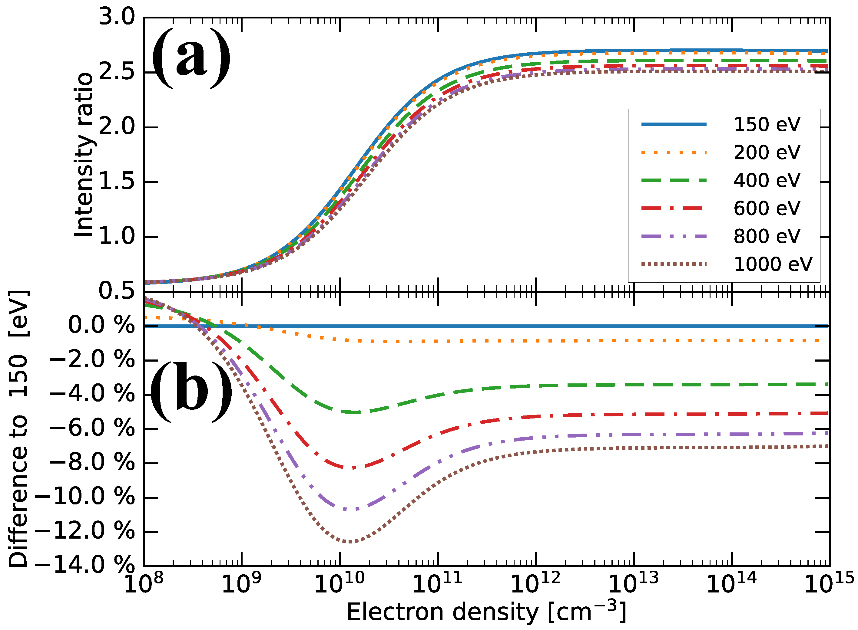
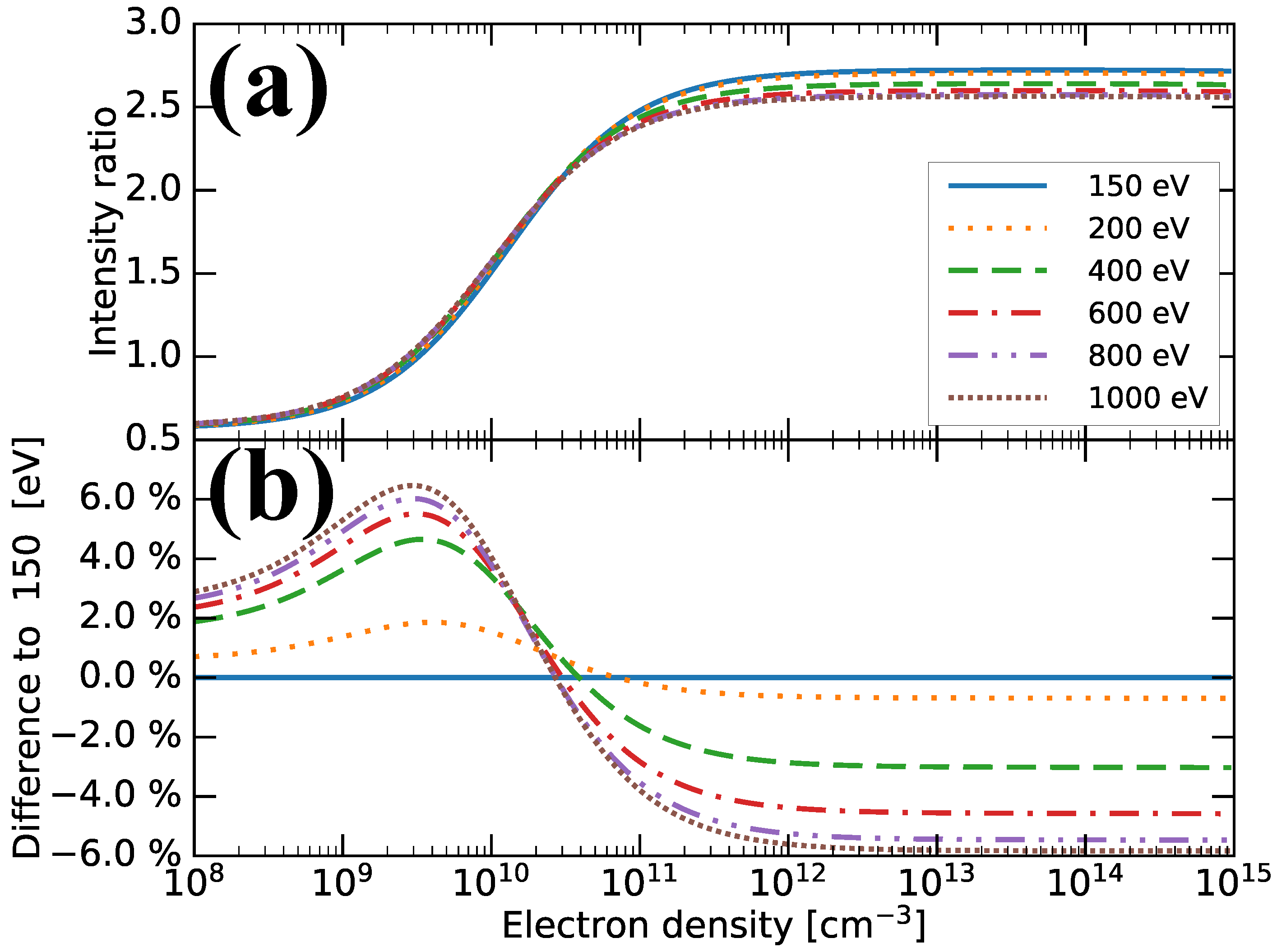
We also examine the electron-temperature dependence of the intensity ratios obtained using the four models. Figure 3 shows the electron density dependence change with electron temperature for the IoEx0p0 model. The differences in the intensity ratios relative to the 150 eV case are plotted in Figure 3b, and the maximum difference is found at an electron density of approximately ${10}^{10}{\mathrm{cm}}^{-3}$. This difference is approximately 12% between $T_e=150\mathrm{eV}$ and $T_e=1000\mathrm{eV}$. 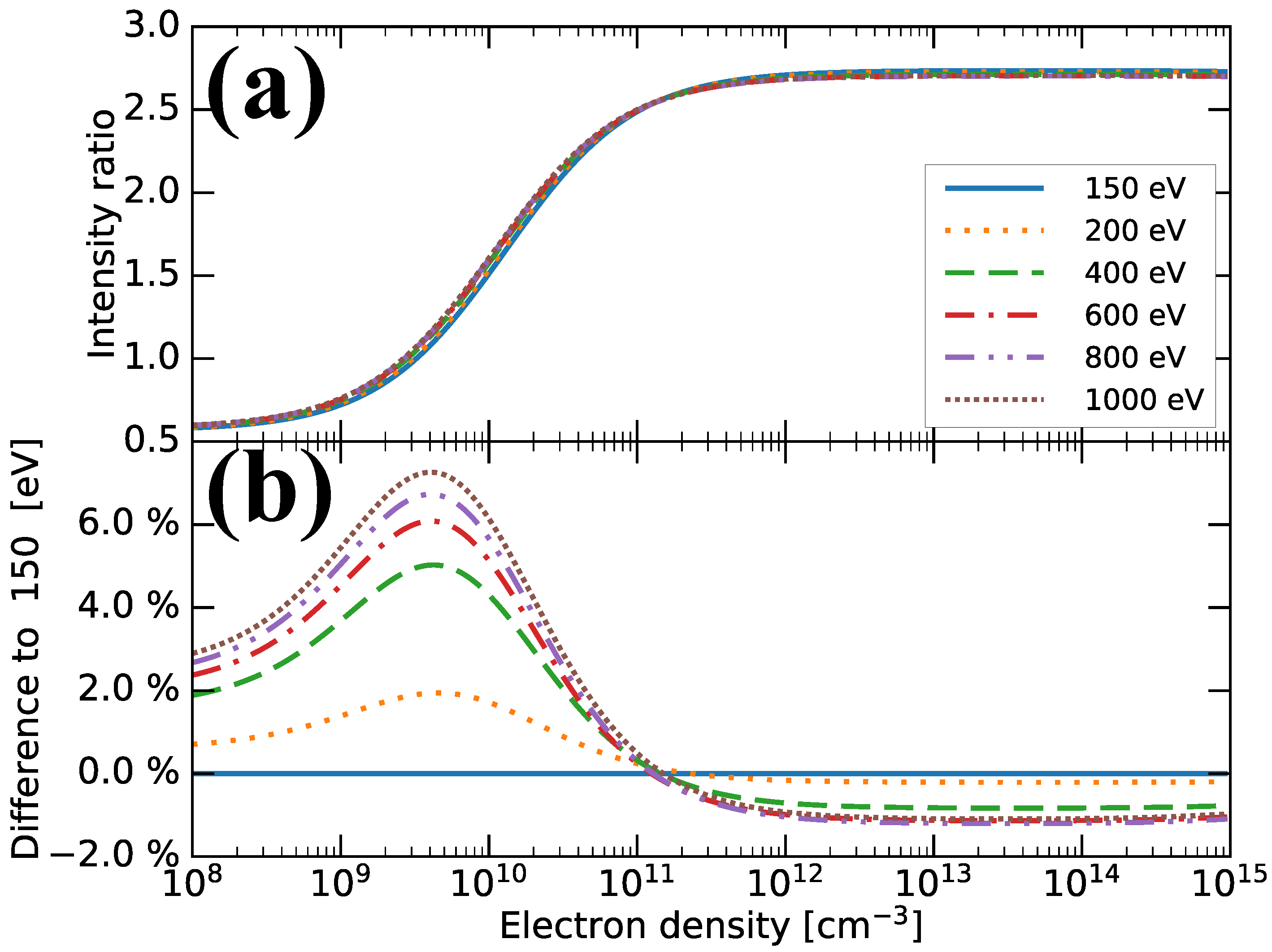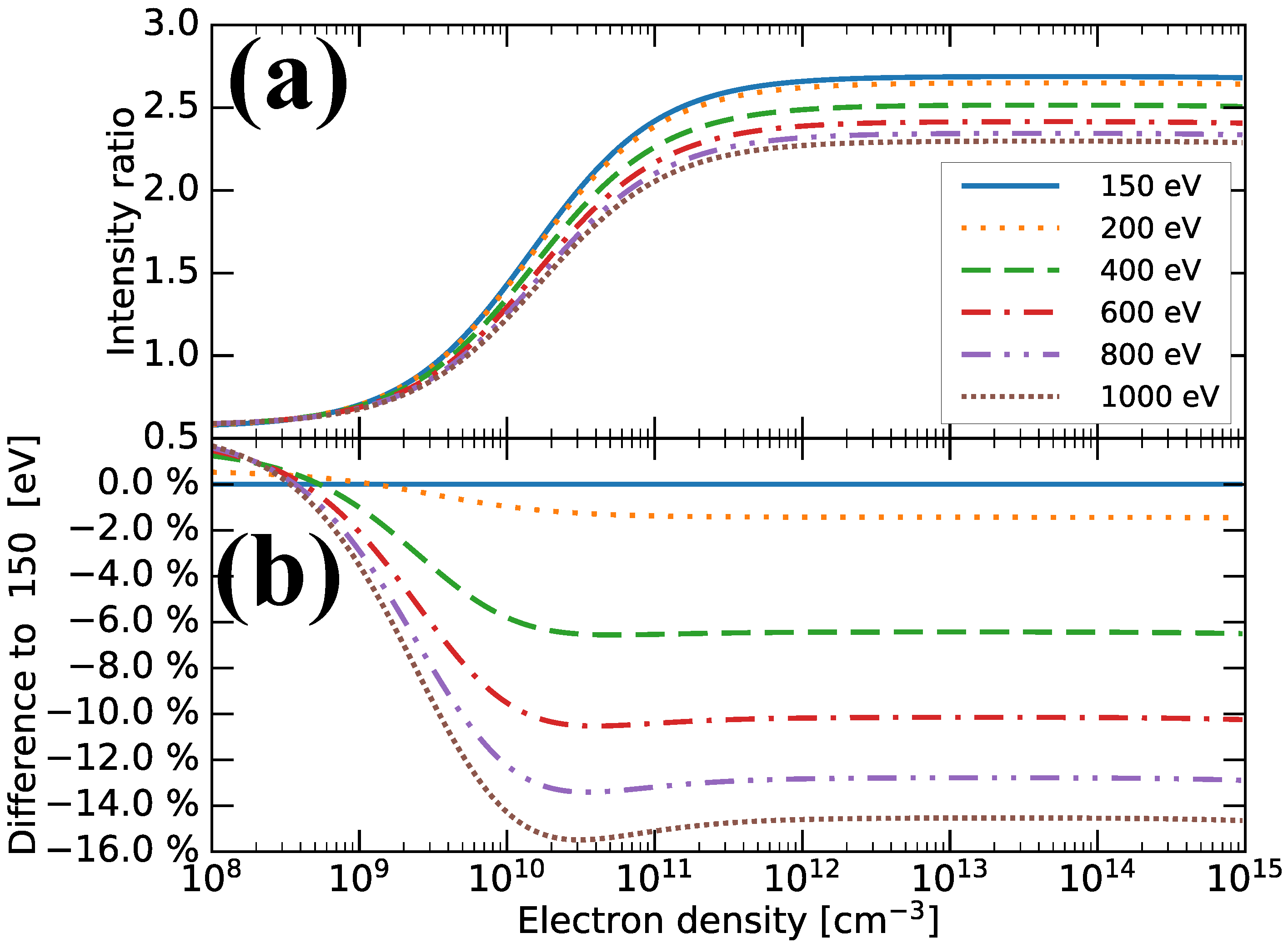When we include the proton-impact excitation effect (the IoEx0p1 model; see Figure 4), the above differences become small. The proton-impact excitation process cancels out the temperature dependence of the electron-impact excitation effects for the Fe XIV 264.785 Å/274.203 Å line intensity ratio. However, when we include the ionization processes to the excited states of Fe XV (the IoEx1p0 model; see Figure 5), the temperature dependence in the high-density region becomes larger, and the difference between $T_e=150\mathrm{eV}$ and $T_e=1000\mathrm{eV}$ becomes approximately 15%. The temperature dependence using the model that includes both the proton-impact excitation and ionization process to the excited states in Fe XV (the IoEx1p1 model) is shown in Figure 6. It suggests that the maximum difference in the intensity ratios is 6% between the 150 eV and 1000 eV cases. The proton-impact excitation processes reduce the difference. Under a high-electron temperature condition, such as 1000 eV, at which a plasma is not in ionization equilibrium, the contributions of the proton-impact excitation and ionization processes to the excited states are approximately +7% and −7%, respectively (compared to the differences in Figure 3 and Figure 4 and the differences in Figure 3 and Figure 5). Both contributions cancel each other, and the model differences in the high-density region become small (note the small difference between Figure 3 and Figure 6 in the high-density region). Summarizing the temperature dependence with the models, we find that the difference varies from −15% to 6%, and is ±6% for our best model, the IoEx1p1 model.

3. Experiments and Results

To evaluate the CR-model, we performed laboratory experiments using CoBIT [24,25] and LHD [26] at the NIFS.

3.1. CoBIT

CoBIT is an instrument that produces and traps highly charged ions in an electron beam. In the present experiment, CoBIT at the NIFS (CoBIT-II) [25] was used. Iron ions were produced by introducing $\mathrm{Fe}{\left({\mathrm{C}}_5{\mathrm{H}}_5\right)}_2$ vapor into CoBIT-II. The EUV spectrometer mounted on CoBIT-II was composed of a 1200 gr/mm grating (30-002 Shimadzu Corporation) and a charge coupled device. Because the spectrometer was used in the slit-less configuration, the wavelength resolution was mainly limited by the line source width (typically several hundred micrometers). To avoid line blending of Fe XIV 264.785 Å and Fe XVI 265.000 Å, the beam energy was set as 400 eV, which is less than 456.2 eV, the ionization energy of Fe XV. The electric current was set as 10.0 mA. Although the profile of the electron beam was not measured directly, we refer the electron density measured with CoBIT at the University of Electro-Communications (CoBIT-I) [15] with the same electron current. This is because we assume same systems with the same electric currents, same magnetic fields, and same beam energies produce the same electron beam radius and the same electron density.

We recorded the spectrum (Figure 7) for a 3600 s integration, and the lines were fitted with a Gaussian profile to estimate the intensities. The Fe XIV 264.785 Å/274.203 Å intensity ratio was obtained as 1.869 ± 0.036 after line profile fitting. The intensity ratios measured with CoBIT-II (this study) and CoBIT-I [15] were consistent (Figure 8). Note that we assumed the sensitivities of the lines to not be significantly different because of the closeness of the measured lines. We discuss the details of the model evaluation in Section 4.

3.2. Large Helical Device

3.2.1. Experimental Setup and Overview of Experiments

LHD is a fusion research device that can confine plasma magnetically. We performed experiments on 6 December 2019. LHD plasmas were heated by electron cyclotron resonance heating at the beginning, and the plasmas were kept by neutral beam injection (NBI) heating. To measure the Fe XIV lines, we injected an iron pellet [27] into the plasma at approximately 4.5 s. We used a flat-field EUV spectrometer [28] and converted the measured count rates to photon flux using the relation described in Chowdhuri et al. [28].

Fe XIV lines were observed in the discharges of shot numbers 156587, 156589–156593, 156598, 156599, and 156601–156606. We successfully measured Fe XIV lines immediately before the plasma collapsed or when a hollow distribution of electron temperatures with a very low temperature at the plasma center was produced.

One example of the former cases is shown in Figure 9. The spectrum at t = 4.64 s is shown in Figure 9a, and the spatial distributions of the electron temperature and density from the Thomson scattering mapping (TSMAP) database [29] are shown in Figure 9b. Smoothly fitted profiles of the electron temperatures and densities were obtained from Thomson scattering measurements. At the time when Fe XIV lines were measured, the electron temperature at the center was extremely high for Al-like iron ions to exist. This suggests the emission of Fe XIV may originate from the edge region of the plasmas.

The time evolution of the plasma properties showed that the radiation power (red solid line in Figure 9d) increased after the iron pellet injection at 4.56 s. Simultaneously, the electron temperature (red dot-dot-dashed line in Figure 9e) at the center (normalized minor radius $\rho =0$) began to decrease owing to the radiation power loss, and the electron density at the center increased (blue dashed line in Figure 9e). The power of NBI heating (green dashed line in Figure 9d) became the half accidentally at 4.6 s, and the plasma started to collapse, as indicated by the rapid increase in the radiation power.

In the discharge of shot number 156606, the time evolution of the plasma was different, as shown in Figure 10. After the NBI heating was switched from tangential NBI to radial NBI, the central electron temperature decreased (Figure 10e), and a hollow electron temperature distribution was produced by the strong radiation power due to the iron accumulation at the center, as shown in Figure 10b. The plasma was maintained stably with a low central electron temperature for some time. Fe XIV lines were measured at t = 6.405 s (Figure 10a) when the electron temperature and density distributions were hollow shaped. Therefore, the Fe XIV emission possibly originated from the central region of the plasma.

3.2.2. Spectra Analysis

We derived the line intensities by fitting the spectra with Gaussian profiles. In the spectra, Fe XIV 264.780 Å and Fe XVI 265.000 Å were blended; therefore, we estimated the intensity of Fe XVI 265.003 Å from the intensity Fe XVI 262.976 Å by CHIANTI ver. 9 [12,13] calculations to extract the contribution of Fe XVI 265.000 Å from the intensity of Fe XIV 264.785 Å. The line centers of Fe XIV 264.785 Å and Fe XVI 265.000 Å were fixed by the wavelengths listed in the NIST Atomic Spectral Database [30] relative to the fitted Fe XVI 262.976 Å, Fe XIV 270.511 Å, and Fe XIV 274.203 Å central wavelengths.

To exclude noise and other lines during the fitting procedure, we adopted the concept of Chauvenent’s criterion (cf. Reference [31]), i.e., rejecting a datum if the product of probability of that datum point and the number of data points is less than 0.5. The excluded data points are shown as red crosses, instead of blue dots, in Figure 9a and Figure 10a.

3.2.3. Estimation of Electron Density around Al-like Iron Ion

The flat-field EUV spectrometer on LHD does not have spatial resolution, and the spectra were measured as integrated signals along the line of sight. Thus, there was no information about the spatial distribution on the abundance of Al-like iron ions. Al-like iron ions are expected to exist in a certain electron temperature region. When we estimate the electron density of the plasma where Fe XIV lines are emitted, we should exclude the region where the electron temperature is extremely high or extremely low for Al-like iron ions to exist. Therefore, we calculated the ion abundance distribution in ionization equilibrium using CHIANTI ver. 9 [12,13] using the fitted electron temperature distribution from TSMAP (Figure 9c and Figure 10c). In CHIANTI, ion abundances in ionization equilibrium are calculated under coronal approximation [32], and no density effects are included. Using CHIANTI, the most abundant electron temperature for Al-like iron ions in ionization equilibrium is obtained as 168 eV. Electron densities of LHD plasmas of approximately ${10}^{13}{\mathrm{cm}}^{-3}$ generally require including the density effect in ionization equilibrium calculations as ADAS calculations show [33]. ADAS yields the most abundant temperatures for ${10}^0{\mathrm{cm}}^{-3}$ as a low-density limit case and ${10}^{13}{\mathrm{cm}}^{-3}$ electron densities as approximately 160 eV and 140 eV, respectively. This difference is not highly significant for our purpose. Therefore, the average electron density weighted by the ion fraction calculated with CHIANTI was adopted as the electron density around Al-like iron ions.

We take root mean squares of the errors from the measurements and spatial distribution of the Al-like iron ions. The average error weighted by the ion fraction was adopted as the error from the measurements. We derive the error from the spatial distribution as follows: (1) the squared residuals are sorted; (2) the sum of the relative weights is taken; and (3) the squared residual at the point when the sum of the relative weight equals 68% is taken as the squared error.

The measured intensity ratios are plotted against the electron density in Figure 11. Our measurements using LHD are consistent with the measurements on NSTX-U [17]. The details on the evaluation of the model are discussed in Section 4.

4. Discussion

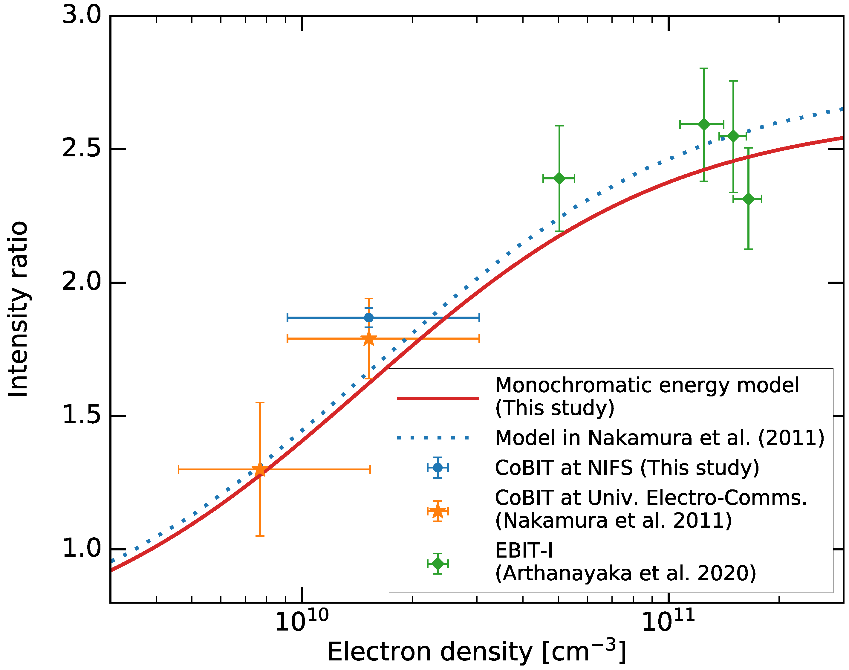
The Fe XIV 264.785 Å/274.203 Å line intensity ratios obtained from the measurements in the EBIT experiments are compared with the value calculated using the CR-model assuming a monochromatic electron energy distribution, as shown in Figure 8. The line intensity ratios obtained from the measurements in thermal plasmas are compared with the calculation result using the CR-model assuming a Maxwellian electron velocity distribution function in Figure 11.

For the CR-model with monochromatic electron energy, we use the same atomic data as in the Maxwellian velocity distribution case, except that the rate coefficients of the electron-impact excitation and ionization processes are obtained as products of the cross-sections and the collision velocities. The intensity ratios measured using CoBIT-II at the NIFS (this study), CoBIT-I at the University Electro-Communications [15], and EBIT-I at Lawrence Livermore National Laboratory [16] are consistent with our model (solid line in Figure 8). For comparison, the model calculation in [15] is shown as a dotted line in Figure 8, and it is also consistent with the measured ratios.

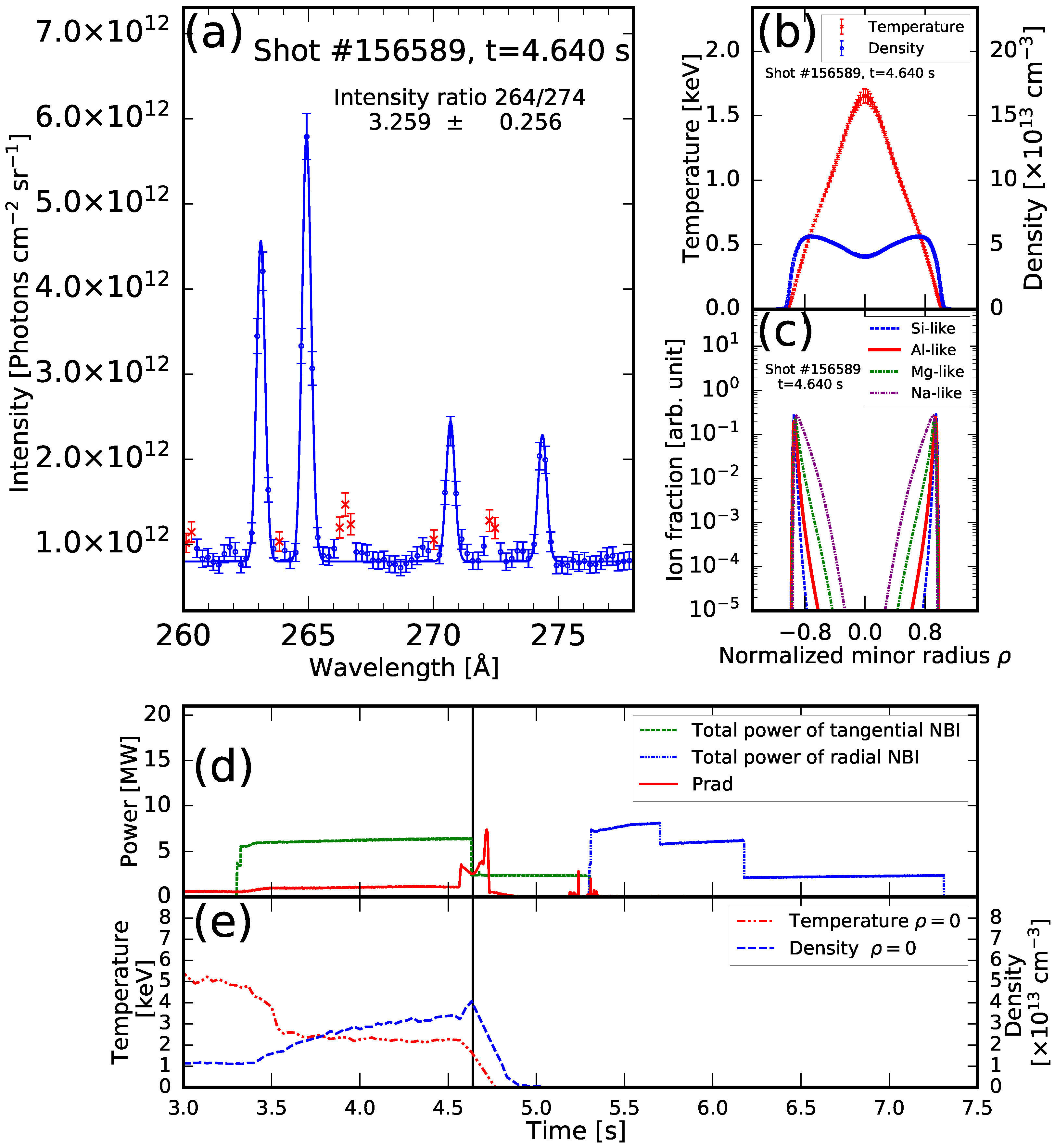
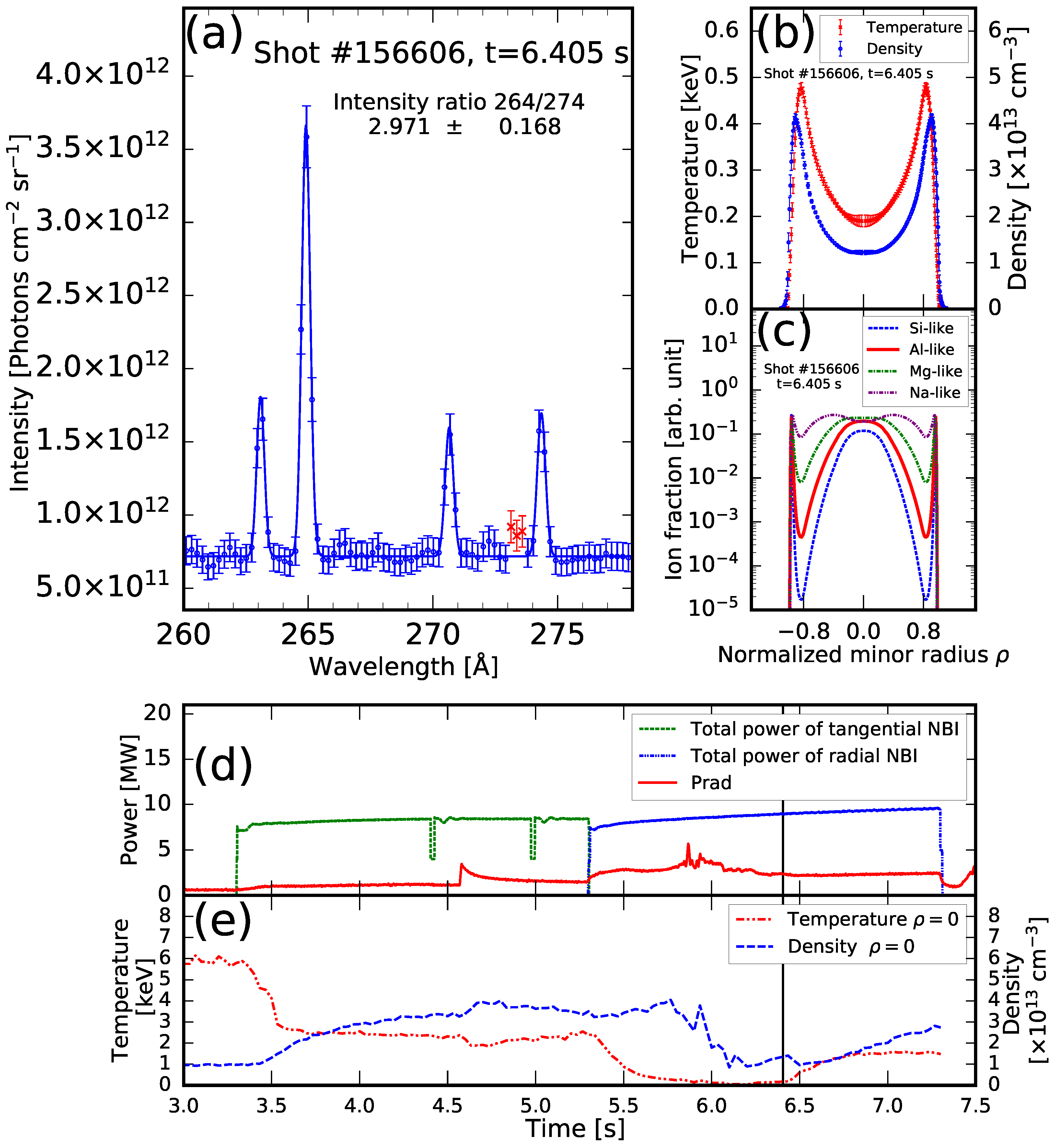
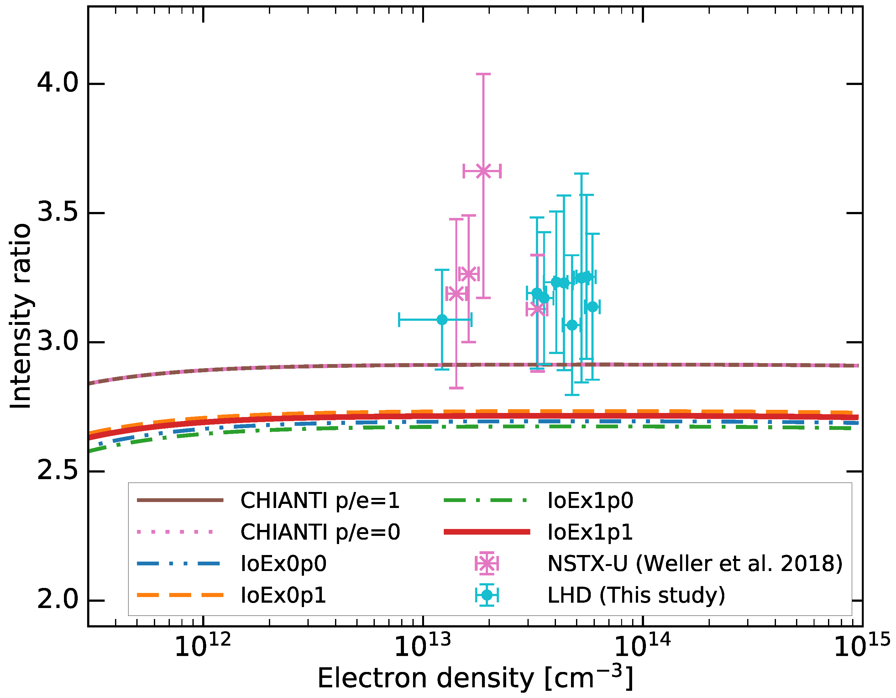
The intensity ratios measured in magnetically confined plasmas are in range of the high electron density limit. Our measurements using LHD are consistent with those with NSTX-U [17], as shown in Figure 11. However, these experimental results (NSTX-U and LHD) are larger than the model calculations. The model calculations are obtained with temperature $T_e=T_p=168\mathrm{eV}$, at which the Al-like iron ion is the most abundant according to the CHIANTI ionization equilibrium calculations, as described in Section 3.2.2.

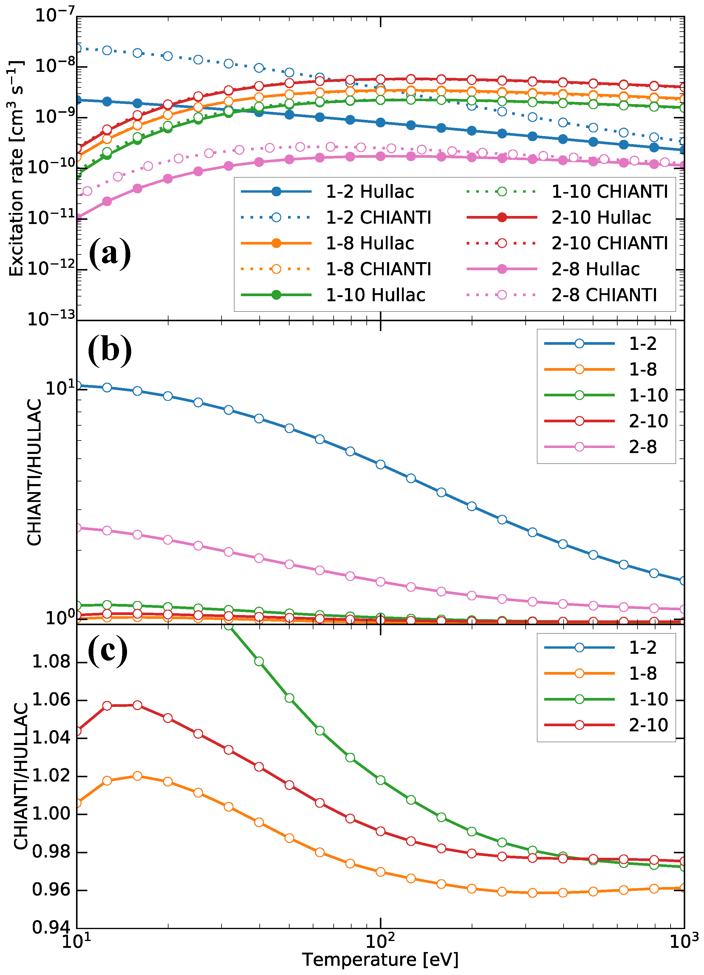
One of the largest differences between CHIANTI and our model is in the electron-impact excitation cross-sections, i.e., CHIANTI uses the cross-sections calculated with an R-matrix method, whereas we use those calculated with the distorted wave method in HULLAC. The R-matrix method can consider resonant excitation processes. We compare the differences in the electron excitation rate coefficients for several transitions, as shown in Figure 12. The excitation rate coefficients for the $3s^{2}3p{}^2{P}_{1/2}^{\circ }$ − ${}^2{P}_{3/2}^{\circ }$ (1–2) and $3s^{2}3p{}^2{P}_{3/2}^{\circ }$ − $3s3p^2{}^2{S}_{1/2}$ (2–8) transitions are significantly enhanced by the resonant processes in the low-temperature region. The electron excitation rate coefficient for the $3s^{2}3p{}^2{P}_{1/2}^{\circ }-3s3p^2{}^2{S}_{1/2}$ (1–8) transition using CHIANTI is 3% less than that obtained with our model. The electron excitation rate coefficient for the $3s^{2}3p{}^2{P}_{3/2}^{\circ }-3s3p^2{}^2{P}_{3/2}$ (2–10) transition using CHIANTI is 1% less than that determined with our model. The difference in the intensity ratios obtained with CHIANTI and our model at $T_e=168$eV and $n_e={10}^{13}{\mathrm{cm}}^{-3}$ is approximately 7%. There are several factors that cause this difference. One is the radiative transition rate, and its difference is approximately 2%. To examine the effect of enhanced excitation rate coefficients by resonance, we substituted those of the 1–2 transition from CHIANTI into our model, and we found that it leads to a 2% difference in the intensity ratio. 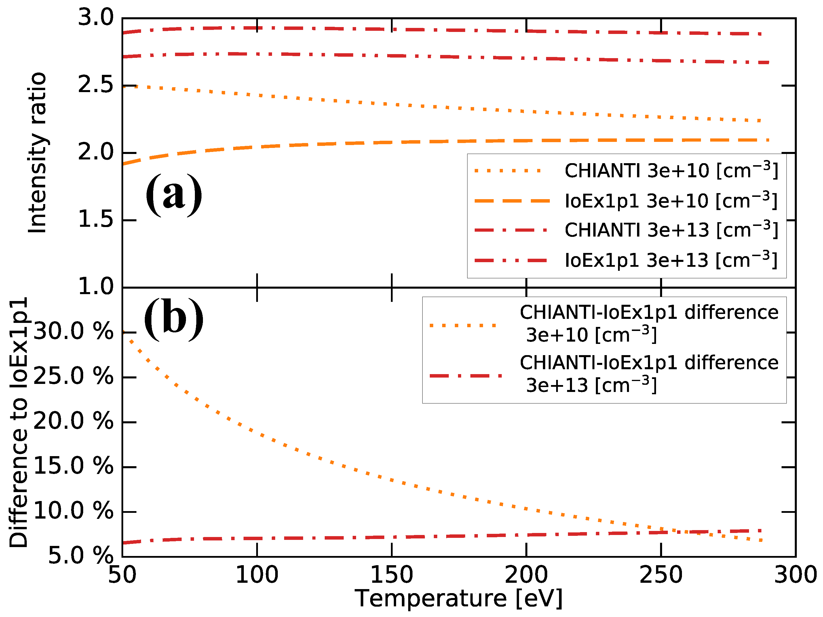Note that the CHIANTI model does not include the electron-impact ionization processes from the excited states to the ground and excited states of a Mg-like iron ion, and these processes lower the intensity ratio by approximately 1% (see Figure 2). The difference in the intensity ratio also depends on the electron temperature, and it increases with decreasing electron temperature for electron density $3\times {10}^{10}{\mathrm{cm}}^{-3}$, as shown in Figure 13. This is due to increasing resonance effect on the electron-impact excitation rate coefficients, which are included in the R-matrix method. For electron density of $3\times {10}^{13}{\mathrm{cm}}^{-3}$, the electron temperature dependence of the difference is quite small. Further model development would be necessary to explain the difference and the experimental results.

We also examine how the estimated electron density changes with the different models in the electron density range of $n_e\approx {10}^{10-11}{\mathrm{cm}}^{-3}$. For measured line intensity ratio of 1.50, the CHIANTI ver. 9 model yields electron density ${10}^{9.80}{\mathrm{cm}}^{-3}$, whereas our CR-model yields ${10}^{9.98}{\mathrm{cm}}^{-3}$. Our electron density result is 1.56 times larger than the CHIANTI value. Our model results show acceptable consistency with the experimental data, demonstrating that the derived density around this range is reasonably reliable. Taking the line intensity ratio as 2.5, the CHIANTI ver. 9 model yields an electron density of ${10}^{10.66}{\mathrm{cm}}^{-3}$, whereas our CR-model result is ${10}^{11.05}{\mathrm{cm}}^{-3}$. Our electron density result is 2.39 times larger than the CHIANTI value.

To investigate the discrepancy between the model and experimental results in a high-electron density region, we suggest the following processes to be considered in future studies. One is the effect of high-energy proton collisions. In the LHD experiments, we heated the plasma by NBI heating. NBIs produce high-energy protons by a charge exchange process between the high-energy neutral hydrogen in the NBIs and bulk hydrogen ions. Based on Ref. [22], proton-impact excitation rate coefficients are large in a high-temperature region. We assumed that protons and electrons have the same temperatures, as mentioned in Section 2. If there are many high-energy protons, this process may enhance the population density of the upper level of the 264 Å line and, hence, may increase the intensity ratio, as speculated from the comparison of Figure 5 and Figure 6. The other process is the electron-impact ionization from a Si-like iron ion. The direct ionization from excited state $3s3p^3$ of a Si-like iron ion to excited state $3s3p^2$ of an Al-like iron ion and the inner-shell ionization from the ground state $3s^{2}3p^2$ of a Si-like iron ion to excited state $3s3p^2$ might enhance the population densities of the $3s3p^2$ levels. This process could change the intensity ratio.

5. Conclusions

We constructed the new CR-model for Fe XIV, and the proton-impact excitation [22] and electron-impact ionization process from excited states to excited states $3s^{}3p$, $3s^{}3d$, $3p^2$, $3p^{}3d$, and $3d^2$, as well as ground state $3s^2$ of a Mg-like iron ion, are included. The electron density dependence of the Fe XIV 264.785 Å/274.203 Å intensity ratio is obtained for a wide density range, and the electron temperature dependence and the effects of the proton-impact excitation and electron-impact ionization to the excited states are examined. Our model results of electron density for mono-energy agree well with the experimental results obtained with EBITs, while the estimated electron density for the Maxwellian electron velocity distribution is 1.6–2.4 times larger than that using CHIANTI ver. 9 in the electron density range of $n_e\approx {10}^{10-11}{\mathrm{cm}}^{-3}$. In a comparatively higher density region ($n_e>{10}^{13}{\mathrm{cm}}^{-3}$), the LHD and NSTX-U [17] experimental results are consistent; however, the calculated ratios with both our CR-model and CHIANTI are smaller than them. The proton-impact excitation and ionization processes to the excited states affect the line intensity ratio by less than 1%. Further model development would be necessary to explain the ratio in a high-electron density region.

References

1. Watanabe, T.; Hara, H.; Yamamoto, N.; Kato, D.; Sakaue, H.A.; Murakami, I.; Kato, T.; Nakamura, N.; Young, P.R. Fe XIII Density Diagnostics in the EIS Observing Wavelengths. Astrophys. J. 2009, 692, 1294–1304. [Google Scholar] [CrossRef]
2. Yamamoto, N.; Kato, T.; Funaba, H.; Sato, K.; Tamura, N.; Sudo, S.; Beiersdorfer, P.; Lepson, J.K. Measurement and Modeling of Density-Sensitive Lines of Fe XIII in the Extreme Ultraviolet. Astrophys. J. 2008, 689, 646–652. [Google Scholar] [CrossRef] [Green Version]
3. Thomas, R.J.; Neupert, W.M. Extreme Ultraviolet Spectrum of a Solar Active Region from SERTS. Astrophys. J. Suppl. 1994, 91, 461. [Google Scholar] [CrossRef]
4. Culhane, J.L.; Harra, L.K.; James, A.M.; Al-Janabi, K.; Bradley, L.J.; Chaudry, R.A.; Rees, K.; Tandy, J.A.; Thomas, P.; Whillock, M.C.R.; et al. The EUV Imaging Spectrometer for Hinode. Sol. Phys. 2007, 243, 19–61. [Google Scholar] [CrossRef]
5. Milligan, R.O. Spatially Resolved Nonthermal Line Broadening during the Impulsive Phase of a Solar Flare. Astrophys. J. 2011, 740, 70. [Google Scholar] [CrossRef] [Green Version]
6. Lee, K.S.; Innes, D.E.; Moon, Y.J.; Shibata, K.; Lee, J.Y.; Park, Y.D. Fast Extreme-ultraviolet Dimming Associated with a Coronal Jet Seen in Multi-wavelength and Stereoscopic Observations. Astrophys. J. 2013, 766, 1. [Google Scholar] [CrossRef] [Green Version]
7. Doschek, G.A.; Warren, H.P.; Young, P.R. Chromospheric Evaporation in an M1.8 Flare Observed by the Extreme-ultraviolet Imaging Spectrometer on Hinode. Astrophys. J. 2013, 767, 55. [Google Scholar] [CrossRef] [Green Version]
8. Brosius, J.W. Rapid Evolution of the Solar Atmosphere during the Impulsive Phase of a Microflare Observed with the Extreme-ultraviolet Imaging Spectrometer aboard Hinode: Hints of Chromospheric Magnetic Reconnection. Astrophys. J. 2013, 777, 135. [Google Scholar] [CrossRef] [Green Version]
9. Lee, K.S.; Imada, S.; Moon, Y.J.; Lee, J.Y. Spectroscopic Study of a Dark Lane and a Cool Loop in a Solar Limb Active Region by Hinode/EIS. Astrophys. J. 2014, 780, 177. [Google Scholar] [CrossRef]
10. Patsourakos, S.; Klimchuk, J.A.; Young, P.R. Core and Wing Densities of Asymmetric Coronal Spectral Profiles: Implications for the Mass Supply of the Solar Corona. Astrophys. J. 2014, 781, 58. [Google Scholar] [CrossRef] [Green Version]
11. Graham, D.R.; Fletcher, L.; Hannah, I.G. Hinode/EIS plasma diagnostics in the flaring solar chromosphere. Astron. Astrophys. 2011, 532, A27. [Google Scholar] [CrossRef]
12. Dere, K.P.; Landi, E.; Mason, H.E.; Monsignori Fossi, B.C.; Young, P.R. CHIANTI—An atomic database for emission lines. Astron. Astrophys. Suppl. 1997, 125, 149–173. [Google Scholar] [CrossRef] [Green Version]
13. Dere, K.P.; Del Zanna, G.; Young, P.R.; Landi, E.; Sutherland, R.S. CHIANTI—An Atomic Database for Emission Lines. XV. Version 9, Improvements for the X-Ray Satellite Lines. Astrophys. J. Suppl. 2019, 241, 22. [Google Scholar] [CrossRef] [Green Version]
14. Liang, G.Y.; Badnell, N.R.; Crespo López-Urrutia, J.R.; Baumann, T.M.; Del Zanna, G.; Storey, P.J.; Tawara, H.; Ullrich, J. R-matrix Electron-impact Excitation of Fe13+ and its Application to the Soft X-ray and Extreme-ultraviolet Spectroscopy of Corona-like Plasmas. Astrophys. J. Suppl. 2010, 190, 322–333. [Google Scholar] [CrossRef]
15. Nakamura, N.; Watanabe, E.; Sakaue, H.A.; Kato, D.; Murakami, I.; Yamamoto, N.; Hara, H.; Watanabe, T. Intensity Ratio of Density-sensitive Lines in Fe Ions Observed with a Well-defined Laboratory Plasma. Astrophys. J. 2011, 739, 17. [Google Scholar] [CrossRef]
16. Arthanayaka, T.; Beiersdorfer, P.; Brown, G.V.; Gu, M.F.; Hahn, M.; Hell, N.; Lockard, T.; Savin, D.W. Laboratory Calibrations of Fe XII-XIV Line-intensity Ratios for Electron Density Diagnostics. Astrophys. J. 2020, 890, 77. [Google Scholar] [CrossRef]
17. Weller, M.E.; Beiersdorfer, P.; Soukhanovskii, V.A.; Scotti, F.; LeBlanc, B.P. Electron-density-sensitive Line Ratios of Fe XIII-XVI from Laboratory Sources Compared to CHIANTI. Astrophys. J. 2018, 854, 102. [Google Scholar] [CrossRef]
18. Bar-Shalom, A.; Klapisch, M.; Oreg, J. HULLAC, an integrated computer package for atomic processes in plasmas. J. Quant. Spec. Radiat. Transf. 2001, 71, 169–188. [Google Scholar] [CrossRef]
19. Swings, P. Edlén’s Identification of the Coronal Lines with Forbidden Lines of Fe X, XI, XIII, XIV, XV; Ni XII, XIII, XV, XVI; Ca XII, XIII, XV; a X, XIV. Astrophys. J. 1943, 98, 116–128. [Google Scholar] [CrossRef]
20. Mitchell, S.A. The Spectrum of the Corona. Astrophys. J. 1932, 75, 1. [Google Scholar] [CrossRef]
21. Landman, D.A. Proton collisional excitation in the ground configurations of Fe+12 and Fe+13. III. Transitions between magnetic sublevels. Astron. Astrophys. 1975, 43, 285–290. [Google Scholar]
22. Skobelev, I.; Murakami, I.; Kato, T. Recommended data on proton-ion collision rate coefficients for Fe X-Fe XXIII ions. Astron. Astrophys. 2010, 511, A60. [Google Scholar] [CrossRef] [Green Version]
23. Fujimoto, T. Plasma Spectroscopy; Oxford University Press: New York, NY, USA, 2004; pp. 48–59. [Google Scholar]
24. Nakamura, N.; Kikuchi, H.; Sakaue, H.A.; Watanabe, T. Compact electron beam ion trap for spectroscopy of moderate charge state ions. Rev. Sci. Instrum. 2008, 79, 063104. [Google Scholar] [CrossRef] [PubMed]
25. Sakaue, H.A.; Nakamura, N.; Watanabe, E.; Komatsu, A.; Watanabe, T. A compact EBIT for spectroscopic studies of moderate charge state ions. J. Instrum. 2010, 5, C08010. [Google Scholar] [CrossRef]
26. Iiyoshi, A.; Komori, A.; Ejiri, A.; Emoto, M.; Funaba, H.; Goto, M.; Ida, K.; Idei, H.; Inagaki, S.; Kado, S.; et al. Overview of the Large Helical Device project. Nucl. Fusion 1999, 39, 1245–1256. [Google Scholar] [CrossRef] [Green Version]
27. Nozato, H.; Morita, S.; Goto, M.; Ejiri, A.; Takase, Y. Acceleration characteristics of spherical and nonspherical pellets by the LHD impurity pellet injector. Rev. Sci. Instrum. 2003, 74, 2032–2035. [Google Scholar] [CrossRef] [Green Version]
28. Chowdhuri, M.B.; Morita, S.; Goto, M.; Nishimura, H.; Nagai, K.; Fujioka, S. Spectroscopic comparison between 1200 grooves/mm ruled and holographic gratings of a flat-field spectrometer and its absolute sensitivity calibration using bremsstrahlung continuum. Rev. Sci. Instrum. 2007, 78, 023501, Erratum in 2013, 84, 109901. [Google Scholar] [CrossRef]
29. Suzuki, C.; Ida, K.; Suzuki, Y.; Yoshida, M.; Emoto, M.; Yokoyama, M. Development and application of real-time magnetic coordinate mapping system in the Large Helical Device. Plasma Phys. Control. Fusion 2013, 55, 014016. [Google Scholar] [CrossRef]
30. Kramida, A.; Ralchenko, Y.; Reader, J.; NIST ASD Team National Institute of Standards and Technology. NIST Atomic Spectra Database (Version 5.8). Available online: http://physics.nist.gov/asd (accessed on 12 August 2021).
31. Hughes, I.; Hase, T.P.A. Measurements and Their Uncertainties: A Practical Guide to Modern Error Analysis; Oxford University Press: New York, NY, USA, 2010; pp. 26–27. [Google Scholar]
32. Dere, K.P.; Landi, E.; Young, P.R.; Del Zanna, G.; Landini, M.; Mason, H.E. CHIANTI—An atomic database for emission lines. IX. Ionization rates, recombination rates, ionization equilibria for the elements hydrogen through zinc and updated atomic data. Astron. Astrophys. 2009, 498, 915–929. [Google Scholar] [CrossRef]
33. Summers, H.P. The ADAS User Manual, (Version 2.6.). 2004. Available online: http://www.adas.ac.uk (accessed on 12 August 2021).
Figure 1. Schematic of lowest 12 levels of Fe XIV. Green line denotes forbidden M1 transition between two fine-structure levels of ground state. Proton-impact excitation and electron-impact ionization processes to excited states of Mg-like iron ions are included in our model.
Atoms 09 00060 g001
Figure 2. (a) Electron density dependence of Fe XIV 264.785 Å/274.203 Å intensity ratios for four models at electron temperature 168 eV. (b) Difference between models relative to IoEx0p0 model. Steel-blue dotted line: IoEx0p0 model without proton-impact excitation and ionization processes to excited states of Mg-like iron ion; dark-orange dashed line: IoEx0p1 model with ionization processes to excited states but without proton-impact excitation process; forest-green dash-dotted line: IoEx1p0 model with proton-impact excitation processes but without ionization processes to excited states; and red solid line: IoEx1p1 model with proton-impact excitation and ionization processes to excited states.
Atoms 09 00060 g002
Figure 3. (a) Electron density dependence of Fe XIV 264.785 Å/274.203 Å intensity ratio for various temperatures the IoEx0p0 model. (b) Difference in intensity ratio relative to case of 150 eV at each temperature.
Atoms 09 00060 g003
Figure 4. (a) Electron density dependence of Fe XIV 264.785 Å/274.203 Å intensity ratio for various temperatures for IoEx0p1 model. (b) Difference in intensity ratio relative to case of 150 eV at each temperature.
Atoms 09 00060 g004
Figure 5. (a) Electron density dependence of Fe XIV 264.78 Å/274.203 Å intensity ratio for various temperatures for IoEx1p0 model. (b) Difference in intensity ratio relative to case of 150 eV at each temperature.
Atoms 09 00060 g005
Figure 6. (a) Electron density dependence of Fe XIV 264.785 Å/274.203 Å intensity ratio for various temperatures for IoEx1p1 model. (b) Difference in intensity ratio to relative case of 150 eV at each temperature.
Atoms 09 00060 g006
Figure 7. Spectra measured with CoBIT-II at NIFS. Filled circles are data points, and error bars indicate one sigma in Poisson distribution. Solid line shows fitted spectrum, and peaks correspond to lines of Fe XIV 264.785 Å, 270.511 Å, and 274.203 Å, respectively.
Atoms 09 00060 g007
Figure 8. Electron density dependence of Fe XIV 264 Å/274 Å intensity ratio from EBIT experimental data. Blue-filled circle is measurement with CoBIT-II at NIFS. Orange-filled stars are measurements with CoBIT-I at University of Electro-Communications [15]. Green-filled circles are measurements with EBIT-I at Lawrence Livermore National Laboratory [16]. Red line represents model calculations of monochromatic energy using same atomic data as in our CR-model for thermal plasma. Blue dotted line denotes model results of Reference [15].
Atoms 09 00060 g008
Figure 9. Summary of physical conditions in LHD plasma for Fe XIV emission lines measured before plasma collapse (plasma discharge #156589). (a) Spectrum at t = 4.640 s. Filled circles (in blue) are data points used for spectrum fitting. Crosses (in red) are data points that are not used for spectrum fitting. Error bars indicate three sigmas derived from Poison error. Blue line shows result of spectrum fitting. Each line peak corresponds to Fe XVI 262.976 Å, blend of Fe XIV 264.785 Å and Fe XVI 265.000 Å, Fe XIV 270.511 Å, and Fe XIV 274.203 Å, respectively. (b) Fitted electron temperature and density distributions at t = 4.640 s on TSMAP database originally measured by Thomson scattering. (c) Ion fractions for each iron ion calculated using fitted temperature in ionization equilibrium using CHIANTI ver. 9. (d) Time evolution of NBI power (green dashed line and blue dot-dashed line) and radiation power (red solid line). Green dashed line and blue dot-dashed line represent total NBI power of tangential and radial injections, respectively. (e) Time evolution of electron temperature (red dot-dot-dashed line) and density (blue dashed line) at ρ = 0 . Vertical line in (d),(e) indicates time of (a)–(c).
Atoms 09 00060 g009
Figure 10. Summary of plasma condition in LHD for Fe XIV emission lines measured when hollow electron temperature distribution is produced with low temperature at central plasma (discharge #156602). Time of (a)–(c) is at t = 6.405 s. (a)–(e) is same as in Figure 9.
Atoms 09 00060 g010
Figure 11. Electron density dependence of Fe XIV 264 Å/274 Å intensity ratio from laboratory experimental data. Pink crosses show results measured using NSTX-U [17]. Sky-blue filled circles show measured ratios with LHD. Red line represents result of our CR-model with plasma temperature T e = T p = 168 eV , which includes both the proton-impact excitation and ionization process to the excited states of a Mg-like iron ion. For comparison, we show results calculated using CHIANTI ver. 9 model [12,13] with electron/proton density ratio = 1 with brown solid line and with electron/proton density ratio = 0 in pink dotted line.
Atoms 09 00060 g011
Figure 12. (a) Electron excitation rate coefficients for our model and CHIANTI. Number denotes levels: 1 denotes 3 s 2 3 p 2 P 1 / 2 , 2 denotes 3 s 2 3 p 2 P 3 / 2 , 8 denotes 3 s 3 p 2 2 S 1 / 2 , and 10 denotes 3 s 3 p 2 2 P 3 / 2 . (b) CHIANTI results divided by our results on logarithmic scale. (c) CHIANTI results divided by our results on linear scale.
Atoms 09 00060 g012
Figure 13. (a) Intensity ratio as function of electron temperature calculated with our model IoEx1p1 and CHIANTI for electron densities 3 × 10 10 cm 3 and 3 × 10 13 cm 3 . (b) Difference between two models.
Atoms 09 00060 g013
Publisher’s Note: MDPI stays neutral with regard to jurisdictional claims in published maps and institutional affiliations.