On the Accuracy of Random Phase Approximation for Dynamical Structure Factors in Cold Atomic Gases

Abstract

Many-body physics poses one of the greatest challenges to science in the 21st century. Still more daunting is the problem of accurately calculating the properties of quantum many-body systems in the strongly correlated regime. Cold atomic gases provide an excellent test ground, for both experimentalists and theorists, to study the exotic and sometimes counterintuitive behavior of quantum many-body problems. Of particular interest is the appearance of collective excitations in these systems, such as the famous Goldstone mode and the elusive Higgs mode. It is particularly important to assess the robustness of theoretical and computational techniques to study such excitations. We build on the unprecedented opportunity provided by the fact that, in some cases, exact numerical predictions can be obtained through quantum Monte Carlo. We use these predictions to assess the accuracy of the Random Phase Approximation, which is widely considered to be a method of choice for the study of the collective excitations in a cold atomic Fermi gas modeled with a Fermi–Hubbard Hamiltonian. We found good agreement between the two methodologies for the dynamic properties, particularly for the position of the Goldstone mode. We also explored the possibility of using a renormalized, effective potential in place of the physical potential. We determined that using a renormalized potential is likely too simplistic a method for improving the accuracy of generalized Random Phase Approximation and that a more sophisticated approach is needed.

1. Introduction

The equations of quantum mechanics provide the most complete description of the world known. However, the equations are extremely difficult to solve for many-body systems. Cold atomic gases serve as an excellent laboratory to see the equations of quantum mechanics at work [1,2,3,4,5,6,7,8,9,10]. Experimentalists can exercise a great deal of fine control over the properties of cold atoms. By embedding a cold atomic gas in standing waves of laser light, supercooled gases of Rubidium atoms (bosons) or Potassium atoms (fermions) can be confined to move on lattices of different dimensionality [3]. By using the Feshbach resonance, different inter-atomic potentials can be engineered. This opens the exciting possibility of using cold atoms as physical models of seemingly unrelated systems, from the superfluid interiors of neutron stars to exotic phases in condensed matter physics.

In their turn, theoretical and computational physicists have risen to the challenge of the quantum many-body problem, and a wide selection of methods exist to study cold atoms. Some of the most common families of methodologies available include Density Matrix Renormalization Group (DMRG), Dynamical Density Functional Theory (DDFT) [11], Generalized Random Phase Approximation (GRPA) [12,13,14], and Quantum Monte Carlo (QMC) [15,16,17,18], to name a few. While there has been significant progress in the realm of calculating static properties, such as the equation of state, and static correlations such as the radial distribution function or pairing correlations, dynamical properties, such as dynamical green’s functions or dynamical structure factors are harder to obtain. In the realm of cold atomic Fermi gases, the accurate description of collective excitations, in particular the Goldstone mode and the more elusive Higgs mode, is still a crucial task for many-body physics. The Goldstone mode represents the oscillations of the phase of the superfluid order parameter, while the Higgs mode represents the oscillations of the amplitude of the superfluid order parameter and has exciting connections with the Higgs boson in the Standard Model. Since QMC has seen such dramatic progress over the past 30 years, it is now possible, in certain cases, to obtain exact results for some dynamical properties of cold atomic gases [15,16,19]. This is very exciting since laboratory experiments naturally measure dynamical properties [20] and can be readily compared with the results of QMC. Still, in the determinantal family of QMC methodologies, we are limited to relatively small systems of several hundred particles since the calculations involved are unavoidably computationally expensive. QMC also suffers from the fact that the dynamical correlations produced are in imaginary time. An analytic continuation step is required to perform the transform from imaginary to real-time, and the accuracy of the results suffers in this step. Finally, the sign problem presents significant challenges to QMC itself, but does not appear in certain special cases, such as the unpolarized attractive Fermi gas considered in this paper. Though the families of approximate methods do not provide exact results, they are computationally inexpensive and allow the calculation of the real-time dynamical properties of very large systems. GRPA is widely considered the gold standard in the study of superfluids and has been used to study cold atomic gases [12,13,14]. Still, when using GRPA by itself, it is difficult to control the accuracy of the approximations involved.

In this work, we explore the possibility of using GRPA and QMC together, so that the deficiencies of one are made up for by the benefits of the other. To this end, we implemented a systematic comparison of the results obtained from GRPA and Auxiliary Field Quantum Monte Carlo (AFQMC) coupled with cutting-edge analytic continuation techniques [16,21,22,23], for the dynamical properties of a cold Fermi gas on a two-dimensional ($2D$) optical lattice, modeled with a Fermi–Hubbard Hamiltonian. The system was spin-balanced, where the number of spin up particles equals the number of spin down particles, and at half-filling, where the number of lattice sites equals the number of particles. This placed the system in the dense, highly non-perturbative regime, where the system exists in the exotic supersolid phase [16], which poses a major challenge for approximate methods. We calculated the imaginary time intermediate scattering function for the density and spin, using the direct output of AFQMC and the appropriately transformed output of GRPA, and compared the results. For the density–density dynamical structure factor, we found good agreement between AFQMC and GRPA on the position of the Goldstone mode. For the static correlations, that is, the zero time limit of the imaginary time density–density autocorrelation functions, we noted a discrepancy between the AFQMC and GRPA results. We attempted to renormalize the inter-particle potential to more closely match the results of GRPA to those of AFQMC. It is not clear that a simple renormalization using an effective potential can provide a significant improvement on the original, physical potential.

This paper is organized as follows. In Section 1, we give our introduction. In Section 2, we comment on some of the main points in the theory of dynamical correlation functions and give the expressions needed to implement GRPA, so that the interested reader can reproduce our results. In Section 3, we give our AFQMC and GRPA results for the intermediate scattering functions for a selection of momenta values. We also provide the new results obtained after using an effective potential in GRPA, optimized using our AFQMC data. Finally, in Section 4, we summarize our work and suggest future directions for our research.

2. Models and Methods

2.1. The Fermi–Hubbard Model and Correlation Functions

In this section, we provide a brief review of the main theoretical concepts. We begin with a discussion of the Fermi–Hubbard model Hamiltonian [16]. We then review the definitions of the dynamical correlation functions that are the key result of this work: the intermediate scattering function and the dynamical structure factor. After this, we turn to a concise review of the concepts of GRPA. In the Supplemental materials, we give the explicit expressions for the BCS response functions, which are the core quantities needed to implement a BCS-based GRPA scheme.

For us the crucial object is the Fermi–Hubbard Hamiltonian:

$$\widehat{H}=-t\sum _{\langle \mathbf{r},{\mathbf{r}}^{\prime }\rangle ,\sigma }{\widehat{c}}_{\mathbf{r},\sigma }^{†}{\widehat{c}}_{{\mathbf{r}}^{\prime },\sigma }^{}+U\sum _{\mathbf{r},\sigma }{\widehat{n}}_{\mathbf{r},\uparrow }^{}{\widehat{n}}_{\mathbf{r},\downarrow }^{}.$$

(1)

Both sums run over the square lattice of ${\mathcal{N}}_s=L\times L=V$ sites, where V is the “volume”, for the $2D$ lattice, with the first sum being over nearest neighbor sites. ${\widehat{n}}_{\mathbf{r},\sigma }^{}={\widehat{c}}_{\mathbf{r},\sigma }^{†}{\widehat{c}}_{\mathbf{r},\sigma }^{}$ is the density operator for spin $\sigma$, and ${\widehat{c}}_{\mathbf{r},\sigma }^{†}$ and ${\widehat{c}}_{\mathbf{r},\sigma }^{}$ are the creation and annihilation operators, respectively, in the position basis. t is the hopping amplitude and is taken to be unity in this study. U is the inter-particle potential strength, and will be negative throughout this paper, as we are studying an attractive system.

The Hamiltonian Equation (1) is a very common model for cold atomic Fermi systems and can be engineered experimentally. In fact, it is now possible to cool down to degeneracy collections of lithium and potassium atoms, tune their interactions, and embed them in external potentials. In particular, for a cold gas in a trap, Equation (1) provides a regularization of the true Hamiltonian, which can be recovered by allowing the lattice parameter to tend to zero. On the other hand, it is possible to generate an optical lattice using standing waves of laser light. In this case, the lattice in Equation (1) models the physical lattice. We comment that, while in the experimental system there is an external trap, implemented with a pancake potential, its role is to fix the particle density over regions of space that are large on an atomic scale. Since the external trap potential does not vary significantly over atomic scale distances, in theoretical approaches it is common not to include the trap explicitly. Rather, we fix a value of the particle density, which corresponds to a particular region in the experimental system.

The main focus of our paper is the density–density and spin–spin imaginary time intermediate scattering functions, defined as:

$$F_{nn}(\mathbf{q},\tau )=〈{\Psi }_0\left|e^{\tau \widehat{H}}{\widehat{n}}_{\mathbf{q}}{e}^{-\tau \widehat{H}}{\widehat{n}}_{-\mathbf{q}}\right|{\Psi }_0〉,F_{ss}(\mathbf{q},\tau )=〈{\Psi }_0\left|e^{\tau \widehat{H}}{\widehat{n}}_{\mathbf{q}}^s{e}^{-\tau \widehat{H}}{\widehat{n}}_{-\mathbf{q}}^s\right|{\Psi }_0〉,$$

(2)

where $|{\Psi }_0\rangle$ is the ground state of (1). Furthermore, ${\widehat{n}}_{\mathbf{q}}$ is the Fourier transform of the total density operator ${\widehat{n}}_{\mathbf{r}}^{}={\widehat{c}}_{\mathbf{r},\uparrow }^{†}{\widehat{c}}_{\mathbf{r},\uparrow }^{}+{\widehat{c}}_{\mathbf{r},\downarrow }^{†}{\widehat{c}}_{\mathbf{r},\downarrow }^{}$, while ${\widehat{n}}_{\mathbf{q}}^s$ is the Fourier transform of the spin–density ${\widehat{n}}_{\mathbf{r}}^s=\frac{1}{2}({\widehat{c}}_{\mathbf{r},\uparrow }^{†}{\widehat{c}}_{\mathbf{r},\uparrow }^{}-{\widehat{c}}_{\mathbf{r},\downarrow }^{†}{\widehat{c}}_{\mathbf{r},\downarrow }^{})$.

The imaginary time intermediate scattering functions are not measurable. However, the functions (2) are connected to the dynamical structure factors through the relations:

$$F_{nn}(\mathbf{q},\tau )={\int }_0^{+\infty }d\omega e^{-\tau \omega }{S}_{nn}(\mathbf{q},\omega ),F_{ss}(\mathbf{q},\tau )={\int }_0^{+\infty }d\omega e^{-\tau \omega }{S}_{ss}(\mathbf{q},\omega ).$$

(3)

Dynamical structure factors can be readily measured in scattering experiments and are the crucial tools to detect both single particles and collective excitations, such as the Goldstone and Higgs modes. Double photon Bragg scattering is the method of choice for the direct measurement of spin and density dynamical structure factors in cold atoms [20] and is analogous to neutron scattering experiments in condensed matter physics.

We focus on the imaginary time correlations, Equation (2), because they are directly accessible from QMC, and we recently computed them [16]. In this work, we will treat our QMC data as the “exact solution” [15] for benchmark purposes in our comparison with GRPA. Crucially, for the spin-balanced attractive Hubbard model, the QMC method does not suffer from the infamous sign problem [24,25], so we can make exact calculations of the system’s physical properties. In this context, “exact” means that, for a given choice of the number of particles and the number of lattice sites, we can always choose the parameters of the quantum Monte Carlo run in such a way that the systematic error is smaller than the statistical uncertainty for a given computation time. For readers who are interested in reproducing our QMC results, we refer them to [19], where are all the details of the implementation are presented. In order to obtain the real-time results, that is $S(\mathbf{q},\omega )$ from $F(\mathbf{q},\tau )$, an analytic continuation step is required that performs an inverse Laplace transform. Unfortunately, this step severely affects the accuracy of the real-time results. This is a major drawback of QMC methodologies, and the problem compounds with the already high computational cost of QMC. GRPA provides an approximate but computationally inexpensive route to the dynamical structure factors. It also gives us the real-time results directly, eliminating the need for analytic continuation.

2.2. BCS, GRPA, and Linear Response

Here we sketch the GRPA method for computing the dynamical structure factors, so that the interested reader can reproduce our results. Our procedure was modeled after [12,14] and additional details are given in the Supplemental materials. The central objects of GRPA are the linear response functions, and we start with the linear response theory formalism, which relies on a time-dependent Hamiltonian of the form:

$$\widehat{H}\left(t\right)=\widehat{H}+\widehat{V}\left(t\right),$$

(4)

where $\widehat{H}$ is the Hubbard Hamiltonian. $\widehat{V}\left(t\right)$ is a very general form of the perturbation coupled with the spin-resolved particle density $n_{\sigma }\left(\mathbf{r}\right)={\widehat{c}}_{\mathbf{r},\sigma }^{†}{\widehat{c}}_{\mathbf{r},\sigma }^{}$ and the pairing operator $\widehat{\Delta }\left(\mathbf{r}\right)={\widehat{c}}_{\mathbf{r},\downarrow }^{}{\widehat{c}}_{\mathbf{r},\uparrow }^{}$. It can be written as:

$$\begin{array}{cc}\hfill & \widehat{V}\left(t\right)=\sum _{\mathbf{r}}\left(h_1(\mathbf{r},t){\widehat{n}}_{\uparrow }\left(\mathbf{r}\right)+h_2(\mathbf{r},t){\widehat{n}}_{\downarrow }\left(\mathbf{r}\right)+h_3(\mathbf{r},t)\widehat{\Delta }\left(\mathbf{r}\right)+h_4(\mathbf{r},t){\widehat{\Delta }}^{†}\left(\mathbf{r}\right)\right),\hfill \end{array}$$

(5)

where the sources $h_i(\mathbf{r},t)$ are arbitrary time-dependent scalar functions.

The exact calculation of ${\chi }_{nn}^{}(\mathbf{q},\omega )$ would require the knowledge of the ground state $|{\Psi }_0\rangle$ and the excited states $|{\Psi }_n\rangle$ of the unperturbed Hamiltonian in Equation (1). GRPA faces the calculation of ${\chi }_{nn}^{}(\mathbf{q},\omega )$ by replacing Equation (4) with a Hamiltonian of the form:

$$\widehat{H}\left(t\right)\simeq {\widehat{H}}_{BCS}+{\widehat{V}}_{eff}\left(t\right).$$

(6)

In Equation (6), ${\widehat{H}}_{BCS}$ is the usual textbook BCS Hamiltonian, typically written in momentum space as:

$${\widehat{H}}_{BCS}=\sum _{\mathbf{k},\sigma }\left(\epsilon \left(\mathbf{k}\right)-{\mu }_{BCS}\right){\widehat{c}}_{\mathbf{k},\sigma }^{†}{\widehat{c}}_{\mathbf{k},\sigma }^{}+\frac{U}{V}\sum _{\mathbf{k}}\left({\Delta }_{BCS}^{★}{\widehat{c}}_{-\mathbf{k},\downarrow }^{}{\widehat{c}}_{\mathbf{k},\uparrow }^{}+{\Delta }_{BCS}{\widehat{c}}_{\mathbf{k},\uparrow }^{†}{\widehat{c}}_{-\mathbf{k},\downarrow }^{†}\right),$$

(7)

where $\epsilon \left(\mathbf{k}\right)=-2t{\sum }_{i=1}^{d}cos\left(k_i\right)$ is the dispersion relation of the Hubbard model, while the chemical potential ${\mu }_{BCS}$ and the pairing gap ${\Delta }_{BCS}$ are determined by solving two self-consistency conditions, namely the particle-number equation:

$$N=\sum _{\mathbf{k}}\left(1-\frac{\left(\epsilon \left(\mathbf{k}\right)-{\mu }_{BCS}\right)}{\sqrt{{\left(\epsilon \left(\mathbf{k}\right)-{\mu }_{BCS}\right)}^2+{\Delta }_{BCS}^2}}\right)$$

(8)

and the gap equation:

$$1=-\frac{1}{2}\frac{U}{V}\sum _{\mathbf{k}}\frac{1}{\sqrt{{\left(\epsilon \left(\mathbf{k}\right)-{\mu }_{BCS}\right)}^2+{\Delta }_{BCS}^2}}.$$

(9)

We comment that Equation (7) can be derived directly from Equation (1) by transforming into the momentum representation relying on the operators:

$${\widehat{c}}_{\mathbf{k},\sigma }^{†}=\frac{1}{\sqrt{V}}\sum _{\mathbf{r}}{e}^{i\mathbf{k}·\mathbf{r}}{\widehat{c}}_{\mathbf{r},\sigma }^{†},$$

(10)

We then construct:

$${\widehat{c}}_{-\mathbf{k},\downarrow }^{}{\widehat{c}}_{\mathbf{k},\uparrow }^{}=\langle {\widehat{c}}_{-\mathbf{k},\downarrow }^{}{\widehat{c}}_{\mathbf{k},\uparrow }^{}\rangle +\delta {\widehat{c}}_{-\mathbf{k},\downarrow }^{}{\widehat{c}}_{\mathbf{k},\uparrow }^{}$$

(11)

and neglect terms that are quadratic in the fluctuations. The Hamiltonian in Equation (7) is the natural starting point of all mean-field treatments of Equation (1).

The effective perturbation ${\widehat{V}}_{eff}\left(t\right)$ in Equation (6) is constructed as follows:

$$\begin{array}{cc}\hfill & {\widehat{V}}_{eff}\left(t\right)=\sum _{\mathbf{r}}\left(\left(h_1(\mathbf{r},t)+U\delta \langle {\widehat{n}}_{\downarrow }(\mathbf{r},t)\rangle \right){\widehat{n}}_{\uparrow }\left(\mathbf{r}\right)+\left(h_2(\mathbf{r},t)+U\delta \langle {\widehat{n}}_{\uparrow }(\mathbf{r},t)\rangle \right){\widehat{n}}_{\downarrow }\left(\mathbf{r}\right)\right.\hfill \\ \hfill & \left.+\left(h_3(\mathbf{r},t)+U\delta \langle {\widehat{\Delta }}^{†}(\mathbf{r},t)\rangle \right)\widehat{\Delta }\left(\mathbf{r}\right)+\left(h_4(\mathbf{r},t)+U\delta \langle {\widehat{\Delta }}^{}(\mathbf{r},t)\rangle \right){\widehat{\Delta }}^{†}\left(\mathbf{r}\right)\right),\hfill \end{array}$$

(12)

where $\delta \langle {\widehat{n}}_{\uparrow }(\mathbf{r},t)\rangle$, for example, is the change in the expectation value of the local density of spin-up particles in a system which, starting from an equilibrium state which is the BCS wave function, the ground state of Equation (7), is subject to the perturbation in Equation (5). By writing the approximate Hamiltonian in Equation (6), we rely on the mean-field BCS description of the ground state of the system but we allow the self-consistent mean-fields to dynamically adjust to the external perturbation. In other words, at any time t we assume the system is described by a “dynamical” BCS state, with time-dependent, self-consistent average density and a pairing order parameter.

Finally, using Equation (6), we can find the GRPA response functions by computing the BCS response functions for the more complicated perturbation ${\widehat{V}}_{eff}\left(t\right)$. For example, after switching to momentum space for simplicity, we will have:

$$\begin{array}{cc}\hfill & \delta \langle {\widehat{n}}_{\uparrow }(\mathbf{q},\omega )\rangle ={\chi }_{{\widehat{n}}_{\uparrow },{\widehat{n}}_{\uparrow }}^0(\mathbf{q},\omega )\left(h_1(\mathbf{q},\omega )+U\delta \langle {\widehat{n}}_{\downarrow }(\mathbf{q},\omega )\rangle \right)\hfill \\ \hfill & +{\chi }_{{\widehat{n}}_{\uparrow },{\widehat{n}}_{\downarrow }}^0(\mathbf{q},\omega )\left(h_2(\mathbf{q},\omega )+U\delta \langle {\widehat{n}}_{\uparrow }(\mathbf{q},\omega )\rangle \right)+{\chi }_{{\widehat{n}}_{\uparrow },\widehat{\Delta }}^0(\mathbf{q},\omega )\left(h_3(\mathbf{q},\omega )+U\delta \langle {\widehat{\Delta }}^{†}(\mathbf{q},\omega )\rangle \right)\hfill \\ \hfill & +{\chi }_{{\widehat{n}}_{\uparrow },{\widehat{\Delta }}^{†}}^0(\mathbf{q},\omega )\left(h_4(\mathbf{q},\omega )+U\delta \langle {\widehat{\Delta }}^{}(\mathbf{q},\omega )\rangle \right).\hfill \end{array}$$

(13)

The matrix:

$${\chi }^0(\mathbf{q},\omega )=\left(\begin{array}{cccc}{\chi }_{{\widehat{n}}_{\uparrow },{\widehat{n}}_{\uparrow }}^0(\mathbf{q},\omega )& {\chi }_{{\widehat{n}}_{\uparrow },{\widehat{n}}_{\downarrow }}^0(\mathbf{q},\omega )& {\chi }_{{\widehat{n}}_{\uparrow },{\widehat{\Delta }}^{}}^0(\mathbf{q},\omega )& {\chi }_{{\widehat{n}}_{\uparrow },{\widehat{\Delta }}^{†}}^0(\mathbf{q},\omega )\\ {\chi }_{{\widehat{n}}_{\downarrow },{\widehat{n}}_{\uparrow }}^0(\mathbf{q},\omega )& {\chi }_{{\widehat{n}}_{\downarrow },{\widehat{n}}_{\downarrow }}^0(\mathbf{q},\omega )& {\chi }_{{\widehat{n}}_{\downarrow },{\widehat{\Delta }}^{}}^0(\mathbf{q},\omega )& {\chi }_{{\widehat{n}}_{\downarrow },{\widehat{\Delta }}^{†}}^0(\mathbf{q},\omega )\\ {\chi }_{{\widehat{\Delta }}^{},{\widehat{n}}_{\uparrow }}^0(\mathbf{q},\omega )& {\chi }_{{\widehat{\Delta }}^{},{\widehat{n}}_{\downarrow }}^0(\mathbf{q},\omega )& {\chi }_{{\widehat{\Delta }}^{},{\widehat{\Delta }}^{}}^0(\mathbf{q},\omega )& {\chi }_{{\widehat{\Delta }}^{},{\widehat{\Delta }}^{†}}^0(\mathbf{q},\omega )\\ {\chi }_{{\widehat{\Delta }}^{†},{\widehat{n}}_{\uparrow }}^0(\mathbf{q},\omega )& {\chi }_{{\widehat{\Delta }}^{†},{\widehat{n}}_{\downarrow }}^0(\mathbf{q},\omega )& {\chi }_{{\widehat{\Delta }}^{†},{\widehat{\Delta }}^{}}^0(\mathbf{q},\omega )& {\chi }_{{\widehat{\Delta }}^{†},{\widehat{\Delta }}^{†}}^0(\mathbf{q},\omega )\end{array}\right)$$

(14)

can be readily computed with the general expression from linear response theory:

$$\begin{array}{c}\hfill {\chi }_{AB}^0(\mathbf{q},\omega )=\underset{\eta \to 0^{+}}{lim}\sum _n\left(\frac{\langle {\Psi }_0^{}|\widehat{A}|{\Psi }_n^{}\rangle \langle {\Psi }_n^{}|\widehat{B}|{\Psi }_0\rangle }{\hslash \omega -(E_n^{}-E_0^{})+i\eta }-\frac{\langle {\Psi }_0^{}|\widehat{B}|{\Psi }_n^{}\rangle \langle {\Psi }_n^{}|\widehat{A}|{\Psi }_0^{}\rangle }{\hslash \omega +(E_n^{}-E_0^{})+i\eta }\right),\end{array}$$

(15)

in the special case where $|{\Psi }_n^{}\rangle$ are the eigenstates and $E_n$ are the corresponding ground state and excited state energies, for $n\ge 0$, of ${\widehat{H}}_{BCS}$. All the matrix elements are written explicitly in the Supplemental Material.

We view Equation (13), together with similar expressions for $\delta \langle {\widehat{n}}_{\downarrow }(\mathbf{q},\omega )\rangle$ and the pairing fields, as a system of equations that allow us to build the GRPA response function, defined through the usual relations:

$$\begin{array}{cc}\hfill & \delta \langle {\widehat{n}}_{\uparrow }(\mathbf{q},\omega )\rangle ={\chi }_{{\widehat{n}}_{\uparrow },{\widehat{n}}_{\uparrow }}^{GRPA}(\mathbf{q},\omega )h_1(\mathbf{q},\omega )+{\chi }_{{\widehat{n}}_{\uparrow },{\widehat{n}}_{\downarrow }}^{GRPA}(\mathbf{q},\omega )h_2(\mathbf{q},\omega )+\hfill \\ \hfill & {\chi }_{{\widehat{n}}_{\uparrow },\widehat{\Delta }}^{GRPA}(\mathbf{q},\omega )h_3(\mathbf{q},\omega )+{\chi }_{{\widehat{n}}_{\uparrow },{\widehat{\Delta }}^{†}}^{GRPA}(\mathbf{q},\omega )h_4(\mathbf{q},\omega ).\hfill \end{array}$$

(16)

The last step is to combine the elements to form the density–density and spin–spin response functions as:

$$\begin{array}{cc}\hfill & {\chi }_{nn}^{GRPA}(\mathbf{K},\omega )={\chi }_{{\widehat{n}}_{\uparrow },{\widehat{n}}_{\uparrow }}^{GRPA}(\mathbf{K},\omega )+{\chi }_{{\widehat{n}}_{\uparrow },{\widehat{n}}_{\downarrow }}^{GRPA}(\mathbf{K},\omega )+{\chi }_{{\widehat{n}}_{\downarrow },{\widehat{n}}_{\uparrow }}^{GRPA}(\mathbf{K},\omega )+{\chi }_{{\widehat{n}}_{\downarrow },{\widehat{n}}_{\downarrow }}^{GRPA}(\mathbf{K},\omega )\hfill \\ \hfill & {\chi }_{ss}^{GRPA}(\mathbf{K},\omega )=\frac{1}{4}\left[{\chi }_{{\widehat{n}}_{\uparrow },{\widehat{n}}_{\uparrow }}^{GRPA}(\mathbf{K},\omega )-{\chi }_{{\widehat{n}}_{\uparrow },{\widehat{n}}_{\downarrow }}^{GRPA}(\mathbf{K},\omega )-{\chi }_{{\widehat{n}}_{\downarrow },{\widehat{n}}_{\uparrow }}^{GRPA}(\mathbf{K},\omega )+{\chi }_{{\widehat{n}}_{\downarrow },{\widehat{n}}_{\downarrow }}^{GRPA}(\mathbf{K},\omega )\right],\hfill \end{array}$$

(17)

Finally, we invoke the fluctuation–dissipation relation:

$$S_{nn}(\mathbf{q},\omega )=\underset{\eta \to 0^{+}}{lim}\left[-\frac{\hslash }{\pi n}\Im m{\chi }_{nn}(\mathbf{q},\omega +i\eta )\right],$$

(18)

where n is the average density, and is used to connect the density–density dynamical structure factor $S_{nn}(\mathbf{q},\omega )$ with the linear response function ${\chi }_{nn}^{GRPA}(\mathbf{q},\omega )$ and similarly for the spin. Once the dynamical structure factors are computed, Equation (3) can be used to generate the results to be compared with QMC.

3. Results and Discussion

3.1. Comparison of GRPA and AFQMC

We studied a cold attractive Fermi gas on a $2D$ square lattice, with lattice site number ${\mathcal{N}}_s=144$ and particle number ${\mathcal{N}}_p=144$. The system was spin-balanced, with equal numbers of spin up and spin down particles: ${\mathcal{N}}_{\uparrow }={\mathcal{N}}_{\downarrow }$. The physical potential used was $U=-4.0$. In Figure 1, we give our results for the density–density imaginary time intermediate scattering function $F_{nn}(\mathbf{q},\tau )$ (main sub-panel) and corresponding density–density dynamical structure factor $S_{nn}(\mathbf{q},\omega )$ (inset), for the momenta: $\mathbf{q}=(0,1)$ (a), $\mathbf{q}=(0,6)$ (b), $\mathbf{q}=(4,6)$ (c), $\mathbf{q}=(1,1)$ (d), in units of $\frac{2\pi }{L}$. Blue indicates AFQMC data, and orange indicates GRPA data. In Figure 2, we give our results for the spin–spin imaginary time intermediate scattering function $F_{ss}(\mathbf{q},\tau )$ (main sub-panel), and corresponding spin–spin dynamical structure factor $S_{ss}(\mathbf{q},\omega )$ (inset), for the same momenta, as in Figure 1. Green indicates AFQMC data and red indicates GRPA data. We remind the reader that the AFQMC results in the insets are approximate, due to the analytic continuation step required to obtain the real-time correlations. Results for AFQMC and GRPA are plotted together.

For the density in Figure 1, in the insets we are pleased to note the close agreement of AFQMC and GRPA for the position of the Goldstone collective mode. Additionally, we draw the reader’s attention to the AFQMC results in the insets, which seem to indicate the presences of another collective mode, perhaps the Higgs, which should exist in a supersolid [26,27,28,29,30]. Indeed, evidence of a second collective mode has been found in other studies of the supersolid phase [31,32,33,34,35,36]. GRPA appears to detect something in roughly the same region as this other unknown mode, but the agreement is significantly poorer than for the Goldstone mode. For the spin, in Figure 2, the agreement between AFQMC and GRPA about the position of the mode appears to be slightly poorer than in Figure 1. GRPA systematically overestimates the energy of the mode. This can be understood by considering that the spin excitations are gapped, since we need to break a pair to excite a spin density wave, and it is well known that BCS theory, which GRPA is based on, overestimates the pairing gap. In the main sub-panels, in both Figure 1 and Figure 2, we note GRPA appears to closely reproduce the results of AFQMC, but with an approximately constant shift in the value of the imaginary time intermediate scattering functions. This difference depends on which momenta is used.

The momentum dependent disagreement between AFQMC and GRPA in the intermediate scattering functions raises the possibility of using the AFQMC results to find a renormalized, effective potential $U_{eff}$ for GRPA, that would minimize the disagreement between AFQMC and GRPA for a given momentum. We consider this possibility in the following section.

3.2. Optimizing GRPA Using a Renormalized Effect Potential

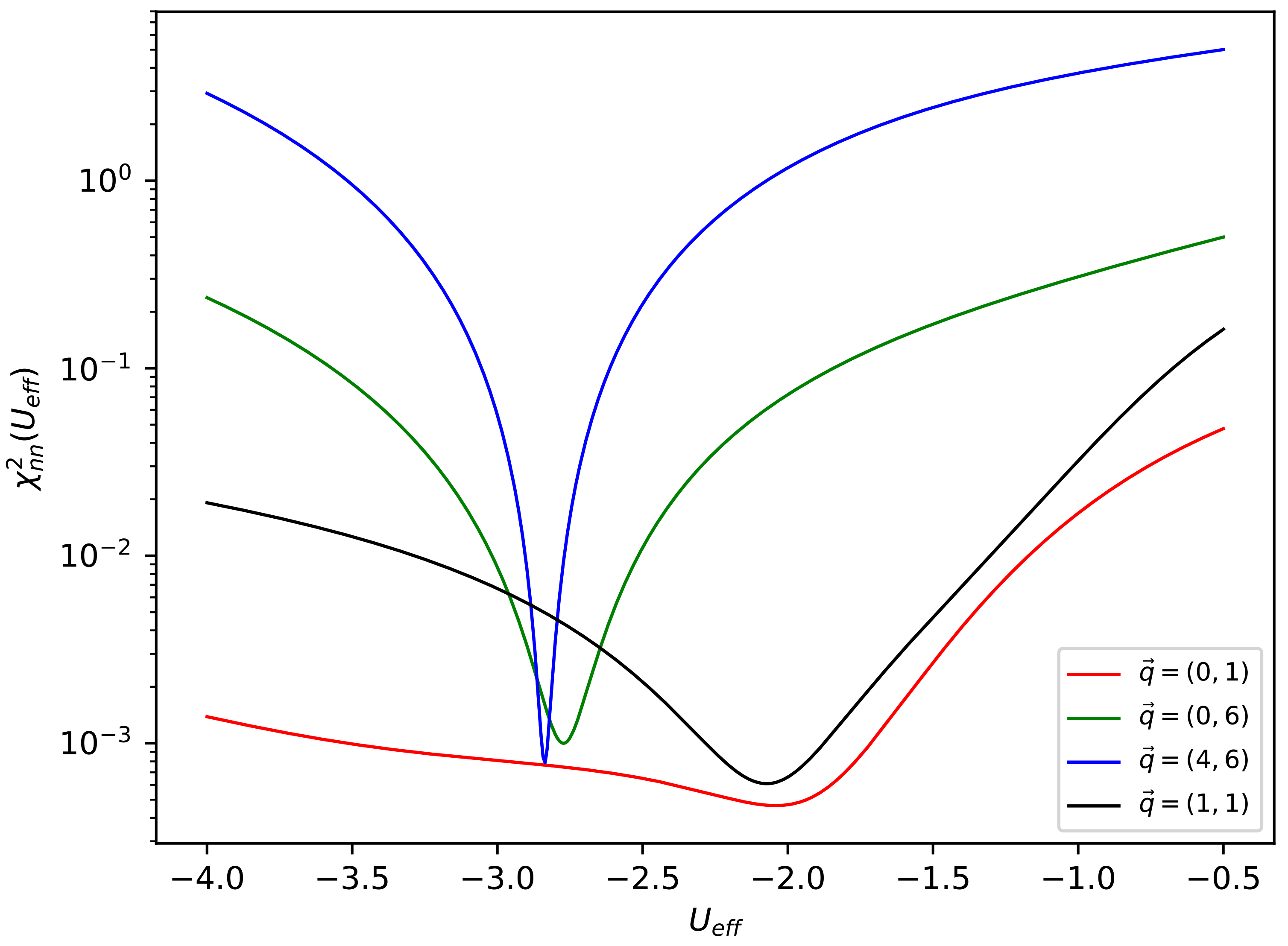
Our idea was to find that value of $U_{eff}$ used in GRPA that minimized the disagreement with the AFQMC imaginary time results, for a given momentum. To accomplish this, we used a ${\chi }^2$ test to find the value of $U_{eff}$ that minimized this test. In other words, we sought to find the value of $U_{eff}$ that minimized the expression:

$${\chi }^2\left(U_{eff}\right)=\sum _{i=0}^N{\left[F_{nn}^{GRPA}(\mathbf{q},{\tau }_i;U_{eff})-F_{nn}^{AFQMC}(\mathbf{q},{\tau }_i)\right]}^2,$$

(19)

where N is the number of imaginary time instants used, the physical potential is $U=-4.0$, and the methodology used is indicated with a superscript.

Our results are given in Figure 3. We performed this calculation for the same momenta used to generate Figure 1. This yielded a set of effective potential values for each momenta that were then used in a second round of GRPA calculations. We present these results and our interpretations in the next section.

3.3. Accuracy of GRPA for Static and Dynamic Properties

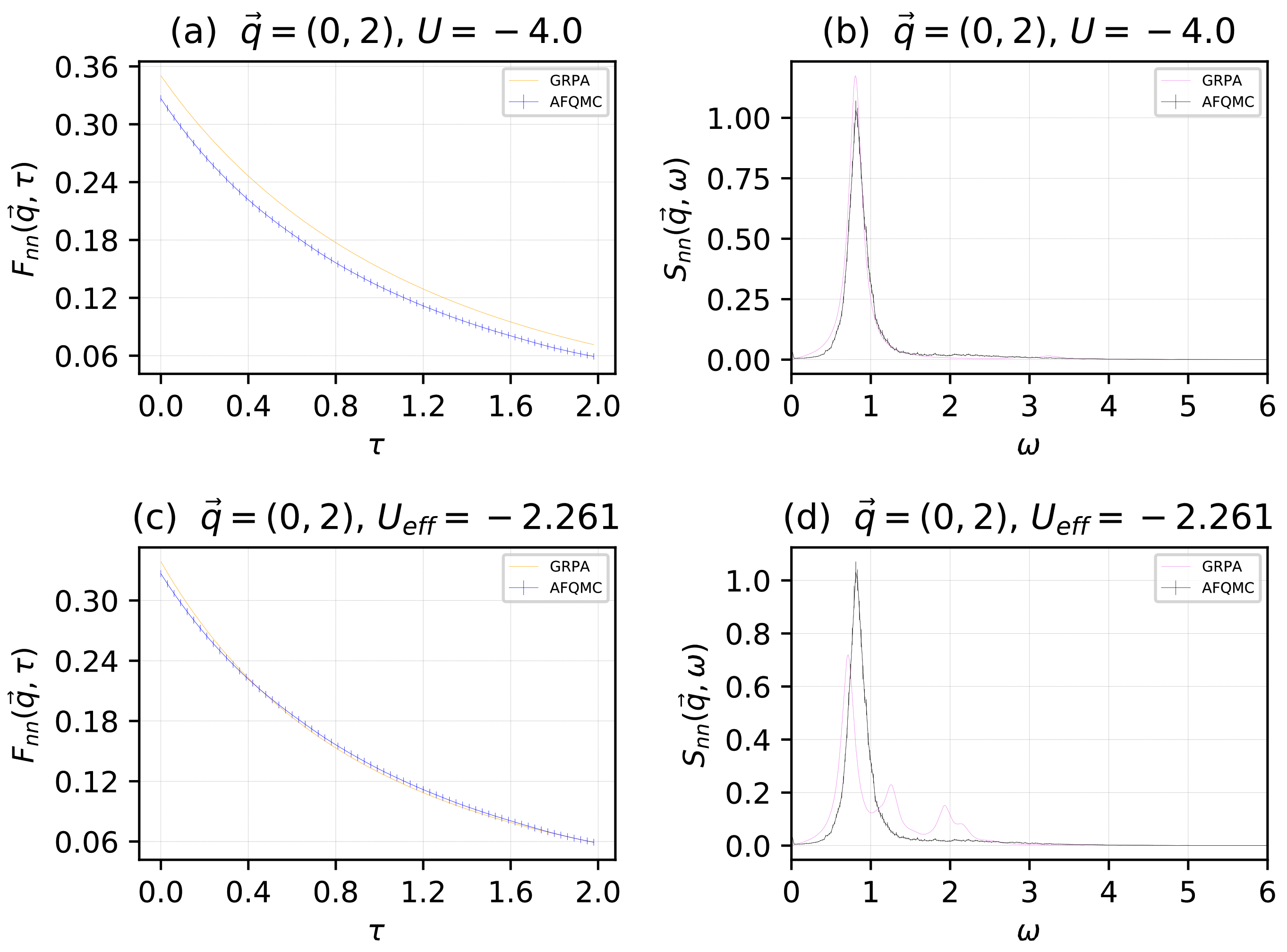
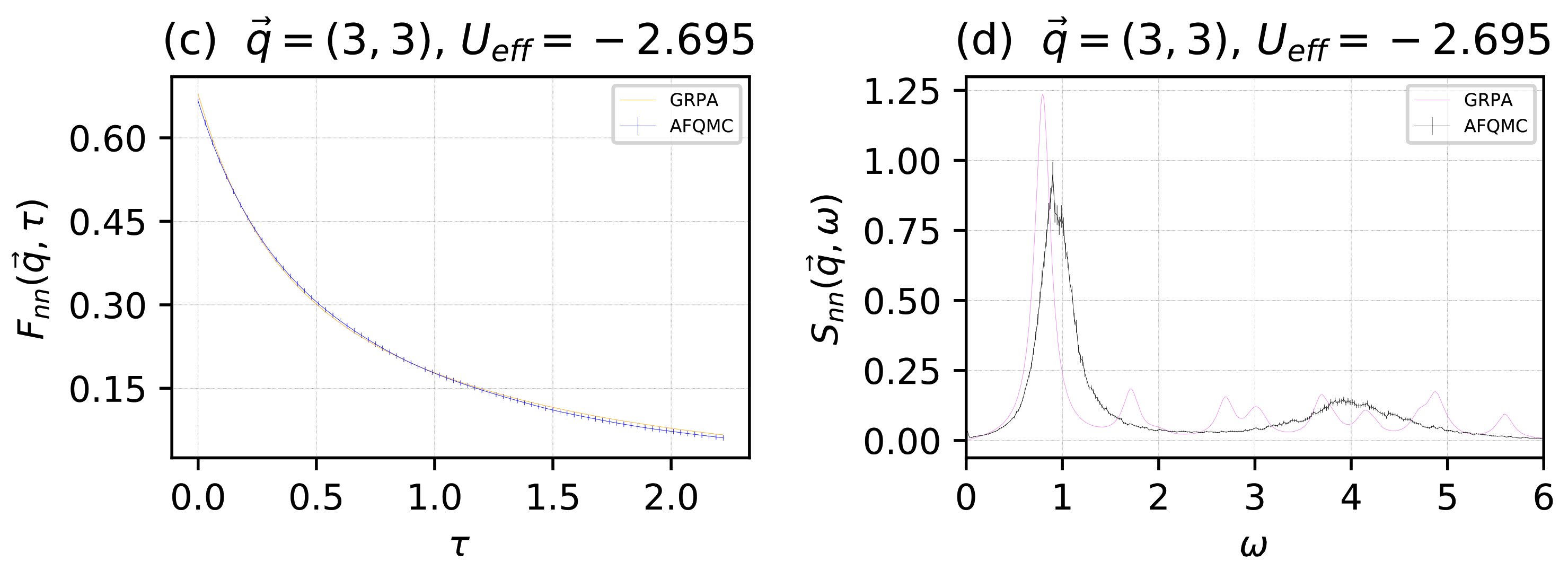
We now present a comparison between the real-time and imaginary-time results using the physical potential and the effective potential. The particle and lattice site numbers were the same as those used to generate Figure 1 and Figure 2. In Figure 4, we give results for the momenta value $\mathbf{q}=(0,2)$. In the top two sub-panels, we give results for $F_{nn}(\mathbf{q},\tau )$ and $S_{nn}(\mathbf{q},\omega )$, computed with AFQMC and GRPA, where the physical potential $U=-4.0$ was used in both methodologies. In the bottom two sub-panels, we give results for the same functions, but computed with AFQMC using the physical potential $U=-4.0$, and with GRPA using the effective potential $U_{eff}=-2.261$. In Figure 5, we followed the same procedure for the momenta value $\mathbf{q}=(3,3)$, using an effective potential $U_{eff}=-2.695$. We note that by minimizing the disagreement between the imaginary time correlation functions $F_{nn}^{QMC}(\mathbf{q},\tau )$ and $F_{nn}^{GRPA}(\mathbf{q},\tau )$ using an effective potential, we appear to obtain poorer results for the real-time correlation functions $S_{nn}^{QMC}(\mathbf{q},\omega )$ and $S_{nn}^{GRPA}(\mathbf{q},\omega )$. In Figure 4a,c and Figure 5a,c, blue indicates AFQMC data and orange indicates GRPA data. In Figure 4b,d and Figure 5b,d, black indicates AFQMC data, and violet indicates GRPA data.

We interpret these results using some relations from the theory of correlation functions. We start with:

$$G(\mathbf{r},\tau )=\frac{1}{2\pi }{\int }_{}^{}F(\mathbf{q},\tau )e^{i\mathbf{q}·\mathbf{r}}d\mathbf{q},$$

(20)

where $F(\mathbf{q},\tau )$ is the imaginary time, intermediate scattering function. $G(\mathbf{r},\tau )$ is the imaginary-time van Hove function, defined as:

$$G(\mathbf{r},\tau )=〈{\Psi }_0\left|e^{\tau \widehat{H}}{\widehat{n}}_{\mathbf{r}}{e}^{-\tau \widehat{H}}{\widehat{n}}_{\mathbf{0}}\right|{\Psi }_0〉,$$

(21)

where ${\widehat{n}}_{\mathbf{r}}$ is the space density operator at position $\mathbf{r}$ and imaginary time $\tau =0$ and ${\widehat{n}}_{\mathbf{0}}$ is the space density operator at position $\mathbf{r}=0$ and imaginary time $\tau =0$. The van Hove function is the spacial dynamical density autocorrelation function, as the intermediate scattering function is the momentum dynamical density autocorrelation function. Importantly, the van Hove function satisfies the relation [37]:

$$G(\mathbf{r},0)=\delta \left(\mathbf{r}\right)+\rho g\left(\mathbf{r}\right),$$

(22)

where $g\left(\mathbf{r}\right)$ is the radial distribution function, and $\rho =\frac{{\mathcal{N}}_p}{{\mathcal{N}}_s}$ is the number density of the system.

Using Equations (20) and (22), we see that Figure 4a and Figure 5a indicate that when we use the physical potential $U=-4.0$ in GRPA, there is a disagreement between AFQMC and GRPA in the static correlation functions, in this case $G_{nn}(\mathbf{r},0)$ which through (22), is proportional to $g_{nn}\left(\mathbf{r}\right)$, the density–density radial distribution function. When we use an effective potential $U_{eff}$ that minimizes the disagreement between $F_{nn}^{QMC}(\mathbf{q},\tau )$ and $F_{nn}^{GRPA}(\mathbf{q},\tau )$, we obtain better agreement for the static properties of the system but poorer agreement for the dynamical properties. Consequently, when one is only interested in finding static properties, it appears that an effective potential $U_{eff}$, obtained through some optimization procedure using a comparison with exact results, should be employed. When dynamical properties are needed, the physical potential U should be used.

We comment that an alternative method for finding an effective value of the interaction would be to find an effective potential that minimized the difference between the pairing gap calculated with AFQMC ($\Delta =0.73t$) [16] and the value calculated with GRPA. At the BCS level, we found that $U_{eff}=-2.75$ accomplishes this. This value is in reasonable agreement with the values we infer from Figure 3, in particular for the cases with momenta $\mathbf{q}=(0,6)$ and $\mathbf{q}=(4,6)$.

4. Conclusions and Future Directions

We studied a $2D$, attractive, cold Fermi gas, modeled with a Hubbard Hamiltonian. We compared the AFQMC and GRPA results for the imaginary time density and spin correlation functions. With the physical potential used in AFQMC, GRPA gave good results for the peak of the Goldstone mode collective excitation but gave poorer results for the static properties of the system. We outlined a procedure for systematically improving the results of GRPA for the static properties of our system using an effective potential. Though this procedure may improve the quality of the results for the static properties, it usually leads to poorer results for the dynamical properties. Our results indicate that for GRPA the physical potential should be used to obtain the dynamical correlations. If the static properties are desired, an effective potential can be used in GRPA to obtain better results for the static correlations.

Going forward, we plan to implement a more sophisticated mean-field scheme for approximating the states and generating the response functions for cold Fermi gases. One promising approach is to replace the BCS Hamiltonian in Equation (7) with a Hartree-Fock-Bogoliubov (HFB) Hamiltonian. The implementation of this methodology is considerably more involved because of the greater complexity of the HFB formalism. We are also interested in comparing AFQMC and GRPA results for cold Fermi gases in the dilute regime, where ${\mathcal{N}}_p<{\mathcal{N}}_s$, and in the spin-imbalanced regime, where ${\mathcal{N}}_{\uparrow }\ne {\mathcal{N}}_{\downarrow }$. Computational experiments and theoretical studies will allow us to assess the stability of the supersolid phase outside of the narrow half-filling, spin balanced regime.

References

- Giorgini, S.; Pitaevskii, L.P.; Stringari, S. Theory of ultracold atomic Fermi gases. Rev. Mod. Phys. 2008, 80, 1215–1274. [Google Scholar] [CrossRef] [Green Version]
- Bloch, I.; Dalibard, J.; Zwerger, W. Many-body physics with ultracold gases. Rev. Mod. Phys. 2008, 80, 885–964. [Google Scholar] [CrossRef] [Green Version]
- Gross, C.; Bloch, I. Quantum simulations with ultracold atoms in optical lattices. Science 2017, 357, 995–1001. [Google Scholar] [CrossRef] [PubMed] [Green Version]
- Rosenberg, P.; Shi, H.; Zhang, S. Ultracold Atoms in a Square Lattice with Spin-Orbit Coupling: Charge Order, Superfluidity, and Topological Signatures. Phys. Rev. Lett. 2017, 119, 265301. [Google Scholar] [CrossRef] [PubMed] [Green Version]
- Lin, Y.J.; Compton, R.L.; Jiménez-García, K.; Porto, J.V.; Spielman, I.B. Synthetic magnetic fields for ultracold neutral atoms. Nature 2009, 462, 628–632. [Google Scholar] [CrossRef] [PubMed] [Green Version]
- Carlson, J.; Gandolfi, S.; Gezerlis, A. Quantum Monte Carlo approaches to nuclear and atomic physics. Prog. Theor. Exp. Phys. 2012, 2012, 01A209. [Google Scholar] [CrossRef] [Green Version]
- van Wyk, P.; Tajima, H.; Inotani, D.; Ohnishi, A.; Ohashi, Y. Superfluid Fermi atomic gas as a quantum simulator for the study of the neutron-star equation of state in the low-density region. Phys. Rev. A 2018, 97, 013601. [Google Scholar] [CrossRef] [Green Version]
- Brown, P.T.; Mitra, D.; Guardado-Sanchez, E.; Nourafkan, R.; Reymbaut, A.; Hébert, C.D.; Bergeron, S.; Tremblay, A.M.S.; Kokalj, J.; Huse, D.A.; et al. Bad metallic transport in a cold atom Fermi-Hubbard system. Science 2019, 363, 379–382. [Google Scholar] [CrossRef] [Green Version]
- Zhang, D.W.; Zhu, Y.Q.; Zhao, Y.X.; Yan, H.; Zhu, S.L. Topological quantum matter with cold atoms. Adv. Phys. 2018, 67, 253–402. [Google Scholar] [CrossRef]
- Mitra, D.; Brown, P.T.; Guardado-Sanchez, E.; Kondov, S.S.; Devakul, T.; Huse, D.A.; Schauß, P.; Bakr, W.S. Quantum Gas Microscopy of an Attractive Fermi–Hubbard System. Nat. Phys. 2018, 14, 173–177. [Google Scholar] [CrossRef] [Green Version]
- Bulgac, A. Time-Dependent Density Functional Theory and the Real-Time Dynamics of Fermi Superfluids. Annu. Rev. Nucl. Part. Sci. 2013, 63, 97. [Google Scholar] [CrossRef] [Green Version]
- Ganesh, R.; Paramekanti, A.; Burkov, A.A. Collective modes and superflow instabilities of strongly correlated Fermi superfluids. Phys. Rev. A 2009, 80, 043612. [Google Scholar] [CrossRef] [Green Version]
- Yunomae, Y.; Yamamoto, D.; Danshita, I.; Yokoshi, N.; Tsuchiya, S. Instability of superfluid Fermi gases induced by a rotonlike density mode in optical lattices. Phys. Rev. A 2009, 80, 063627. [Google Scholar] [CrossRef] [Green Version]
- Zhao, H.; Gao, X.; Liang, W.; Zou, P.; Yuan, F. Dynamical structure factors of a two-dimensional Fermi superfluid within random phase approximation. New J. Phys. 2020, 22, 093012. [Google Scholar] [CrossRef]
- Vitali, E.; Shi, H.; Qin, M.; Zhang, S. Visualizing the BEC-BCS crossover in a two-dimensional Fermi gas: Pairing gaps and dynamical response functions from ab initio computations. Phys. Rev. A 2017, 96, 061601. [Google Scholar] [CrossRef] [Green Version]
- Vitali, E.; Kelly, P.; Lopez, A.; Bertaina, G.; Galli, D.E. Dynamical structure factor of a fermionic supersolid on an optical lattice. Phys. Rev. A 2020, 102, 053324. [Google Scholar] [CrossRef]
- Shi, H.; Chiesa, S.; Zhang, S. Ground-state properties of strongly interacting Fermi gases in two dimensions. Phys. Rev. A 2015, 92, 033603. [Google Scholar] [CrossRef] [Green Version]
- Bertaina, G.; Giorgini, S. BCS-BEC Crossover in a Two-Dimensional Fermi Gas. Phys. Rev. Lett. 2011, 106, 110403. [Google Scholar] [CrossRef] [Green Version]
- Vitali, E.; Shi, H.; Qin, M.; Zhang, S. Computation of dynamical correlation functions for many-fermion systems with auxiliary-field quantum Monte Carlo. Phys. Rev. B 2016, 94, 085140. [Google Scholar] [CrossRef] [Green Version]
- Hoinka, S.; Lingham, M.; Delehaye, M.; Vale, C.J. Dynamic Spin Response of a Strongly Interacting Fermi Gas. Phys. Rev. Lett. 2012, 109, 050403. [Google Scholar] [CrossRef]
- Zhang, S. Auxiliary-Field Quantum Monte Carlo for Correlated Electron Systems. In Emergent Phenomena in Correlated Matter: Modeling and Simulation; Pavarini, E., Koch, E., Schollwöck, U., Eds.; Verlag des Forschungszentrum: Jülich, Germany, 2013; Volume 3. [Google Scholar]
- Bertaina, G.; Galli, D.E.; Vitali, E. Statistical and computational intelligence approach to analytic continuation in Quantum Monte Carlo. Adv. Phys. X 2017, 2, 302–323. [Google Scholar] [CrossRef] [Green Version]
- Vitali, E.; Rossi, M.; Reatto, L.; Galli, D.E. Ab initio low-energy dynamics of superfluid and solid 4He. Phys. Rev. B 2010, 82, 174510. [Google Scholar] [CrossRef] [Green Version]
- Moskowitz, J.W.; Schmidt, K.E.; Lee, M.A.; Kalos, M.H. A new look at correlation energy in atomic and molecular systems. II. The application of the Green’s function Monte Carlo method to LiH. J. Chem. Phys. 1982, 77, 349–355. [Google Scholar] [CrossRef]
- Reynolds, P.J.; Ceperley, D.M.; Alder, B.J.; Lester, W.A. Fixed-node quantum Monte Carlo for molecules. J. Chem. Phys. 1982, 77, 5593–5603. [Google Scholar] [CrossRef]
- Varma, C.M. Higgs Boson in Superconductors. J. Low Temp. Phys. 2002, 126, 901–909. [Google Scholar] [CrossRef]
- Cea, T.; Castellani, C.; Seibold, G.; Benfatto, L. Nonrelativistic Dynamics of the Amplitude (Higgs) Mode in Superconductors. Phys. Rev. Lett. 2015, 115, 157002. [Google Scholar] [CrossRef]
- Podolsky, D.; Auerbach, A.; Arovas, D.P. Visibility of the amplitude (Higgs) mode in condensed matter. Phys. Rev. B 2011, 84, 174522. [Google Scholar] [CrossRef] [Green Version]
- Shimano, R.; Tsuji, N. Higgs Mode in Superconductors. Annu. Rev. Condens. Matter Phys. 2020, 11, 103–124. [Google Scholar] [CrossRef] [Green Version]
- Pekker, D.; Varma, C. Amplitude/Higgs Modes in Condensed Matter Physics. Annu. Rev. Condens. Matter Phys. 2015, 6, 269–297. [Google Scholar] [CrossRef] [Green Version]
- Saccani, S.; Moroni, S.; Boninsegni, M. Excitation Spectrum of a Supersolid. Phys. Rev. Lett. 2012, 108, 175301. [Google Scholar] [CrossRef] [PubMed] [Green Version]
- Saccani, S.; Moroni, S.; Vitali, E.; Boninsegni, M. Bose Soft Discs: A Minimal Model for Supersolidity. Mol. Phys. 2011, 109, 2807–2812. [Google Scholar] [CrossRef]
- Chomaz, L.; Petter, D.; Ilzhöfer, P.; Natale, G.; Trautmann, A.; Politi, C.; Durastante, G.; van Bijnen, R.M.W.; Patscheider, A.; Sohmen, M.; et al. Long-Lived and Transient Supersolid Behaviors in Dipolar Quantum Gases. Phys. Rev. X 2019, 9, 021012. [Google Scholar] [CrossRef] [Green Version]
- Natale, G.; van Bijnen, R.M.W.; Patscheider, A.; Petter, D.; Mark, M.J.; Chomaz, L.; Ferlaino, F. Excitation Spectrum of a Trapped Dipolar Supersolid and Its Experimental Evidence. Phys. Rev. Lett. 2019, 123, 050402. [Google Scholar] [CrossRef] [Green Version]
- Guo, M.; Böttcher, F.; Hertkorn, J.; Schmidt, J.N.; Wenzel, M.; Büchler, H.P.; Langen, T.; Pfau, T. The Low-Energy Goldstone Mode in a Trapped Dipolar Supersolid. Nature 2019, 574, 386–389. [Google Scholar] [CrossRef] [Green Version]
- Tanzi, L.; Roccuzzo, S.M.; Lucioni, E.; Famà, F.; Fioretti, A.; Gabbanini, C.; Modugno, G.; Recati, A.; Stringari, S. Supersolid Symmetry Breaking from Compressional Oscillations in a Dipolar Quantum Gas. Nature 2019, 574, 382–385. [Google Scholar] [CrossRef] [Green Version]
- Hansen, J.P.; McDonald, I.R. (Eds.) Chapter 7—Time-dependent Correlation and Response Functions. In Theory of Simple Liquids, 4th ed.; Academic Press: Oxford, UK, 2013; pp. 265–310. [Google Scholar] [CrossRef]
Figure 1.
The density–density imaginary time intermediate scattering function (main sub-panel), and corresponding density–density dynamical structure factor (inset), for the momenta: (a), (b), (c), (d), in units of . Blue indicates AFQMC data and orange indicates GRPA data.
Figure 2.
The spin–spin imaginary time intermediate scattering function (main sub-panel), and corresponding spin–spin dynamical structure factor (inset), for the momenta: (a), (b), (c), (d), in units of . Green indicates AFQMC data and red indicates GRPA data.
Figure 3.
, the chi-squared factor comparing the AFQMC and GRPA results for the density–density intermediate scattering function, expressed as a function of the effective potential . Results are given for the momenta used in Figure 1.
Figure 4.
For momenta , in units of : The density–density, imaginary-time intermediate scattering function for the physical potential (a). The density–density dynamical structure factor for the physical potential (b). The density–density, imaginary-time intermediate scattering function for the renormalized, effective potential (c). The density–density dynamical structure factor for the renormalized, effective potential (d). In the left sub-panels, blue indicates AFQMC data and orange indicates GRPA data. In the right sub-panels, black indicates AFQMC data and violet indicates GRPA data.
Figure 5.
For momenta , in units of : The density–density, imaginary-time intermediate scattering function for the physical potential (a). The density–density dynamical structure factor for the physical potential (b). The density–density, imaginary time intermediate scattering function for the renormalized, effective potential (c). The density–density dynamical structure factor for the renormalized, effective potential (d). In the left sub-panels, blue indicates AFQMC data and orange indicates GRPA data. In the right sub-panels, black indicates AFQMC data and violet indicates GRPA data.
Publisher’s Note: MDPI stays neutral with regard to jurisdictional claims in published maps and institutional affiliations. |
© 2021 by the authors. Licensee MDPI, Basel, Switzerland. This article is an open access article distributed under the terms and conditions of the Creative Commons Attribution (CC BY) license (https://creativecommons.org/licenses/by/4.0/).
Share and Cite
MDPI and ACS Style
Kelly, P.; Vitali, E. On the Accuracy of Random Phase Approximation for Dynamical Structure Factors in Cold Atomic Gases. Atoms 2021, 9, 88. https://0-doi-org.brum.beds.ac.uk/10.3390/atoms9040088
AMA Style
Kelly P, Vitali E. On the Accuracy of Random Phase Approximation for Dynamical Structure Factors in Cold Atomic Gases. Atoms. 2021; 9(4):88. https://0-doi-org.brum.beds.ac.uk/10.3390/atoms9040088
Chicago/Turabian StyleKelly, Patrick, and Ettore Vitali. 2021. "On the Accuracy of Random Phase Approximation for Dynamical Structure Factors in Cold Atomic Gases" Atoms 9, no. 4: 88. https://0-doi-org.brum.beds.ac.uk/10.3390/atoms9040088
Note that from the first issue of 2016, this journal uses article numbers instead of page numbers. See further details here.