Monocular Visual Inertial Direct SLAM with Robust Scale Estimation for Ground Robots/Vehicles

1
Mechanical & Mechatronincs Engineering Department, University of Waterloo, Waterloo, ON N2L 3G1, Canada
2
School of Engineering, University of Guelph, Guelph, ON N1G 2W1, Canada
*
Author to whom correspondence should be addressed.
Robotics 2021, 10(1), 23; https://0-doi-org.brum.beds.ac.uk/10.3390/robotics10010023
Submission received: 21 November 2020
/
Revised: 5 January 2021
/
Accepted: 8 January 2021
/
Published: 26 January 2021
(This article belongs to the Section Agricultural and Field Robotics)
Abstract
:In this paper, we present a novel method for visual-inertial odometry for land vehicles. Our technique is robust to unintended, but unavoidable bumps, encountered when an off-road land vehicle traverses over potholes, speed-bumps or general change in terrain. In contrast to tightly-coupled methods for visual-inertial odometry, we split the joint visual and inertial residuals into two separate steps and perform the inertial optimization after the direct-visual alignment step. We utilize all visual and geometric information encoded in a keyframe by including the inverse-depth variances in our optimization objective, making our method a direct approach. The primary contribution of our work is the use of epipolar constraints, computed from a direct-image alignment, to correct pose prediction obtained by integrating IMU measurements, while simultaneously building a semi-dense map of the environment in real-time. Through experiments, both indoor and outdoor, we show that our method is robust to sudden spikes in inertial measurements while achieving better accuracy than the state-of-the art direct, tightly-coupled visual-inertial fusion method.
1. Introduction
Over the past few years, Simultaneous Localization and Mapping (SLAM) has become an established technique for motion estimation of autonomous robots. SLAM utilizes information from two or more sensors (such as IMU, GPS, Camera, Laser Scanners etc.) to estimate the robot-pose as well as features in the environment at the current time step, using the measurements from just the last time step (filtering), or past few time steps (smoothing).
For environments when GPS cannot be used, for example indoor, using vision system is a great alternative [1,2]. Over the past decade, researchers have developed techniques for camera-only odometry as well as environment reconstruction. However, due to the absence of metric information, monocular (single camera) SLAM is only up-to scale. Moreover, in the presence of predominant rotational movements, monocular SLAM methods usually fail due to insufficient epipolar stereo-correspondences.
Inertial Measurement Units (IMUs) provide both metric information and rotation estimates. However, developing dead-reckoning methods using an IMU as the only sensor, is infeasible as errors in pose estimation quickly accumulate and grow out of bounds. IMUs are cheap and almost always present in modern camera phones. The two sensors, an IMU and a monocular camera, complement each other well by addressing each other’s short-comings; IMU provides the missing scale and rotation information while the camera helps in keeping IMU errors within acceptable bounds. For this reason, camera–IMU fusion techniques have been developed [3] and deployed in applications such as robotics [4] and augmented/virtual reality (AR/VR) [5].
However, monocular visual-inertial fusion techniques have been limited to key-point based methods which build sparse environment maps, and when used with autonomous systems they need to rely on other sensors, such as laser scanners and sonars, to extract useful information about the environment for critical tasks such as navigation. Recently, direct methods have been developed that build richer and more visually informative semi-dense maps in real-time, providing promising prospects for navigation using only visual and inertial sensors. More recently, the so-called tightly-coupled approaches for visual-inertial fusion, developed originally for key-point based methods, have been extended for the direct visual SLAM framework. However, the joint optimization framework, used in the tight-coupled technique, degrades when the measurements from IMU are affected by sudden, unexpected spikes encountered when deployed on a land-vehicle traversing over bumps, pot-holes or general change in terrain.
In this paper, we present a novel direct semi-tightly coupled visual-inertial fusion technique which is robust in presence of sudden, unintended spikes in IMU measurements experienced when the camera–IMU platform is mounted on a land-vehicle traversing a bumpy terrain. The primary contribution of our work is the the development of an optimization framework that enforces epipolar constraints to correct pose priors, obtained by integrating noisy IMU measurements, while taking into account geometric misalignment arising due to direct visual optimization. To the best of our knowledge, our work is the first to handle sudden spikes in IMU measurements in a direct visual-inertial framework.
We start by discussing relevant work in Section 2, followed by brief mathematical preliminaries in Section 3. We provide a background on direct state estimation techniques in Section 4 followed by a detailed description of our methodology in Section 5, experiments in Section 6 and results in Section 7. We finally conclude the paper in Section 8 by highlighting the limitations and providing directions for future work.
2. Related Work
Our approach for visual-inertial data fusion builds upon the existing frameworks for direct monocular visual SLAM. We start by discussing relevant research on vision-only SLAM to justify our design choices, followed by recent work on visual-inertial SLAM.
2.1. Monocular-Vision Only SLAM
Although stereo-based techniques for visual odometry have existed for quite sometime, MonoSLAM [6] laid the foundation for monocular visual SLAM, where an Extended Kalman Filter (EKF) based algorithm was used to track and map a few key-points. The inverse-depth parameterization introduced in Reference [7] made it possible to represent depths of points from unity to infinity. The measurement model, along with its EKF update rule, is almost universally used in visual SLAM techniques.
Parallel Tracking and Mapping (PTAM) [8] introduced the concept of parallelizing tracking and mapping on separate cores on the same CPU, paving way for real-time applications. Dense Tracking and Mapping (DTAM) [9] introduced the concept of “direct-tracking” and built a dense environment reconstruction by utilizing the parallel architecture of a GPU. Since then, References [10,11,12] have taken advantage of parallel GPU architecture and 3D point cloud stitching using Iterative Closet Point (ICP) algorithm to achieve impressive results. However, such methods require the use of GPU and depth cameras which make them infeasible for real-time implementation on resource constrained systems.
In Reference [3], the authors have used second order splines for real-time estimation of the absolute scale and subsequently an EKF to predict the 3D pose. However, the method is loosely coupled and was developed for key-point based visual SLAM framework, PTAM. In their paper, a weighing term allows them to rely more on the inertial measurements during bad visual tracking. Since it is difficult to predict sudden spikes in IMU measurements beforehand, it would be difficult to select an appropriate weighing term in favour of visual measurements. In contrast, our approach includes the visual-inertial fusion to predict the optimized 3D pose in the tracking thread itself. Moreover, the inclusion of epipolar constraint in our tracking step, enables us to maintain good stereo-correspondences in each frame.
The work of Reference [13] builds upon Reference [8] to fuse inertial information using a variant of EKF. The tracking accuracy was further improved in Reference [14] and later in Reference [15] by developing a SLAM framework, complete with loop closure and re-localization to achieve long term stability. However, such techniques use key-point descriptors to first isolate a subset of pixels, which not only demand computational overhead but also result in loss of rich visual information by building only a sparse representation of the environment.
Direct Tracking and Mapping introduced in Reference [9] was used in Reference [16] to perform visual SLAM on gradient-rich image regions to generate a much denser environment reconstruction. This approach avoids costly key point computations and generates a denser map in real-time. This approach was further extended to omnidirectional [17] and stereo [18] and was later augmented with pose-graph optimization [19] using the technique of Reference [20] to show very accurate results. Dense Piecewise Planar Tracing and Mapping (DPPTAM) [21] used the concept of super-pixels [22], to build an even denser map of the environment, under the assumption that neighbouring pixels with similar intensity are likely to lie on one plane. Unlike Reference [21], Multi-level Mapping [23] used a K-D tree to generate almost fully dense reconstruction. In contrast, Reference [24] further sparsifies high-gradient pixels by extracting corners to achieve fast tracking while compromising the reconstruction density. Our method finds a middle ground and builds upon Reference [19] to achieve real-time results while not sacrificing computational overhead required for dense reconstructions as in References [21,23] or not losing out on the density reconstructed environment as in Reference [24]. However, since the core visual-tracking methodology is similar in all of these approaches, our method can be easily adapted to achieve trade-offs in either direction; to build dense maps or implement faster tracking.
2.2. Visual-Inertial Fusion
Although visual-inertial fusion techniques have been of interest to researchers for over a decade, the work of Ref. [25] stands out. In this work, a state vector with current and last few poses are augmented with landmark poses in the current field of view and jointly updated using an Extended Kalman Filter (EKF). Ref. [26] is an extension of Ref. [25] that is twice as fast. The gain in computational speed is a result of efficient representation of the Hessian matrix in its inverse square root form, such that quick single-precision operations can performed. This representation has enabled [26] to be deployed in real-time resource constrained embedded systems. Recently, Ref. [27] proposed a method of on-the-fly scale estimation and camera–IMU extrinsic calibration but this method is based on sparse key points. As the number of landmark poses in direct-methods is significantly larger than key-point methods, an equivalent extension of Refs. [25,26] or Ref. [27] results in significant computational overhead.
In contrast, inertial-aided direct visual methods have been proposed only recently. In Ref. [28], a method is described for unifying multiple IMU measurements into a single factor and sparse landmark features in a structureless approach in a factor-graph [29] framework. However, since the method is sparse and includes features only in a key-frame, it does not scale up for direct-methods. Ref. [30] describes a method for joint optimization of inertial and visual residuals (tightly-coupled) in real-time. However, we noticed in our experiments that in the presence of sudden spikes in IMU measurements, its performance degrades. Further, random initialization of inverse-depth renders the joint optimization step sub-optimal. Epipolar constraints were exploited for aligning feature points with ground-truth epipolar lines in a joint frame-work in Ref. [31]. However, the technique is sparse and relies on extraction of feature correspondences.
In our work, we present a novel visual-inertial technique by formulating epipolar constraints in a direct-image alignment framework, in contrast to sparse formulations such as in Ref. [31]. Within our inertial-epipolar optimization technique, we include each pixel’s inverse depth variance and account for visual misalignment, to correct noisy pose prior obtained from integration of IMU measurements. By isolating inertial terms from a joint framework and performing inertial-epipolar optimization after direct-visual alignment, our method is able to tackle sudden, spurious spikes in IMU measurements. To the best of our knowledge, this problem has not been addressed in literature. In the experimental section, we compare our work with the state-of-the-art direct visual-inertial method [30] to demonstrate the robustness and accuracy of our technique, in presence of sudden bumps experienced by the camera–IMU platform, when mounted a moving land-vehicle. Further, due to the increased accuracy in pose-prediction, our method can be used to build a consistent semi-dense map of the environment.
In the next section, we briefly describe some preliminary concepts used in visual-inertial state estimation.
3. Preliminaries
3.1. Lie Group and Lie Algebra
The Lie Group is used to represent transformations and poses which encode the rotation as a rotation matrix and translation . Lie Algebra is the tangent space to the manifold at identity. The tangent space for the group is denoted by which coincides with the space of 3 × 3 skew symmetric matrices [28]. Every skew symmetric matrix can be identified with a vector in using the hat operator, :
where is a vector (in ), and , , are its components. Similarly, we map a skew symmetric matrix to a vector in using the vee operator : for a skew symmetric matrix , the vee operator is such that .
The exponential map at identity associates elements of the Lie Algebra to a rotation:
The logarithm map (at identity) associates a matrix ∈ to a skew symmetric matrix:
It is also worthwhile to note that =a, where a and are the rotation axes and the rotation angle of .
The use lie algebra in optimization allows for smooth pose updates which obey the properties of manifold operations.
3.2. IMU Model
Let represent the rotation, denote the translation vector and denote the velocity vector in the current frame j wrt the world reference frame w. This is calculated from the previous frame i by forward Euler integration as done in Reference [30];
where denotes the relative rotations between frames i and j, is the incremental velocity and is the translation vector. These variables are computed from the IMU measurements angular velocity, , and linear acceleration, , with biases and , respectively. The increments can be written in terms of measurements as:
where encodes the gravity vector and p denotes the instances where IMU measurements are available in between two camera frames i and j. The IMU biases are modelled as random walk processes with variances and :
3.3. Gravity Alignment
In order to obtain a correctly oriented world-frame map, we perform gravity alignment as an initialization step. We record a few IMU acceleration samples to estimate the initial World frame to Body Frame orientation (). First, we compute the magnitude of the gravity vector as:
We then compute the initial pitch and roll angles as:
where are the averaged accelerations over the first few frames in the Cartesian directions. As the yaw is undetermined from the accelerations alone, we assume initial yaw to be zero. In the presence of a magnetometer, better initialization to the yaw angle can be performed.
3.4. The State Vector
To aid in the estimation process, a state vector maintains the pose estimates, the updates on velocity and bias estimates. More specifically, the state is defined as where is a vector containing the bias in the 3D acceleration and 3D angular velocity measurements of the IMU. The pose element, , encodes the translation and and .
Our state-vector does not maintain the past states or feature positions unlike feature-based fusion methods due to the following reasons: (1) number of points in dense optimization methods is much more than feature-based methods and including them in the state adds significantly to the size and computational efficiency and (2) We follow a filtering based approach over the smoothing approach. The prior to our optimization is obtained by forward Euler integration described in Section 3.2. Once an estimate of the pose is obtained using method described in Section 5.1, the state vector is updated and used again for the next time step.
4. Background
4.1. Lucas-Kannade Image Alignment
This technique seeks to minimize the photometric residual with an objective function defined as:
where is the coordinate of a pixel in the template image , is a warp function that maps the pixel to its corresponding location in the target image . The goal of the optimization is to seek optimal parameters such that the cost, defined in Equation (15), is minimized for a small patch of pixels around the original pixel, .
4.2. Direct Image Alignment
This technique is a variant of the Lucas Kannade algorithm [32], where the warp function encodes unprojection of a pixel with an inverse depth and reprojected back on to the target image, after applying transformation to the unprojected point. More recently, this method has been applied to visual odometry applications [19,21,24], yielding impressive results. Here, instead of computing feature points, all pixels with a valid depth estimate (belonging to an inverse-depth map ) and having enough intensity gradient are included in a single objective function and the sum of squared intensity residuals is minimized.
where is the transformation encoding the rotation and translation and is the camera calibration matrix.
The formulation of the warp parameters as members of Lie Group allows for smooth updates in the tangent space . The minimum is calculated using variants of Gauss-Newton algorithm with increments as:
where is the stacked jacobain of all pixels for the residual, , with respect to the six elements of Lie Algebra .
It is worth noting here that the cost function (17) is highly non-linear. Further, in a monocular visual odometry setting, a random inverse depth map is assigned to bootstrap the process. Although, a robust weighing function, such as Huber [33] or Tukey, is deployed to handle outliers, improper initialization of initial Transformation estimate, , can force the optimization to converge to a local minima.
4.3. Visual Inertial Direct Odometry
This technique adds an IMU to aid in the optimization process. The best results have been achieved by ‘tightly-coupled’ approach, where the photometric residual (17) is jointly optimized along with an inertial-residual given by:
where denotes retraction from Lie Group to Lie algebra , is obtained by integrating IMU measurements from time frame i to j. denotes world frame of reference. is the state at the previous time frame i and is the parameter to be optimized. denote the rotation, translation, linear velocity, accelerometer bias and gyroscope bias, respectively.
Notice that the residual is minimized when the predicted state parameters match with the ones obtained from IMU measurements. In a joint estimation framework, where both and are minimized simultaneously, the updates in IMU pose, , is calculated first and used to “guide” the optimization of the photometric residual. This is typically desirable as the measurements from IMU provide both the initial estimate (by distorting the cost function to generate a new minima around the minima of the IMU residual) and a direction for convergence (through Jacobians of IMU residual with respect to photometric updates [30]). However, in presence of unexpected but unavoidable bumps, the new minima for this residual is highly offsetted from where it is desired. Since the original cost function (17) is highly non-linear, such an offset makes it susceptible to local minima.
In the next section, we address this issue by formulating a novel cost function where the inertial residual is separated out and correction is applied after the visual cost has been minimized, by imposing epipolar constraints.
5. Methodology
5.1. Visual-Inertial Epipolar Constrained Odometry
In this novel formulation, we decouple the IMU residuals from the direct visual image alignment step (17), where we first let photometric cost function converge with respect to the randomly initialized unscaled inverse depth map. After convergence, all the corresponding points on the target image are not perfectly aligned (but only a subset, the ones which satisfy the brightness consistency assumption). For the sake of simplicity, we assume that the optimization yields perfect matches (). We relax this assumption later in Section 5.2. Figure 1 shows the algorithm for visual inertial epipolar constrained odometry.
Using the prior transformation (described in Section 3.4) (), for each pixel in the key-frame image, we can construct an initial estimate for the epipolar line, () through the relation:
where is the initial estimated guess for the Fundamental Matrix constructed through which encodes and , and is the homogenized pixel coordinate . Using (20), we define the epipolar residual,
where is the function computing the euclidean distance between point, and line, .
The error function during the search along the epipolar line is shown in Section 5.3 in which the SSD Error is short for Sum of Squared difference Error.
The epipolar constraint dictates that the best match pixel () corresponding to the source pixel () must lie on the corresponding epipolar line (). We aim to obtain the optimal transformation () by applying updates to (obtained by integrating IMU measurements), such that the perpendicular distance between the epipolar line () and (corresponding point on target image after convergence of (17)) on the 2D image plane is minimized. We call this step “epipolar image alignment”. Our objective is two-fold: (1) to find so that 1D stereo-search along this line would give and (2) to obtain as a result of this alignment.
Note however, that this alignment is 2D and the rank of Fundamental Matrix is 2 which causes a loss of the scale information. This phenomenon can be imagined as “zooming in/out” on a scene where there is perfect 2D epipolar alignment but absence of scale information makes estimation of “zooming in/out” motion impossible.
To address this shortcoming, we formulate an inverse-depth residual to counter any scale drift during the epipolar optimization. We first estimate the initial scale by obtaining a coarse estimate of inverse depths for all pixels due to the transformation . This is done by finding , which is the perpendicular projection of on . The ratio of mean of all such inverse depths to the mean of our initial inverse depth assumption gives a good initial scale estimate. This process of finding scale is inspired by [19] where mean inverse depth is conserved to unity at each keyframe to prevent scale drift.
To conserve the scale drift during epipolar alignment, the following residual is formulated.
where, is the initial estimate of the inverse depth of pixel i obtained as explained above, is the third row of the incremental Rotation update, denotes dot product and is the incremental update in the translation ‘z’ direction.
Our complete cost function becomes:
where is the function computing the euclidean distance between point, and line, .
At this point, one might observe that the inverse depth residual is zero at the start and progressively grows with iteration. This effect is desirable and intended to counter the scale drift as it becomes more and more prominent during minimization of epipolar residual. The image of the epipole of the second image on the template (keyframe) image during the optimization process is shown in Figure 2.
5.2. Robust Weighing
Earlier in Section 5.1, we assumed perfect alignment of pixels as a result of the visual-inertial optimization step. However, due to random initialization at the start and general noise in camera pixel measurements, this assumption is not valid. In fact, only a subset of these pixels ‘align’ themselves well. The extent of alignment dictates the extent of relaxation allowed for a particular pixel in the epipolar alignment step (Section 5.1). In this section, we model the extent of this alignment by normalizing the epipolar and the inverse depth residuals Equation (26). In addition we employ robust weighting function to counter the effect of outliers.
Epipolar residuals for each pixel are normalized as follows:
where is the inverse depth variance, is the jacobian of the epipolar residual with respect to the inverse depth and is the camera pixel noise.
Similarly, inverse depth residual is normalized
where is the jacobian of the inverse depth residual with respect to the inverse depth.
We apply a single Huber weighing function to both the residuals given that if one pixel is an outlier, both the residuals must be weighed less.
5.3. Mapping
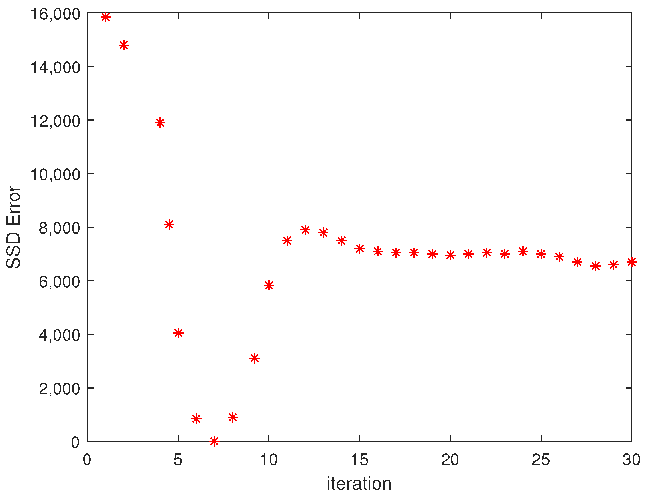
To enable real-time operation, both the Tracking and Mapping modules are implemented in parallel threads. The mapping thread is blocked until the image is first tracked and has a valid pose (), as depicted in Figure 1. We transform each valid pixel in the “keyframe” image (static for comparison with incoming image sequences and the image to which inverse-depth map is assigned) on to a corresponding pixel in the successive “reference” image (each incoming image) and perform a one-dimensional search along five equidistant points along the epipolar lines in both images (See Figure 3). Each successful stereo-match is at the point where the Sum of Squared Difference (SSD) error is minimum (See Figure 4) and corresponds to the best estimate of the original pixel in the keyframe image (shown as box in Figure 3) on corresponding reference image.
We follow a similar methodology to Reference [16] and employ geometric and photometric errors in the stereo computations as briefly described below. The reader is encouraged to refer to Reference [16] for details.
with;
where;
| : | camera-pixel noise |
| : | variance of positioning error of the initial |
| point on epipolar line | |
| : | gradient along the epipolar line |
| g: | normalized image gradient |
Following each successful stereo observation, the depth and variance is updated as:
where is the prior distribution and is the observed distribution.
6. Experiments
6.1. Setup
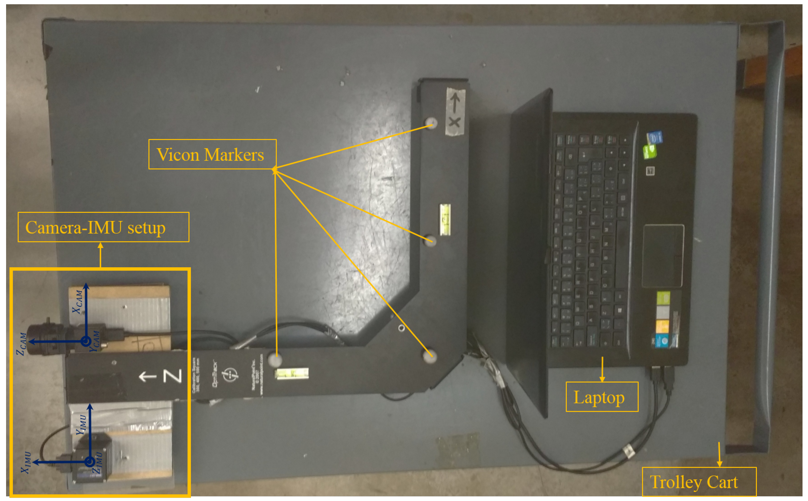
The experimental setup consist of a monocular camera (Flir PointGrey BlackFly @50fps from Flir) with a wide field of view (FOV) lens (90 to capture 640 × 480 monochrome images, and IMU (3DGX2 @100Hz from Microstrain) shown in Figure 5 to capture 6-dof linear accelerations and angular velocity. Both of these sensors were rigidly fixed on a base as shown in Figure 6. The processor used is a Lenovo Z40 laptop equipped with Intel i5 processor and 4GB of RAM, running Ubuntu Linux pre-loaded with Robot Operating System (ROS). Additionally, a Vicon Motion Capture System is used as Ground Truth for indoor experiments.
To highlight the advantages of our method, it was essential to have a set-up that could impart sudden unintentional bumps during movement. To realize that, a makeshift trolley-cart with one misaligned wheel, was used to impart sudden bumps to the set-up. Moreover, the inability to intentionally control the timing, duration or nature of sudden spikes in IMU measurements, makes our system mimic real world outdoor conditions where land-vehicles would encounter sudden bumps or change in terrain.
For outdoor experiments, the camera–IMU platform was mounted at the front-end of an off-road 6 × 6 vehicle, manufactured by ARGO, shown in Figure 7.
6.2. Calibration
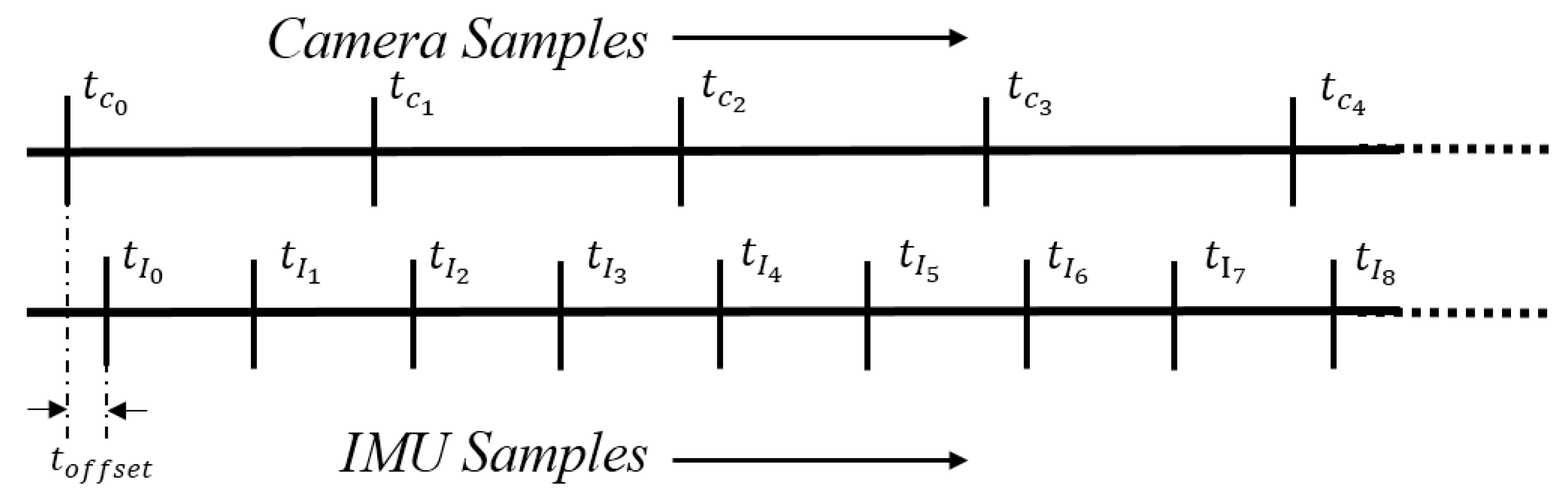
Before the start of the experiment, the camera–IMU system was calibrated offline in order to determine the focal lengths () and camera centre in pixels (), radial distortion parameters, the IMU-variances (using Allan Variance Analysis), IMU biases (), camera–IMU transformation matrix () and temporal offsets (time lag between each apparently overlapping camera and IMU sample (See Figure 8). The open-source package [34] was used to perform this calibration. Since we use a large FOV camera, the radial distortion due to lens was corrected for each incoming image using the distortion model available in the open-source undistorted package inside PTAM [8]. The equations described in Section 5 assume a pre-rectified image, free from radial distortion. The calibration parameters for our camera are shown in Table 1:
7. Results
In this section, we outline the results obtained both indoors and outdoors. We first perform experiments indoors where ground-truth was available and later do a qualitative evaluation in an outdoor setting.
7.1. Indoor Environment
7.1.1. Vicon Room
We analyse the accuracy of our algorithm and the tightly coupled approach in the presence of ground-truth data. The camera–IMU setup was mounted on a trolley with one misaligned wheel which produced unpredictable bumps during movement. To ensure the same conditions for both algorithms, Visual-Inertial Direct (abbreviated as VID) and our method (abbreviated as VIE), were initialized with the same random inverse depth map and the accuracy was analysed with reference to only one fixed key-frame. Note that the primary motive of our experiment was to observe the initial errors which, in the absence of loop-closure or pose-graph optimization, persist and accumulate throughout the experiment.
Since our long term objective was to develop this system for land-vehicles, the movement was limited to the two-dimensional plane only. Moreover, complex 3D trajectories are usually observed when mounted on drones or simply handheld mapping systems, where the noise profile due to wind-gusts or hand tremor is much different than what is observed in land-vehicles.
The platform was moved several times in presence of ground-truth in different directions and the results (RMSE errors) are summarized in Table 2.
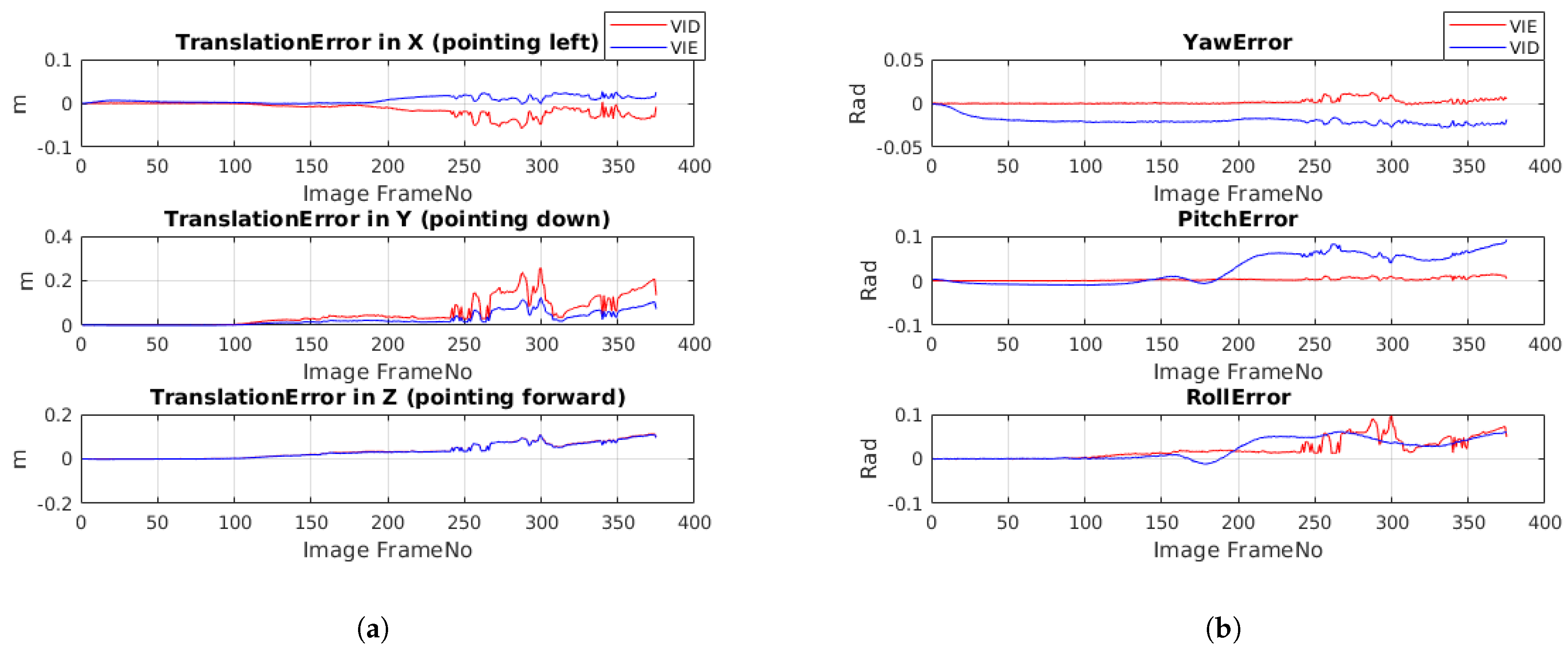
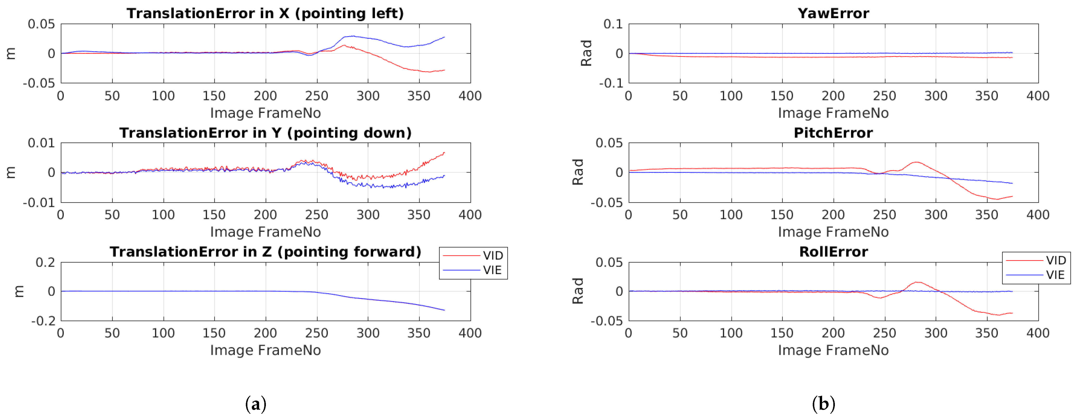
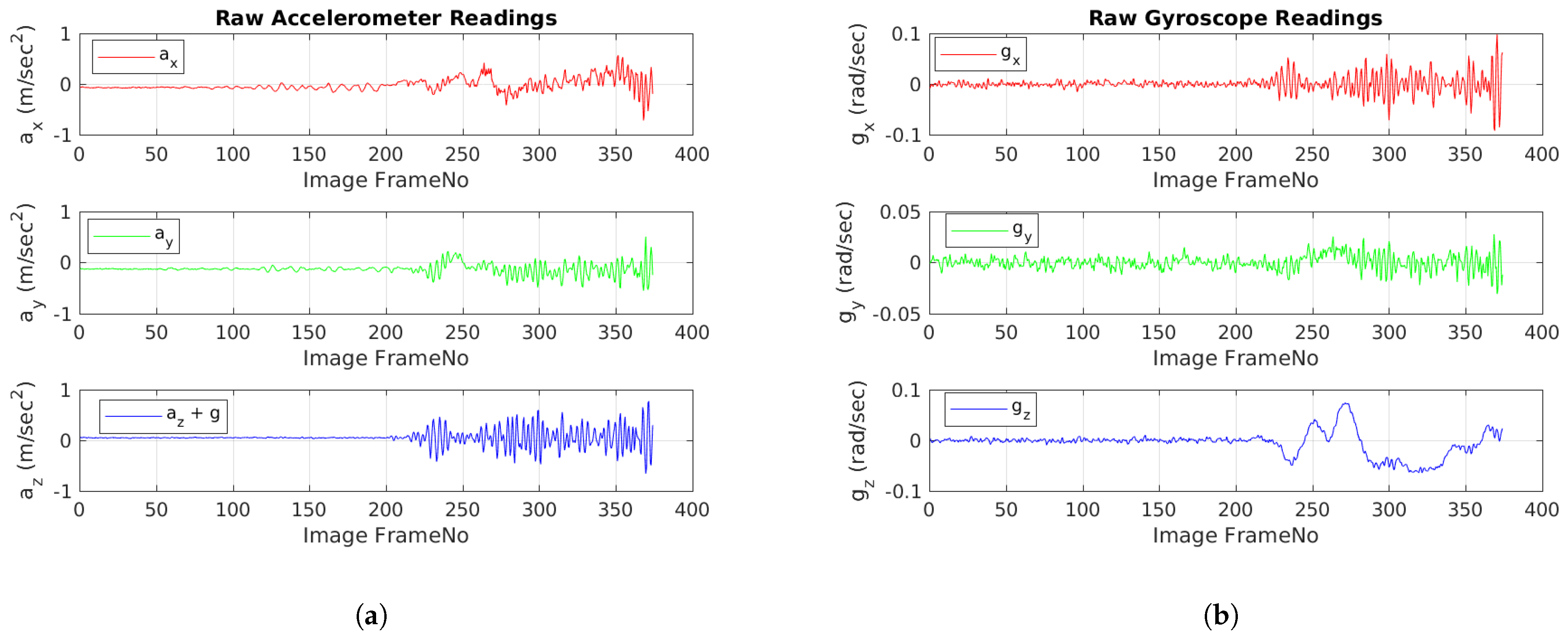
On closer inspection of the results in Table 2, one can observe that overall, our method achieves better accuracy than the state-of-the-art (~26% improvement in translation and ~55% improvement in rotation), in presence of sudden accelerations due to bumps. By looking at the raw IMU measurements Figure 9, one can easily spot the the time instants where the trolley cart experienced sudden bumps (areas of high oscillations). One can observe from raw accelerometer readings in Figure 9a, that the magnitude of the noise is dominant in the downward facing ‘Z’ direction, although one can observe that lateral ‘X’ and ‘Y’ direction measurements suffer as well. By looking at the raw gyroscope readings in Figure 9b, one can deduce that the noise due to bumps affects angular measurements as well. Yaw () remains relatively noise free while pitch and roll are impacted greatly as a result of bumps.
From the plots (Figure 10a,b), it is evident that as the cart progressively experiences more bumps, the tightly-coupled system’s (VID) accuracy in pose estimation degrades, which is the primarily due to convergence to local minima. At this point, one can draw qualitative correlation between the raw IMU readings in Figure 9 and the effect it has on accuracy of the two algorithms in Figure 10. By decoupling the IMU from the joint optimization step, we are able to reduce noise in Y (pointing down) and X (pointing sideways from direction of motion). As the movement of the cart was perpendicular to the observing surface (wall directly in front), our system is unable to eliminate the noise component in the Z (direction of motion). Further, we can see that noise due to bumps not only affects the translation but rotation as well (as the optimization is jointly performed over SE(3)).
Moreover, the subtle vibrations seen in the plots (Figure 10a,b) are a direct result of the camera capturing unintended bumps at its frame-rate, which shows up in both the techniques. However, our method is able to correct vibrations induced in-between two camera frames whereas it adversely affects the joint optimization in the VID technique.
We have also shown two other trajectories in the Appendix A.
7.1.2. Corridor
After validating our method in the indoor setting with ground-truth, we use the same trolley-camera–IMU system to map an indoor area. The map generated is shown in Figure 11. The quality of the map, even in the presence of bumpy motion, is a demonstration of the pose-estimation accuracy of our approach.
7.2. Outdoor Environment
We finally mount the camera–IMU system on the ARGO 6 × 6 off-road land-vehicle. The set-up was subject to high noise due to vibration of the vehicle chassis, due to sudden acceleration and braking and during general motion on the road terrain.
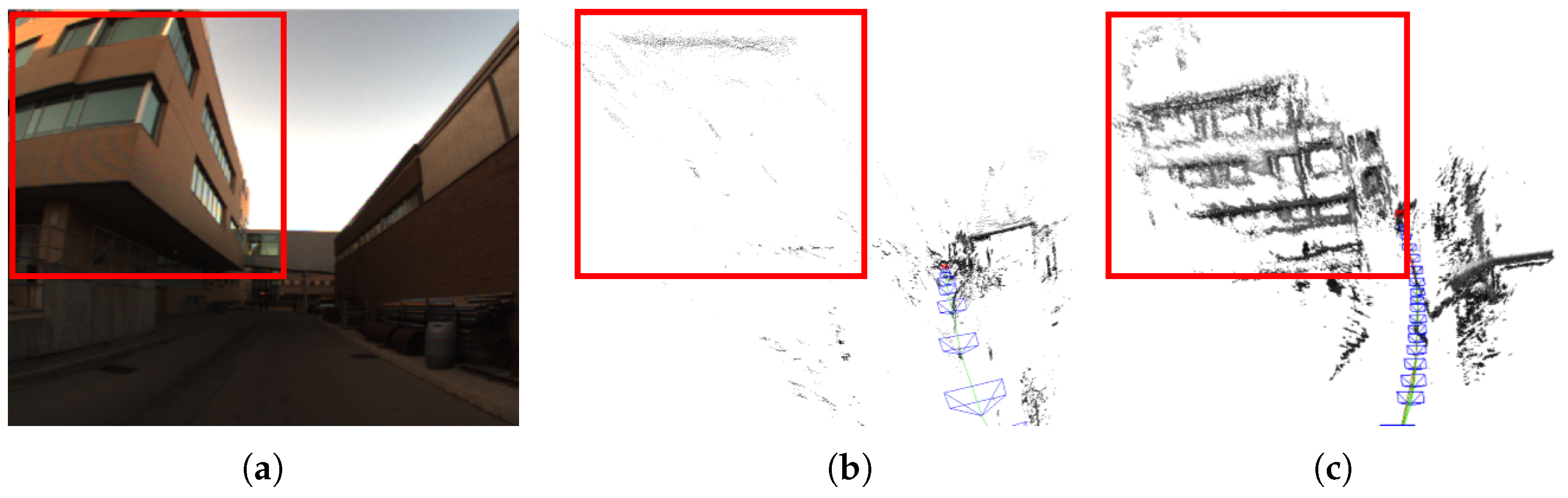
Since we did not have any way to estimate the ground truth pose accurately, the results shown here are only qualitative. We highlight a portion of the environment (a building) in the RGB image as seen in Figure 12a, the same region as reconstructed using tightly coupled approach in Figure 12b and using our method in Figure 12c. Notice the significant degradation in map quality due to tight coupling in presence of high inertial noise. As mapping is done in a SLAM framework, the error in pose prediction affects the quality of map that is built consequently. Since our approach is resilient to high inertial noise (as shown in an indoor settings, using quantitative results), the quality of the map built using our technique is superior.
8. Conclusions
In this work, a semi-tightly coupled direct visual-inertial fusion scheme was developed to handle sudden, unintended bumps encountered when the camera–IMU system is mounted on a land-vehicle. The multitude of visual correspondences provide enough constraints to correct large inter-frame IMU drifts. Further, by accounting for inverse-depth variances in our optimization framework, we can include information from all valid pixels in our inertial-epipolar optimization, making our fusion method a direct-approach. Although, an IMU has traditionally been used to speed up the prediction in a tightly-coupled framework, through experiments it was shown that a wrong prior at the start makes the joint optimization objective converge to a local minima. Hence, we found it reasonable to isolate the IMU measurements and correct it later by imposing epipolar constraints. We repeated the experiments for six different trajectories to confirm the validity of our approach. As a qualitative test, it was shown that the increased accuracy in pose estimation results in a consistent map, especially in the presence of sudden spikes. Since our approach uses two optimization objectives instead of one, it requires a minor computational overhead (~10 iterations, 12 ± 5 ms), while still achieving real-time speed. A trade-off in speed is the price paid to overcome inaccuracies due to bumps. Our technique is best suited for off-road land vehicles which are prone to sudden bumps and change of terrain. However, in cases where computational resource is limited and the noise due to motion can be appropriately modelled, the tightly-coupled approach can be used. In this paper, the drift in the poses and features were not considered, which can be investigated as future work. Also, augmentation of the the approach presented in this paper with loop-closure, relocalization and a pose-graph structure for long-term localization and mapping would be interesting to investigate as the next work.
Author Contributions
Conceptualization, M.B. and W.M.; methodology, B.S.; formal analysis, B.S.; resources, W.M.; data curation, B.S.; writing—original draft preparation, B.S.; writing—review and editing, M.B.; supervision, M.B. and W.M.; project administration, M.B. and W.M.; funding acquisition, W.M. and M.B. All authors have read and agreed to the published version of the manuscript.
Funding
This research was funded by NSERC Discovery Grant.
Institutional Review Board Statement
Not applicable.
Informed Consent Statement
Not applicable.
Data Availability Statement
Not applicable.
Acknowledgments
Financial support from the NSERC Discovery Grant is very much appreciated.
Conflicts of Interest
The authors declare no conflict of interest.
Appendix A
This appendix shows some of the trajectories:
Figure A1.
Trajectory #2: (a) Translation Errors (m) versus Image frame number (b) Angular Errors (rad) versus Image Frame number. Note: The coordinate frame expressed here is Camera centric: Z-forward, Y-down and X-right.
Figure A1.
Trajectory #2: (a) Translation Errors (m) versus Image frame number (b) Angular Errors (rad) versus Image Frame number. Note: The coordinate frame expressed here is Camera centric: Z-forward, Y-down and X-right.

Figure A2.
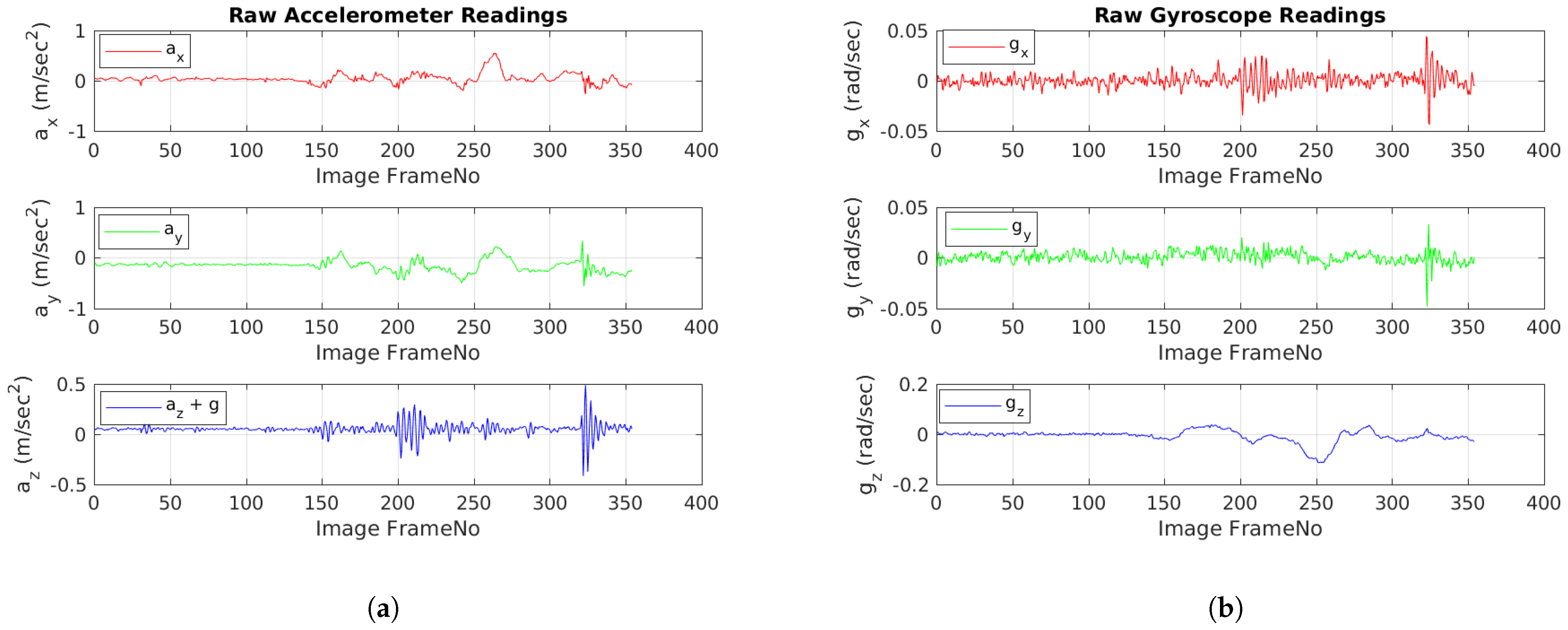
Trajectory #2: (a) Raw Accelerometer Reading versus IMU frame number. (b) Raw Gyroscope Reading versus IMU Frame Number. Note, that even though IMU sampling rate (100 Hz) is twice that of the camera (50 Hz), the readings are plotted with respect to Image Frame No. for easy comparison. Also note that the coordinate system in IMU centric: X-forward, Y-right, Z-down.
Figure A2.
Trajectory #2: (a) Raw Accelerometer Reading versus IMU frame number. (b) Raw Gyroscope Reading versus IMU Frame Number. Note, that even though IMU sampling rate (100 Hz) is twice that of the camera (50 Hz), the readings are plotted with respect to Image Frame No. for easy comparison. Also note that the coordinate system in IMU centric: X-forward, Y-right, Z-down.

Figure A3.
Trajectory #3: (a) Translation Errors (m) versus Image frame number (b) Angular Errors (rad) versus Image Frame number. Note: The coordinate frame expressed here is Camera centric: Z-forward, Y-down and X-right.
Figure A3.
Trajectory #3: (a) Translation Errors (m) versus Image frame number (b) Angular Errors (rad) versus Image Frame number. Note: The coordinate frame expressed here is Camera centric: Z-forward, Y-down and X-right.

Figure A4.
Trajectory #3: (a) Raw Accelerometer Reading versus IMU frame number. (b) Raw Gyroscope Reading versus IMU Frame Number. Note, that even though IMU sampling rate (100 Hz) is twice that of the camera (50 Hz), the readings are plotted with respect to Image Frame No. for easy comparison. Also note that the coordinate system in IMU centric: X-forward, Y-right, Z-down.

References
- Hu, H.; Sun, H.; Ye, P.; Jia, Q.; Gao, X. Multiple Maps for the Feature-based Monocular SLAM System. J. Intell. Robot. Syst. 2019, 94, 389–404. [Google Scholar] [CrossRef]
- Urzua, S.; Munguía, R.; Grau, A. Monocular SLAM System for MAVs Aided with Altitude and Range Measurements: A GPS-free Approach. J. Intell. Robot. Syst. 2019, 94, 203–217. [Google Scholar] [CrossRef] [Green Version]
- Nützi, G.; Weiss, S.; Scaramuzza, D.; Siegwart, R. Fusion of IMU and Vision for Absolute Scale Estimation in Monocular SLAM. J. Intell. Robot. Syst. 2011, 61, 287–299. [Google Scholar] [CrossRef] [Green Version]
- Steder, B.; Grisetti, G.; Stachniss, C.; Burgard, W. Visual SLAM for Flying Vehicles. IEEE Trans. Robot. 2008, 24, 1088–1093. [Google Scholar] [CrossRef] [Green Version]
- Zhou, F.; Duh, H.B.L.; Billinghurst, M. Trends in Augmented Reality Tracking, Interaction and Display: A Review of Ten Years of ISMAR. In Proceedings of the 7th IEEE/ACM International Symposium on Mixed and Augmented Reality, ISMAR ’08, Cambridge, UK, 15–18 September 2008; IEEE Computer Society: Washington, DC, USA, 2008; pp. 193–202. [Google Scholar] [CrossRef] [Green Version]
- Davison, A.J.; Reid, I.D.; Molton, N.D.; Stasse, O. MonoSLAM: Real-Time Single Camera SLAM. IEEE Trans. Pattern Anal. Mach. Intell. 2007, 29, 1052–1067. [Google Scholar] [CrossRef] [PubMed] [Green Version]
- Civera, J.; Davison, A.J.; Montiel, J.M.M. Inverse Depth Parametrization for Monocular SLAM. IEEE Trans. Robot. 2008, 24, 932–945. [Google Scholar] [CrossRef] [Green Version]
- Klein, G.; Murray, D. Parallel Tracking and Mapping for Small AR Workspaces. In Proceedings of the Sixth IEEE and ACM International Symposium on Mixed and Augmented Reality (ISMAR’07), Nara, Japan, 13–16 November 2007. [Google Scholar]
- Newcombe, R.A.; Lovegrove, S.J.; Davison, A.J. DTAM: Dense tracking and mapping in real-time. In Proceedings of the IEEE International Conference on Computer Vision, Barcelona, Spain, 6–13 November 2011; pp. 2320–2327. [Google Scholar]
- Newcombe, R.A.; Izadi, S.; Hilliges, O.; Molyneaux, D.; Kim, D.; Davison, A.J.; Kohi, P.; Shotton, J.; Hodges, S.; Fitzgibbon, A. KinectFusion: Real-time dense surface mapping and tracking. In Proceedings of the 2011 10th IEEE International Symposium on Mixed and Augmented Reality, Basel, Switzerland, 26–29 October 2011; pp. 127–136. [Google Scholar] [CrossRef] [Green Version]
- Whelan, T.; Salas-Moreno, R.F.; Glocker, B.; Davison, A.J.; Leutenegger, S. ElasticFusion: Real-time dense SLAM and light source estimation. Int. J. Robot. Res. 2016, 35, 1697–1716. [Google Scholar] [CrossRef] [Green Version]
- Whelan, T.; Kaess, M.; Johannsson, H.; Fallon, M.; Leonard, J.; McDonald, J. Real-time Large Scale Dense RGB-D SLAM with Volumetric Fusion. Intl. J. Robot. Res. 2014, 34, 598–626. [Google Scholar] [CrossRef] [Green Version]
- Bloesch, M.; Burri, M.; Omari, S.; Hutter, M.; Siegwart, R. Iterated extended Kalman filter based visual-inertial odometry using direct photometric feedback. Int. J. Robot. Res. 2017, 36, 1053–1072. [Google Scholar] [CrossRef] [Green Version]
- Mur-Artal, R.; Montiel, J.M.M.; Tardós, J.D. ORB-SLAM: A Versatile and Accurate Monocular SLAM System. IEEE Trans. Robot. 2015, 31, 1147–1163. [Google Scholar] [CrossRef] [Green Version]
- Mur-Artal, R.; Tardós, J.D. ORB-SLAM2: An Open-Source SLAM System for Monocular, Stereo and RGB-D Cameras. IEEE Trans. Robot. 2017, 33, 1255–1262. [Google Scholar] [CrossRef] [Green Version]
- Engel, J.; Sturm, J.; Cremers, D. Semi-Dense Visual Odometry for a Monocular Camera. In Proceedings of the IEEE International Conference on Computer Vision (ICCV), Sydney, Australia, 1–8 December 2013. [Google Scholar]
- Caruso, D.; Engel, J.; Cremers, D. Large-Scale Direct SLAM for Omnidirectional Cameras. In Proceedings of the International Conference on Intelligent Robots and Systems (IROS), Hamburg, Germany, 28 September–2 October 2015. [Google Scholar]
- Engel, J.; Stueckler, J.; Cremers, D. Large-Scale Direct SLAM with Stereo Cameras. In Proceedings of the International Conference on Intelligent Robots and Systems (IROS), Hamburg, Germany, 28 September–2 October 2015. [Google Scholar]
- Engel, J.; Schöps, T.; Cremers, D. LSD-SLAM: Large-Scale Direct Monocular SLAM. In Proceedings of the European Conference on Computer Vision (ECCV), Zurich, Switzerland, 6–12 September 2014. [Google Scholar]
- Kümmerle, R.; Grisetti, G.; Strasdat, H.; Konolige, K.; Burgard, W. g2o: A General Framework for Graph Optimization. In Proceedings of the 2011 IEEE International Conference on Robotics and Automation, Shanghai, China, 9–13 May 2011. [Google Scholar]
- Concha, A.; Civera, J. DPPTAM: Dense piecewise planar tracking and mapping from a monocular sequence. In Proceedings of the 2015 IEEE/RSJ International Conference on Intelligent Robots and Systems (IROS), Hamburg, Germany, 28 September–2 October 2015; pp. 5686–5693. [Google Scholar] [CrossRef] [Green Version]
- Concha, A.; Civera, J. Using superpixels in monocular SLAM. In Proceedings of the 2014 IEEE International Conference on Robotics and Automation (ICRA), Hong Kong, China, 31 May–7 June 2014; pp. 365–372. [Google Scholar] [CrossRef] [Green Version]
- Greene, W.N.; Ok, K.; Lommel, P.; Roy, N. Multi-level mapping: Real-time dense monocular SLAM. In Proceedings of the 2016 IEEE International Conference on Robotics and Automation (ICRA), Stockholm, Sweden, 16–21 May 2016; pp. 833–840. [Google Scholar] [CrossRef] [Green Version]
- Forster, C.; Zhang, Z.; Gassner, M.; Werlberger, M.; Scaramuzza, D. SVO: Semidirect Visual Odometry for Monocular and Multicamera Systems. IEEE Trans. Robot. 2017, 33, 249–265. [Google Scholar] [CrossRef] [Green Version]
- Mourikis, A.I.; Roumeliotis, S.I. A Multi-State Constraint Kalman Filter for Vision-aided Inertial Navigation. In Proceedings of the 2007 IEEE International Conference on Robotics and Automation, Roma, Italy, 10–14 April 2007; pp. 3565–3572. [Google Scholar] [CrossRef]
- Wu, K.; Ahmed, A.; Georgiou, G.; Roumeliotis, S. A Square Root Inverse Filter for Efficient Vision-aided Inertial Navigation on Mobile Devices. In Proceedings of the Robotics: Science and Systems, Rome, Italy, 13–17 July 2015. [Google Scholar]
- Qin, T.; Shen, S. Robust initialization of monocular visual-inertial estimation on aerial robots. In Proceedings of the 2017 IEEE/RSJ International Conference on Intelligent Robots and Systems (IROS), Vancouver, BC, Canada, 24–28 September 2017; pp. 4225–4232. [Google Scholar] [CrossRef]
- Forster, C.; Carlone, L.; Dellaert, F.; Scaramuzza, D. On-Manifold Preintegration for Real-Time Visual–Inertial Odometry. IEEE Trans. Robot. 2017, 33, 1–21. [Google Scholar] [CrossRef] [Green Version]
- Kschischang, F.R.; Frey, B.J.; Loeliger, H.A. Factor graphs and the sum-product algorithm. IEEE Trans. Inf. Theory 2001, 47, 498–519. [Google Scholar] [CrossRef] [Green Version]
- Concha, A.; Loianno, G.; Kumar, V.; Civera, J. Visual-inertial direct SLAM. In Proceedings of the 2016 IEEE International Conference on Robotics and Automation (ICRA), Stockholm, Sweden, 16–21 May 2016; pp. 1331–1338. [Google Scholar] [CrossRef]
- Bradler, H.; Ochs, M.; Fanani, N.; Mester, R. Joint Epipolar Tracking (JET): Simultaneous Optimization of Epipolar Geometry and Feature Correspondences. In Proceedings of the 2017 IEEE Winter Conference on Applications of Computer Vision (WACV), Santa Rosa, CA, USA, 24–31 March 2017; pp. 445–453. [Google Scholar] [CrossRef] [Green Version]
- Baker, S.; Matthews, I. Lucas-Kanade 20 Years On: A Unifying Framework. Int. J. Comput. Vis. 2004, 56, 221–255. [Google Scholar] [CrossRef]
- Huber, P.J. Robust Estimation of a Location Parameter. Ann. Math. Statist. 1964, 35, 73–101. [Google Scholar] [CrossRef]
- Furgale, P.; Rehder, J.; Siegwart, R. Unified temporal and spatial calibration for multi-sensor systems. In Proceedings of the 2013 IEEE/RSJ International Conference on Intelligent Robots and Systems, Tokyo, Japan, 3–7 November 2013; pp. 1280–1286. [Google Scholar] [CrossRef]
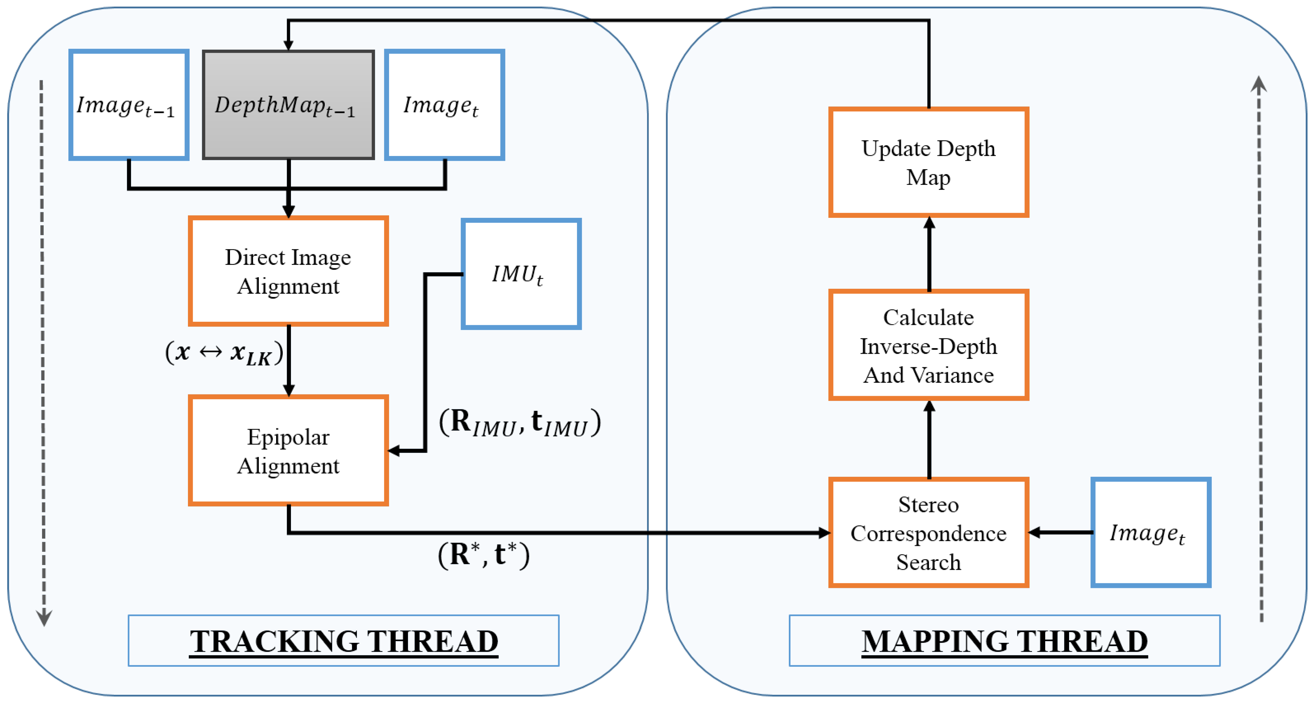
Figure 1.
Schematic for Visual Inertial Epipolar Constrained Odometry. Two threads run in parallel. The tracking thread encodes the epipolar optimization and the mapping thread uses the optimized pose () to update the map.
Figure 1.
Schematic for Visual Inertial Epipolar Constrained Odometry. Two threads run in parallel. The tracking thread encodes the epipolar optimization and the mapping thread uses the optimized pose () to update the map.

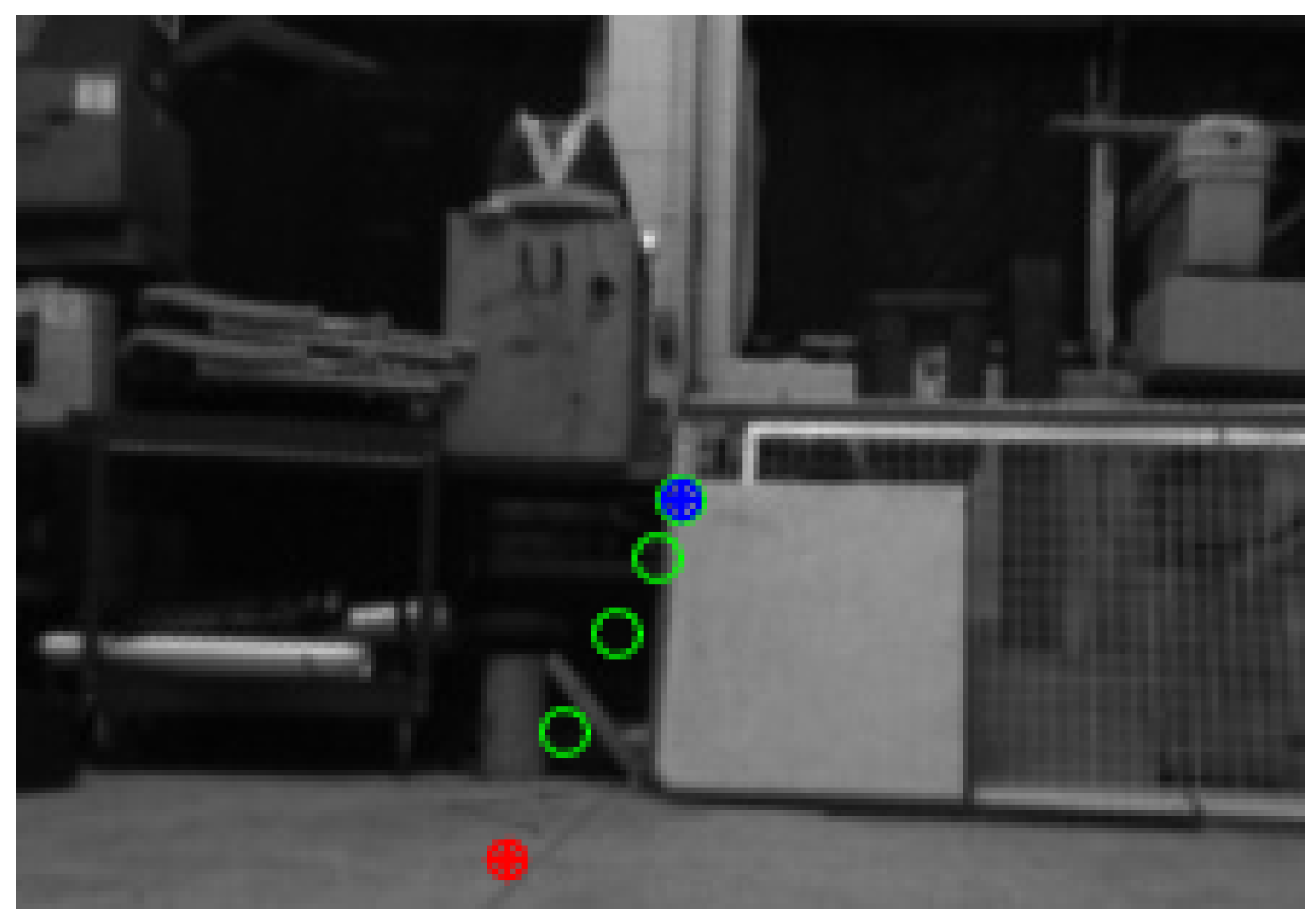
Figure 2.
The epipole positions plotted on the keyframe image during an optimization process for a straight line motion. RED shows the epipole position due to noisy prior due to integration of IMU measurements at the start of the optimization. GREEN shows intermediate epipole positions during the optimization. BLUE is the final epipole position. Since the trajectory is straight, the epipole’s image on the keyframe image should be at the centre of the image, which is where the initial noisy pose prior is driven to, as a result of optimization.

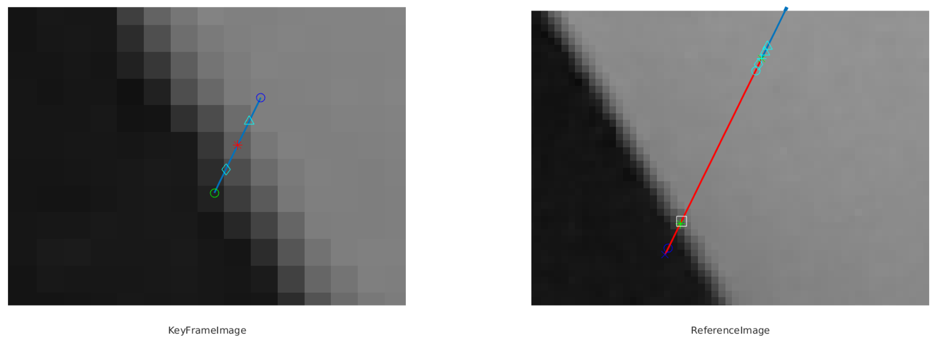
Figure 3.
Epipolar Stereo Matching on Keyframe and Reference Images. On the left are five equidistant points on the keyframe image and on the right, are the same five points being searched along the epipolar line (shown as RED line). The best match point, is shown as a box.
Figure 3.
Epipolar Stereo Matching on Keyframe and Reference Images. On the left are five equidistant points on the keyframe image and on the right, are the same five points being searched along the epipolar line (shown as RED line). The best match point, is shown as a box.

Figure 4.
SSD Error as five equidistant points are checked along the epipolar line (See Figure 3) in the reference image. The minima is the point of best match.
Figure 4.
SSD Error as five equidistant points are checked along the epipolar line (See Figure 3) in the reference image. The minima is the point of best match.

Figure 5.
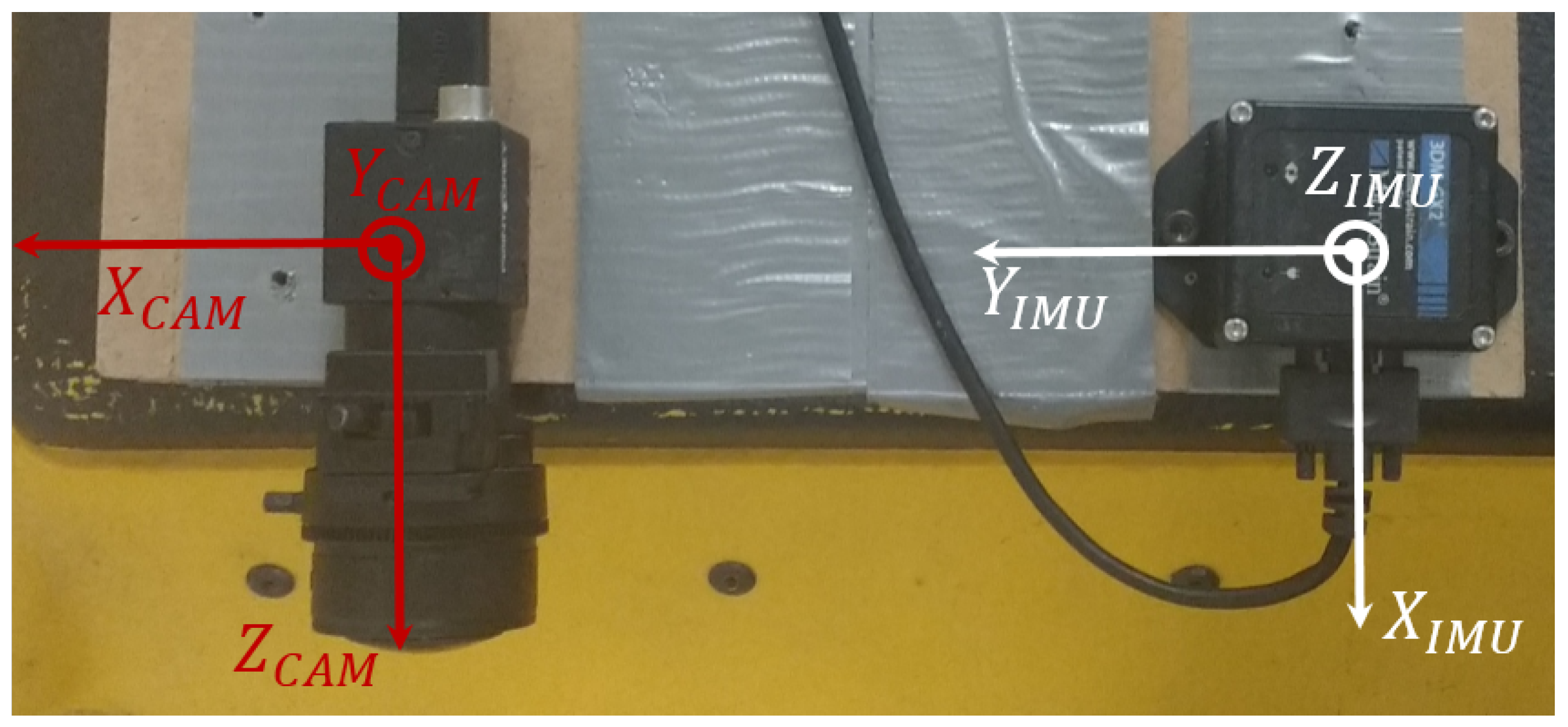
Camera–Inertial Measurement Unit (IMU) setup close-up view. Axis conventions shown for clarity.
Figure 5.
Camera–Inertial Measurement Unit (IMU) setup close-up view. Axis conventions shown for clarity.

Figure 6.
Indoor Experiment Setup. The monocular camera and IMU fixed rigidly and mounted on a trolley-cart with one misaligned wheel.
Figure 6.
Indoor Experiment Setup. The monocular camera and IMU fixed rigidly and mounted on a trolley-cart with one misaligned wheel.

Figure 7.
Outdoor Experiment Setup. The monocular camera and IMU fixed rigidly and mounted on an off-road vehicle. The axis conventions are shown in Figure 5.
Figure 7.
Outdoor Experiment Setup. The monocular camera and IMU fixed rigidly and mounted on an off-road vehicle. The axis conventions are shown in Figure 5.

Figure 8.
Temporal offset between Camera and IMU sampling.

Figure 9.
(a) Raw Accelerometer Reading versus IMU frame number. (b) Raw Gyroscope Reading versus IMU Frame Number. Note, that even though IMU sampling rate(100 Hz) is twice that of the camera (50 Hz), the readings are plotted with respect to Image Frame No. for easy comparison. Also note that the coordinate system in IMU centric: X-forward, Y-Right, Z-Down.

Figure 10.
Trajectory #1: (a) Translation Errors (m) versus Image frame number (b) Angular Errors (rad) versus Image Frame number. Note: The coordinate frame expressed here is Camera centric: Z-forward, Y-down, and X-right.
Figure 10.
Trajectory #1: (a) Translation Errors (m) versus Image frame number (b) Angular Errors (rad) versus Image Frame number. Note: The coordinate frame expressed here is Camera centric: Z-forward, Y-down, and X-right.

Figure 11.
A semi-dense map build of an indoor corridor.

Figure 12.
Outdoor Experiment. A portion of the 3D structure is highlighted in RED in all three figures for comparison. (a) shows the sample RGB image seen by the camera. (b) shows reconstruction quality for tightly-coupled system. (c) shows reconstruction quality for our method. Notice the improvement in map quality due to increased accuracy of pose estimation. Also note that in (a), radial distortion has not been removed to represent the actual, wide FOV sensor data received by the camera.


Table 1.
Calibration parameters for our experiment.
| PARAMETER: | VALUE |
|---|---|
| IMU Variances: | 0.01 (m/s2) and 0.005 (rad/s) |
| Temporal Offset: | 0.002 s (See Figure 8) |
| Accelerometer Biases: | , |
| , | |
| Gyroscope Biases: | , |
| , | |
| : | |
| Radial Distortion Coeff: | −0.04, −0.017, 0.033, |
Table 2.
Accuracy in terms of (RMSE) of Visual Inertial Direct Method (VID) and our method (VIE). The smaller error is bold-faced for clarity.
Table 2.
Accuracy in terms of (RMSE) of Visual Inertial Direct Method (VID) and our method (VIE). The smaller error is bold-faced for clarity.
| Trajectory ID | X RMSE (m) | Y RMSE (m) | Z RMSE (m) | Yaw RMSE (rad) | Pitch RMSE (rad) | Roll RMSE (rad) | ||||||
|---|---|---|---|---|---|---|---|---|---|---|---|---|
| VID | VIE | VID | VIE | VID | VIE | VID | VIE | VID | VIE | VID | VIE | |
| #1 | 0.0381 | 0.0312 | 0.0933 | 0.0530 | 0.0569 | 0.0588 | 0.0213 | 0.0038 | 0.0635 | 0.0136 | 0.0426 | 0.0348 |
| #2 | 0.0273 | 0.0237 | 0.0059 | 0.0323 | 0.1154 | 0.1159 | 0.2805 | 0.0020 | 0.0456 | 0.0181 | 0.0284 | 0.0025 |
| #3 | 0.0564 | 0.0866 | 0.1979 | 0.0857 | 0.1305 | 0.1124 | 0.3528 | 0.0131 | 0.0832 | 0.0253 | 0.0628 | 0.1066 |
| #4 | 0.0841 | 0.0367 | 0.0526 | 0.0335 | 0.0709 | 0.0988 | 0.7987 | 0.0013 | 0.0567 | 0.0225 | 0.0416 | 0.0200 |
| #5 | 0.0792 | 0.0331 | 0.1333 | 0.0670 | 0.0554 | 0.0512 | 0.0138 | 0.0112 | 0.0295 | 0.0149 | 0.0243 | 0.0667 |
| #6 | 0.0939 | 0.0411 | 0.0739 | 0.0376 | 0.1203 | 0.0756 | 0.3134 | 0.0037 | 0.0269 | 0.0321 | 0.0175 | 0.0265 |
Publisher’s Note: MDPI stays neutral with regard to jurisdictional claims in published maps and institutional affiliations. |
© 2021 by the authors. Licensee MDPI, Basel, Switzerland. This article is an open access article distributed under the terms and conditions of the Creative Commons Attribution (CC BY) license (http://creativecommons.org/licenses/by/4.0/).
Share and Cite
MDPI and ACS Style
Sahoo, B.; Biglarbegian, M.; Melek, W. Monocular Visual Inertial Direct SLAM with Robust Scale Estimation for Ground Robots/Vehicles. Robotics 2021, 10, 23. https://0-doi-org.brum.beds.ac.uk/10.3390/robotics10010023
AMA Style
Sahoo B, Biglarbegian M, Melek W. Monocular Visual Inertial Direct SLAM with Robust Scale Estimation for Ground Robots/Vehicles. Robotics. 2021; 10(1):23. https://0-doi-org.brum.beds.ac.uk/10.3390/robotics10010023
Chicago/Turabian StyleSahoo, Bismaya, Mohammad Biglarbegian, and William Melek. 2021. "Monocular Visual Inertial Direct SLAM with Robust Scale Estimation for Ground Robots/Vehicles" Robotics 10, no. 1: 23. https://0-doi-org.brum.beds.ac.uk/10.3390/robotics10010023
Note that from the first issue of 2016, this journal uses article numbers instead of page numbers. See further details here.