On Fast Jerk–, Acceleration– and Velocity–Restricted Motion Functions for Online Trajectory Generation


Department of Mechanical Engineering, Aalen University, D-73430 Aalen, Germany
Robotics 2021, 10(1), 25; https://0-doi-org.brum.beds.ac.uk/10.3390/robotics10010025
Submission received: 7 January 2021
/
Revised: 25 January 2021
/
Accepted: 26 January 2021
/
Published: 1 February 2021
(This article belongs to the Section Intelligent Robots and Mechatronics)
Abstract
:Finding fast motion functions to get from an initial state (distance, velocity, acceleration) to a final one has been of interest for decades. For a solution to be practically relevant, restrictions on jerk, acceleration and velocity have to be taken into account. Such solutions use optimization algorithms or try to directly construct a motion function allowing online trajectory generation. In this contribution, we follow the latter strategy and present an approach which first deals with the situation where initial and final accelerations are 0, and then relates the general case as much as possible to this situation. This leads to a classification with just four major cases. A continuity argument guarantees full coverage of all situations which is not the case or is not clear for other available algorithms. We present several examples that show the variety of different situations and, thus, the complexity of the task. We also describe an implementation in MATLAB® and results from a huge number of test runs regarding accuracy and efficiency, thus demonstrating that the algorithm is suitable for online trajectory generation.
1. Introduction
For achieving high throughput in handling machines, one of the most basic tasks consists of quickly moving from one position to the next one, taking into account machine restrictions regarding velocity, acceleration and jerk. This task is generally known as “path and trajectory planning” for robots and other automatic machines [1,2], and beside short execution times, other goals such as low energy consumption or low jerk have been considered in [3]. In this contribution, we restrict ourselves to a one-dimensional case where a certain distance Δs is given and a motion function s(t) is to be found, such that symmetric restrictions regarding velocity v(t), acceleration a(t) and jerk j(t) apply, i.e., , and .
The limit to the jerk function implicitly requires the acceleration function to be continuous, whereas the jerk function is allowed to have discontinuities. This task can be sub-divided into subtasks regarding the given initial and final states (velocity and acceleration). In the classification given in the respective guideline of the German Association of Engineers [4], 16 combinations are stated depending on whether the initial state is (called “rest”: R), (G), (U) or (B) (German abbreviations). The most well-known task is RR (“rest-to-rest”), which, in robotics, is usually called “point-to-point motion”. Kröger and Wahl [5] provide a different classification that also includes the types of restrictions, but for our purposes, the VDI classification suffices.
The task of finding a fast (sometimes also called “optimal”) motion function has been investigated for several decades. Roughly, one can distinguish between two kinds of approaches: In the first approach, the task is formulated as a restricted optimization problem and then well-known or self-developed algorithms from the fields of parameter optimization or optimal control are used [6,7,8,9,10]. The class of functions considered are often spline functions [6,7,10]. Lin et al. [8] use a specific class of piecewise-defined functions (“seven segments”) which are optimized. Such approaches have the advantage that optimization can take into account further aspects by modifying the objective (goal) function, e.g., energy consumption or deviation from a certain path, and they can also handle variable restrictions on velocity, acceleration and jerk. On the other hand, they are more time-consuming, such that they are mainly used for so-called off-line trajectory construction taking place in advance as opposed to on-line trajectory planning where the trajectory is changed “on the fly” during a controller cycle due to unforeseen events [11,12].
The second approach constructs the motion function directly using piecewise-defined functions [1,13,14,15,16,17,18,19,20,21,22]. We first consider the most basic task, RR. Choosing a piecewise constant jerk function leads to the so-called seven-segment profile (depicted in Figure 1) with continuous acceleration but discontinuous jerk, which has been fully specified in [1] (pp. 90–93) and can be found in industrial implementations [13] (Section 11.2). The approach has been extended to a 15-segment profile with piecewise constant snap in [1] (pp. 107–114), making the jerk function continuous. Considerable improvements have been achieved by using higher-order polynomials or the sigmoid function [14,15]. They provide fast motion functions with continuity in higher-order derivatives (or even all derivatives [15]) and are, hence, very suitable for vibration reduction. Smoothing can also be achieved by applying moving averages, as is shown in [16]. It is open whether and how the use of such advanced functions can be extended to motion tasks other than RR. When non-zero values are prescribed for initial and/or final velocities and/or acceleration, direct construction seems to be much harder. Nearly all contributions known to the author use the relatively simple seven-segment profile since this already leads to complex computations. The subtask GG (zero acceleration at initial and final states) has been dealt with for seven-segment profiles by [17] and [1], but both solutions are incomplete (for [17], cf. Kröger [10] (Section 4.1.2)) or can be improved (in [1], absolute values of the occurring minimal and maximal acceleration are assumed to be equal even if they are lower than the limit value, cf. Example 3.11, p. 84). Using, also, the seven-segment profile, Haschke et al. [18] developed an algorithm for the subtask BR (arbitrary initial state, rest), and Kröger and Wahl [5] and Kröger [12] provided a solution for the subtask BG, going through all possible branches in their decision tree. Their work shows the complexity of the task since they could provide only a small portion of their decision trees in their publications (cf. [5] (p. 106) for information on the number of nodes in these trees).
For the general task BB (arbitrary values for initial and final velocities and accelerations), Ezair et al. [19] developed a recursive algorithm which even enables them to handle a case where initial and final values as well as restrictions are given for an arbitrary number of derivatives and higher orders of continuity can be achieved, but only for order 2 (i.e., continuous acceleration); the algorithm is fast enough for online trajectory generation. In this case, it provides a seven-segment profile but not necessarily the fastest one. As we will show, there might be several seven-segment profiles solving the problem with quite different execution times. Broquère [20] and Broquère et al. [21] present a complex algorithm for the seven-segment profile but, as observed by Kröger [12] (Section 4.1.2), their work does not provide a solution in all cases, and we will give examples in Section 4 for configurations which are easily overseen. Recently, Sidobre and Desormeaux [22] modified the work in [20,21] and developed an algorithm where they claim to be able to reduce the general situation to just four simple sub-cases, but there is no proof, and the claim is not supported by extensive test runs with random values for all input data.
It is the goal of this contribution to provide an algorithm for constructing a seven-segment profile for the general BB task which provenly covers all possible situations, has a clear systematic structure with manageable complexity and is efficient enough for being suitable for online trajectory generation. Note that our results have some overlap with those of Sidobre and Desormeaux [22], but we apply a different approach by reducing the general BB task as much as possible to the GG subtask using intermediate velocities. We do not claim to provide an optimal solution (although this might be the case) since we do not have mathematical proof for this. Therefore, we just label our solution as “fast” since, at any time, at least one restriction is exactly fulfilled, but we also show that this does not imply global optimality.
The paper is structured as follows: In the next section, we present the seven-segment motion profile with modifications and recall the “acceleration–velocity plane” introduced by Broquère et al. [20] and Broquère [21]. Section 3 models the subtask GG where initial and final velocities are 0 and, based on this, Section 4 deals with the general task. Section 5 discusses implementation issues and describes the results of the validation in MATLAB®. Section 6 summarizes the results and discusses further work.
2. Basic Models, Quantities and Visualizations
The task we want to solve in this contribution consists of finding a fast motion function when the following eight values are given:
, , (each > 0), such that , and ; initial conditions: , ; end conditions: , ; distance: Δs (arbitrary real numbers).
Note that the distance is meant to be the difference between the final and the initial value of the path scale (), not the “travelled distance”, which might be much longer when the motion goes back first and then forward again.
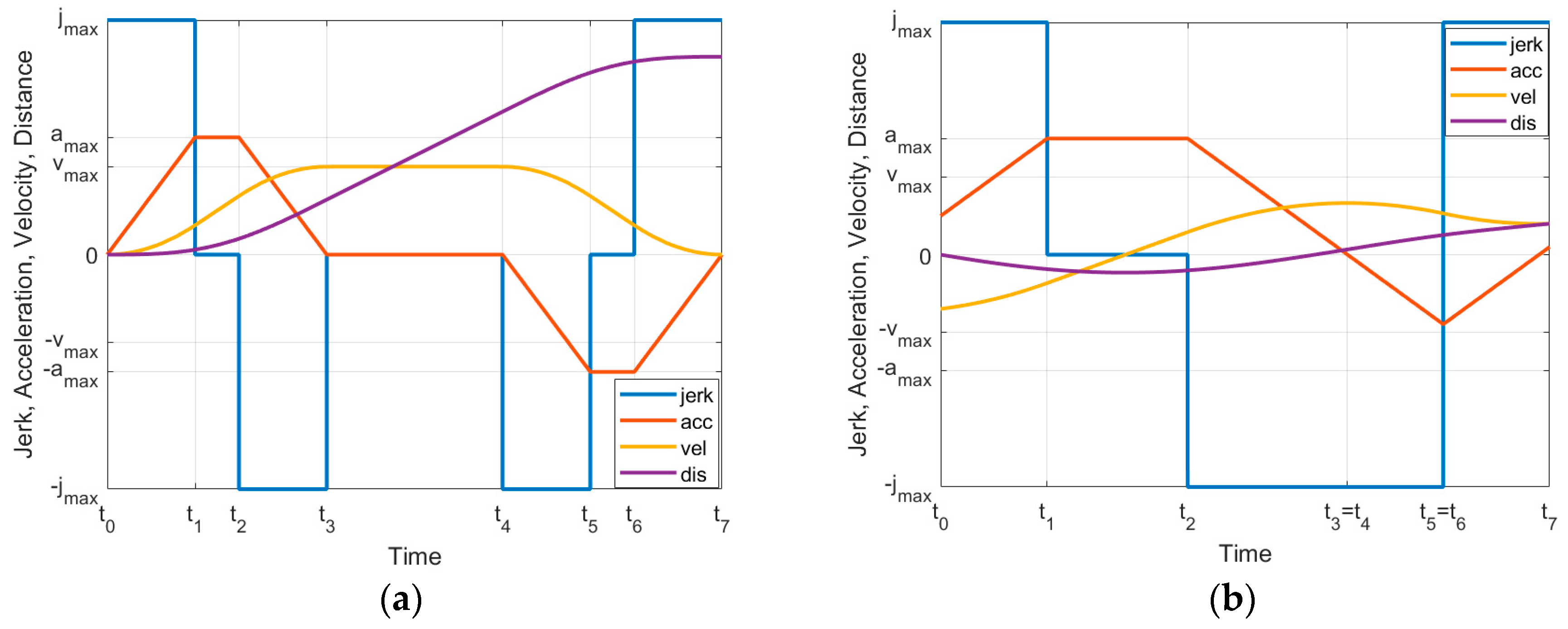
As in [20,21,22], we work with a so-called 7-segment motion profile, shown in Figure 1. It is based on a piecewise constant jerk function together with initial conditions on velocity and acceleration. In this profile, the motion function has, at most, 4 segments where the jerk is and, at most, 3 segments with zero jerk. In the classical RR situation (“rest-to-rest”, see Figure 1a), the sign pattern of the jerk segments is , but we allow arbitrary patterns such as to occur in order to have full coverage of all possible configurations as will be seen later. Formally stated, we have:
Note that all of these intervals might have zero length. In the example displayed in Figure 1a, the maximal values for velocity and acceleration are reached, which need not always be the case. Figure 1b provides an example for the general situation where , , and are non-zero. In that example, only is reached and two of the potentially seven segments have length zero.
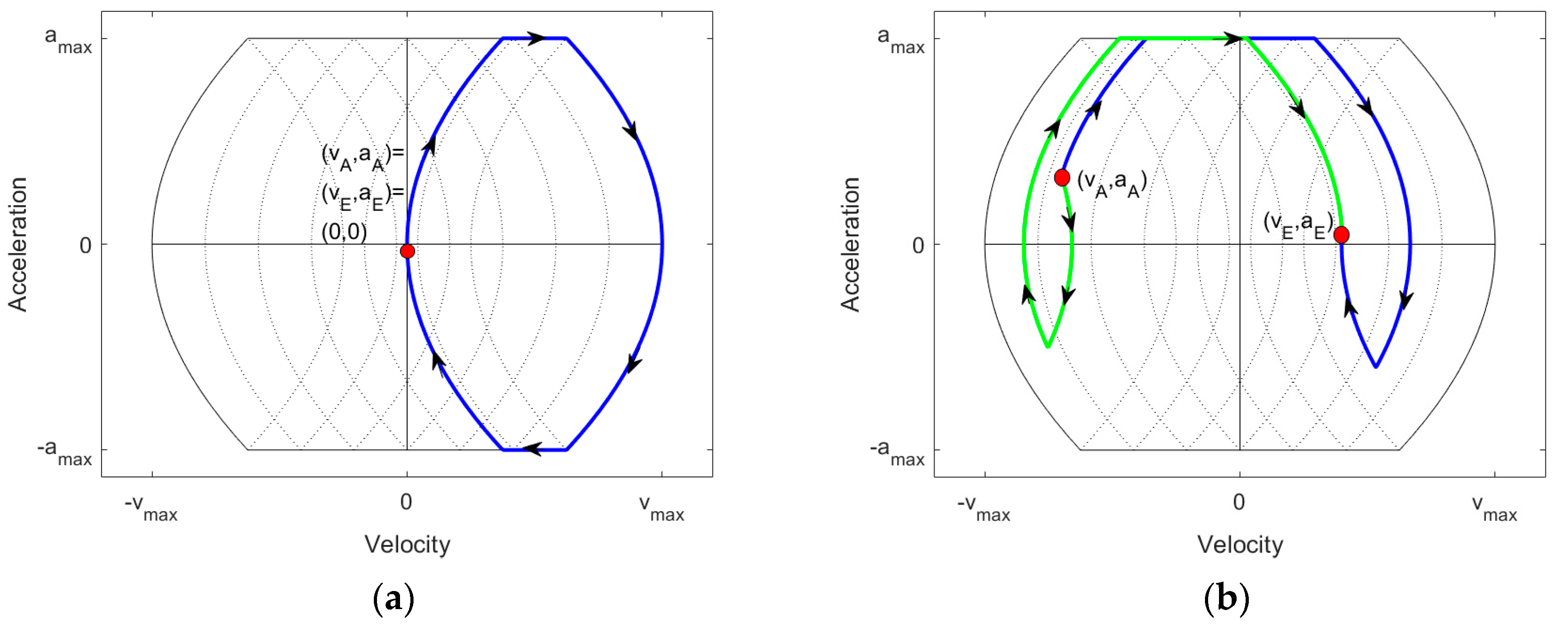
In order to visualize the change of velocity and acceleration in such seven-segment motion functions, Broquère [20,21] introduced the velocity–acceleration plane, shown in Figure 2. In this plane, motion functions are displayed mathematically as parametric curves . When one assumes that or 0, then the curves “move” along square root curves or horizontally (e.g., from and one obtains ). The square root curves can be of the kind (open to the right) or (open to the left) with constants . We assume that the horizontal motion only occurs when since otherwise, faster motion is possible. Motion along the square root curves is only possible clockwise since when the acceleration is positive (resp. negative), the velocity must increase (resp. decrease). The only points where a fast motion function might stay for a time of length >0 are the points (,0). This is the case when there is a segment with zero jerk and acceleration. Figure 2a shows a representation of the classical RR situation where and are reached. Note that only points within the area bounded by the left and right square root curves and the horizontal lines at and are admissible since only those points can be reached from (0,0) and one can go back from there to (0,0) without violating the restrictions (a larger opening of the square root curve corresponds to a higher value of ). The velocity–acceleration plane has one particular “pitfall” where misunderstandings can easily occur, so special care is called for: It does not show the distance ∆s, and this distance heavily depends on where in the velocity–acceleration plane a curve is placed. The length of the curve has nothing to do with the distance ∆s. The blue curve in Figure 2b depicts the motion function of Figure 1b (with positive ∆s) in the velocity–acceleration plane. The green curve has the same initial and end conditions but a negative value for ∆s.
3. The Subtask GG: Zero Acceleration Initially and Finally
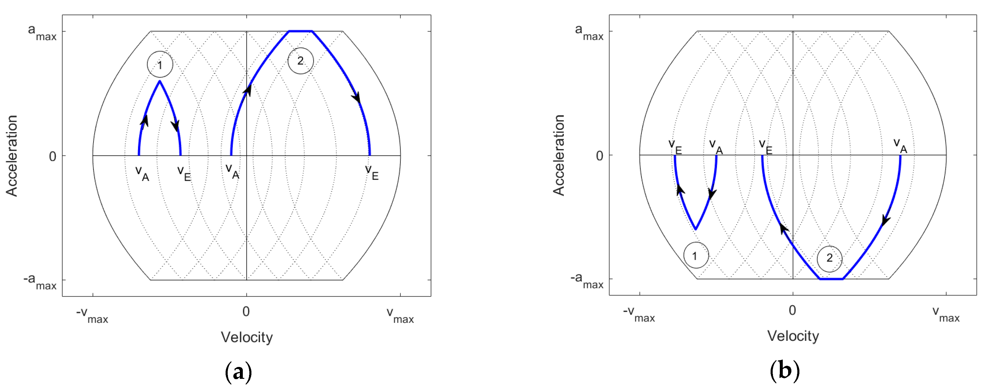
In this section, we consider a motion with zero acceleration initially and finally. Let resp. be the initial resp. final velocity. We first determine the time necessary to get from the initial to the final state by applying first maximal (minimal) jerk and then minimal (maximal) jerk where in between the jerk might be zero and the acceleration equal to . Examples are shown in Figure 3 in the velocity–acceleration plane. Type 1 depicts the situation where is so small that maximal/minimal acceleration is not reached, whereas in type 2, the latter is the case. When is just reached, we have , so type 1 occurs when and type 2 when .
In type 1, the maximally reached acceleration is , where T is the overall time. Hence, , and thus, . The distance travelled in this case is . In type 2, we have , and hence, . The distance travelled in this case is again . We summarize the result as follows:
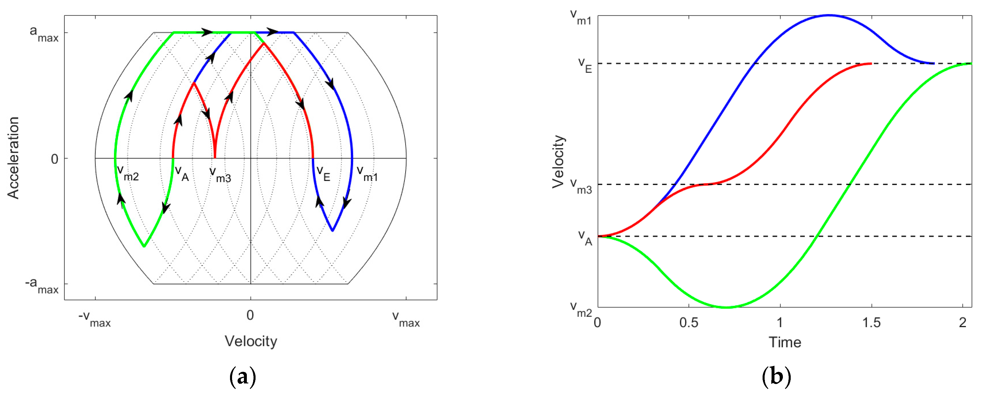
Figure 3 shows examples for the GG situation, each of which works just for one specific given distance. For other distances, the curve goes from to an intermediate velocity and then further on to the final velocity , as is shown in Figure 4 for three situations (, , ), where the third situation is not the fastest as we will see.
From (1) and (2), we can easily compute the overall time and distance when going via an intermediate velocity :
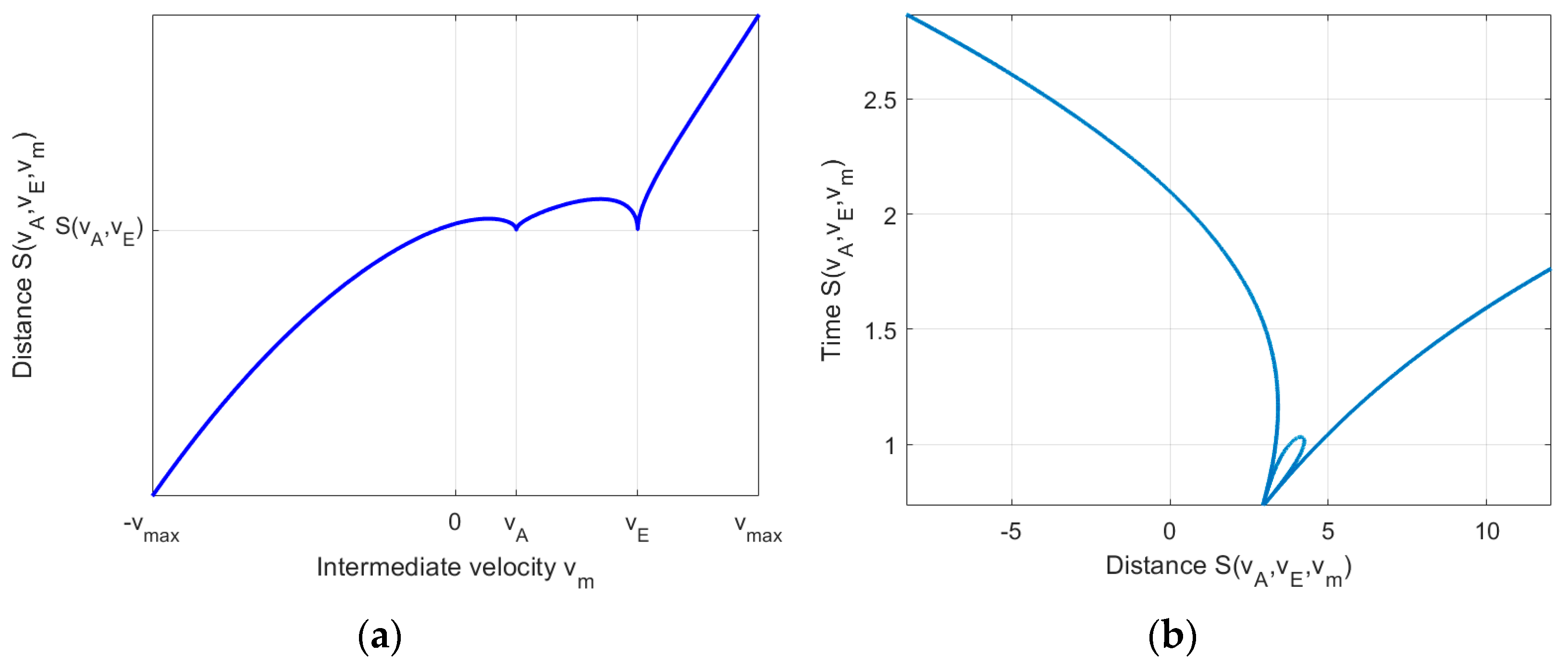
In order to visualize how the distance changes when and are fixed and runs from to , one can plot over , as shown in Figure 5a. For seeing in one plot how varies simultaneously, a parametric curve is adequate, as shown in Figure 5b. Both parts provide interesting information which will also be of use for the general situation (Section 4). If (resp. ) and remains constant for a certain time interval, the distance increases (resp. decreases) linearly with time. Therefore, in Figure 5b, the graph could be extended linearly to the left and to the right. We further observe that the distance varies continuously with , which follows mathematically from (2) and (3); therefore, for any given distance, a solution can be found.
The behavior shown in Figure 5a might be astonishing at first sight; the distance increases first when is below before decreasing monotonously. We explain this using Figure 4b. Here, there are two controversial effects: decreasing makes the velocity curve lie “lower”, leading to a smaller integral (less distance); on the other hand, the time needed to get to becomes larger, leading to a longer integration interval (larger distance). Obviously, in the long run, the first effect becomes dominant, but in the short term, the second one is dominant, leading to an increase in distance. This gives, already, an impression of the complexity of the situation, which is easily overlooked, leading to false assumptions.
Figure 5a shows that depending on the given distance, there are up to five solutions to the motion problem using an intermediate velocity . Five solutions occur when the given distance is slightly above . This also shows that the fact that, at any time, one of the restrictions is taken does not guarantee optimality. Figure 5b shows which solution is the fastest one; for a given distance, the lowest intersection of the vertical line at that distance with the curve provides the best solution. One can also observe that the best time is discontinuous over the given distance. In [22], Sidobre and Desormeaux also provide examples for this phenomenon. They also use a parametric curve of distance over time needed, but they use a different parameter (time).
For finding the best solution within the class of seven-segment functions, one has to solve the equation . We will explain how to do this efficiently in Section 5.
4. The General Task: Arbitrary Velocity and Acceleration, Initially and Finally
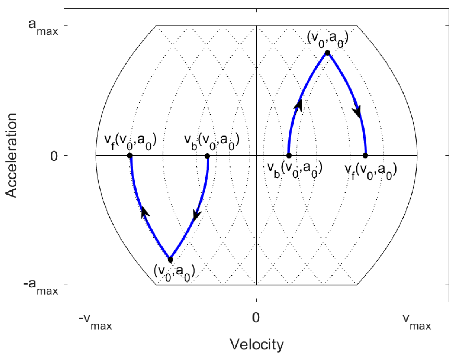
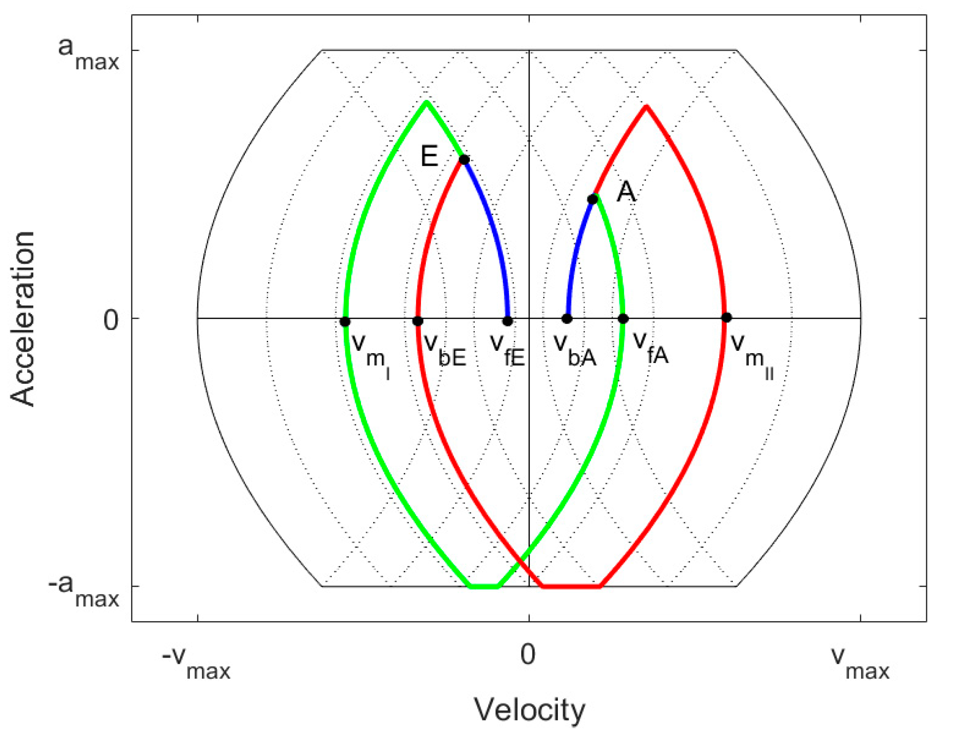
In this section, we consider the general case where initial and final velocities and accelerations can be arbitrary. We start with introducing some auxiliary functions that will be helpful in the later exposition. For an arbitrary admissible point in the velocity–acceleration plane, is defined to be the velocity for which the following holds: If you start at the point and apply minimum (resp. maximum) jerk if (resp. ), then you reach . The index b here stands for “backward”, i.e., going backward from . Figure 6 illustrates the definitions. Analogously, is defined to be the velocity for which the following holds: If you start at the point and apply maximum (resp. minimum) jerk if (resp. ), then you reach . The index f here stands for “forward”. An easy computation yields:
Moreover, let be the additional distance when one goes from to , applying minimum (resp. maximum) jerk if (resp. ). Analogously, is defined to be the distance when one goes from to , applying maximum (resp. minimum) jerk if (resp. ). Again, an easy computation shows:
Finally, let be the time needed to go from a point ( arbitrary) to (or, equivalently, to go from to ), applying maximum resp. minimum jerk. We have:
If one changes the positive direction of the distance, then the original problem is transformed into a problem with data −Δs, , , and which has the same solution regarding time intervals, only the sign factors for have to be changed (see Broquère, 2011). Therefore, we can restrict ourselves to two main situations: and , or and . The other combinations can be transformed into the former ones by changing the positive direction of distance. These two main cases are further split up into four sub-cases which depend additionally on , , and ; see Table 1.
From Table 1, it is logically clear that this is a complete coverage of all cases. We will see that only in case C do we need a further division into two sub-cases. In the sequel, we use the following abbreviations:
- ;
- ,, , ;
- ,, , ;
- , .
Our general procedure in the following treatment of the cases is based on the principle that we try to relate the general case BB as much as possible to the special case GG by either embedding the general case in a GG situation or extending a GG situation to the general case BB. We discuss case A in detail, elaborating on the lines of argumentation, and will then treat cases B–D shorter.
- Case A: and ,
In this case, E lies “right of” A in the sense that E lies on a square root curve (open to the right) right of the square root curve (open to the right) on which the point A lies or the curves are identical.
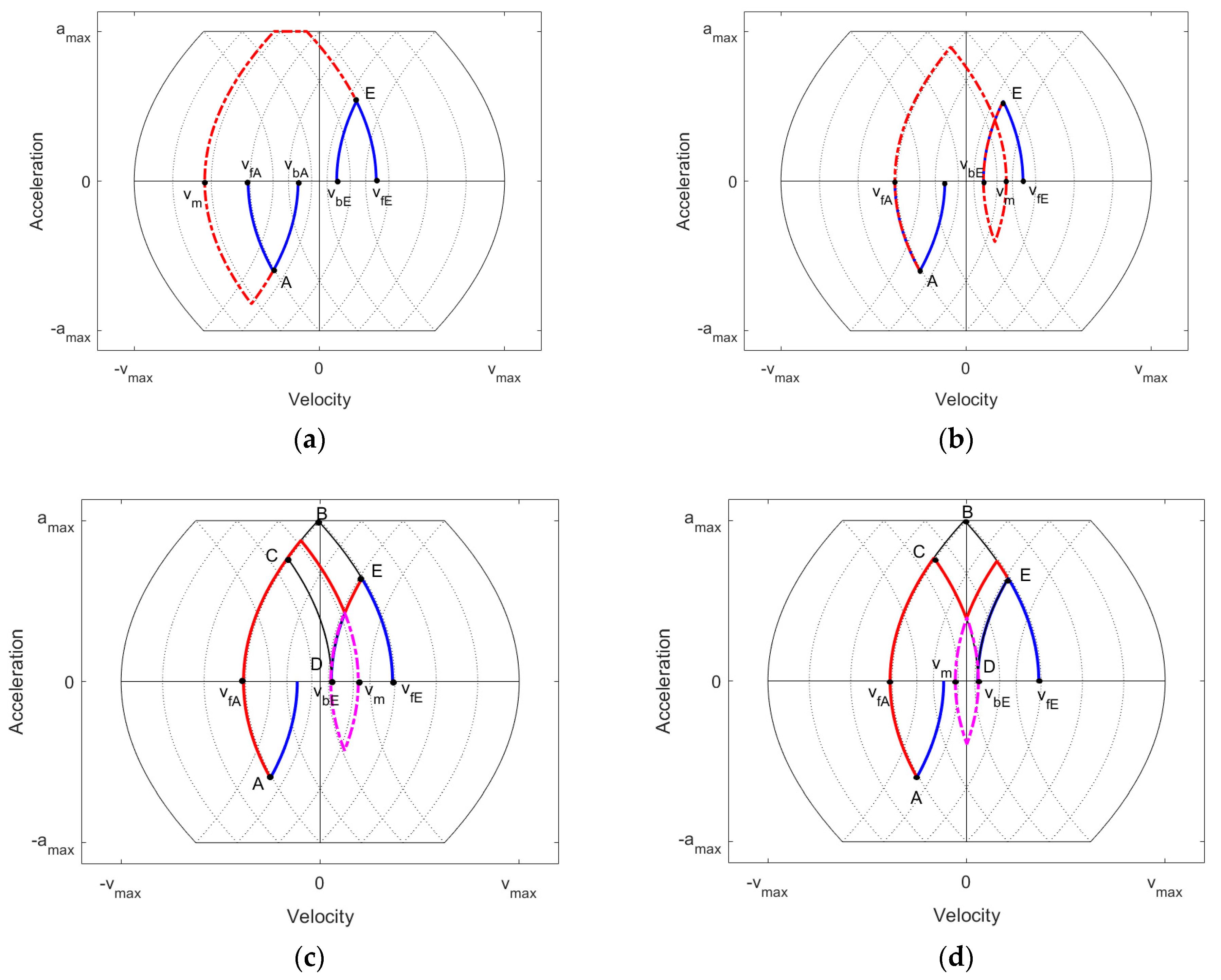
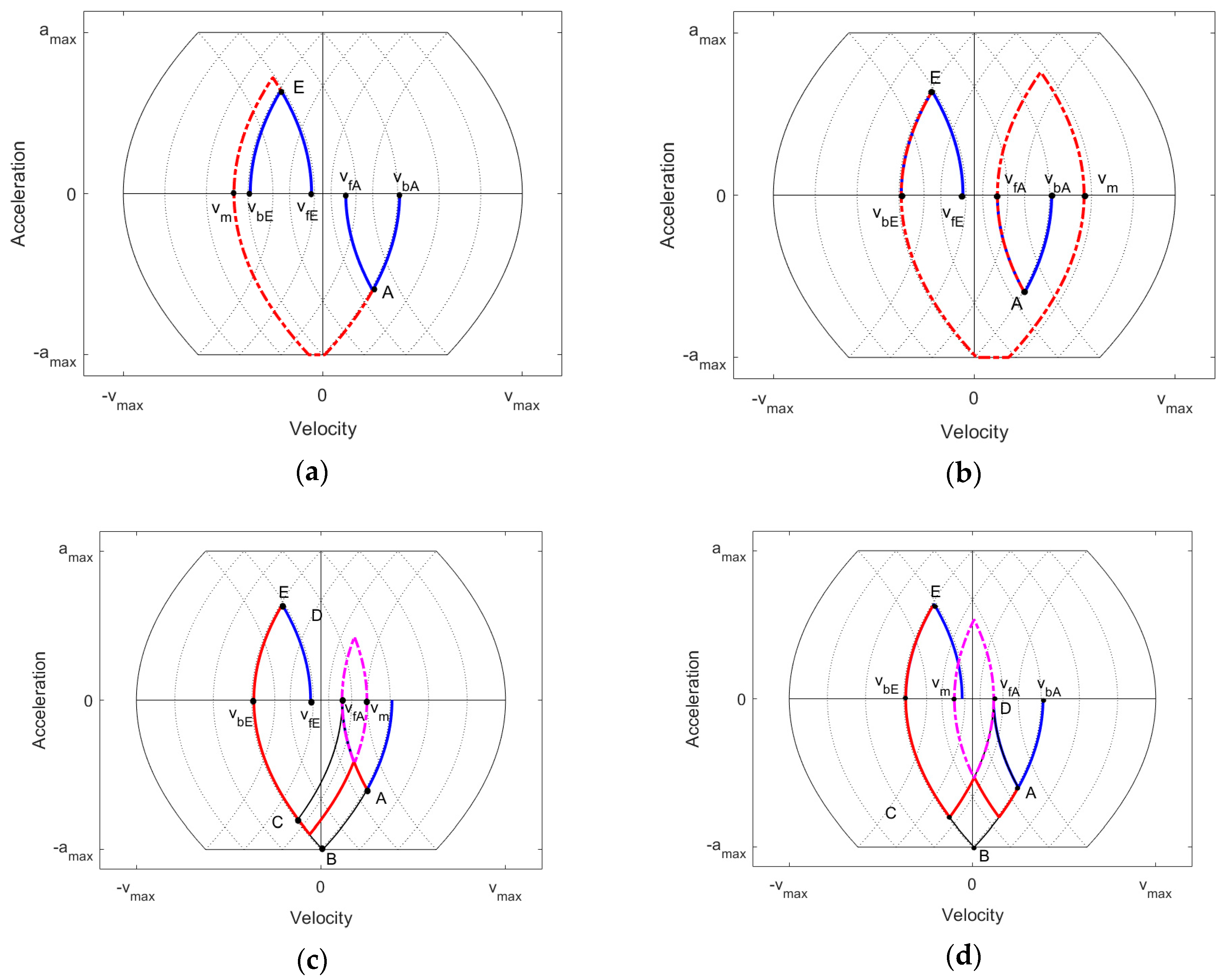
For a certain subset of all distances Δs, we can embed the task in a GG task for going from to via a as is shown in Figure 7a. Making smaller and inserting a phase with constant velocity enables us to realize arbitrarily small values for Δs (mathematically spoken: Δs goes to when the length of the phase with constant goes to ). We get the corresponding distances by computing:
Note that this holds for , but we will disregard, first, this restriction on and allow to be arbitrarily small and correct that later.
We can similarly cover arbitrarily large distances by extending the GG task going from to via a , as is shown in Figure 7b. When reaches , one can insert a phase with constant velocity . Again, we will disregard this restriction on first and correct that later. We obtain the corresponding distances by computing:
As we will see in examples, there might be a gap between the interval of distances covered in Part I and that covered in Part III. Distances in this gap can be achieved in two ways.
We again extend the GG task going from to via a with , where we let run from right to left (!), i.e., from to , and then “cut off” the part going from to and back to (shown in Figure 7c as a dashed pink curve). This continuously connects the distance covered in Part I when using with the distance covered in Part III when using . Therefore, we have a full coverage of all possible real distances. We obtain the corresponding distances by computing:
Another way to close the gap is a bit more complicated and is shown in Figure 7d. The first part up to point C is the same as in Part IIa, but then we have the sequence , , instead of , , in Part IIa. We can embed part of the curve in a GG task going from to via a with , as is shown in Figure 7d. Actually, can be replaced by since at , the minimal acceleration is reached and going on to the left with does not further change the distance Δs since the parts added are cut off again later, as can be seen by drawing a figure which is omitted here. We can compute the corresponding distances in the following way:
In our experiments (see the examples below), we have encountered a situation where a solution using Part IIb provides a shorter time than a solution using Part IIa, but then the distances were already covered by Part I or III, which provided even shorter times. However, since we have no mathematical proof that this is always the case, we simply include both possibilities. As we will see in the implementation section, this adds only the effort of finding the roots of three additional polynomials. Note that in case of or , parts IIa/b do not occur.
For each of the parts, the times needed can be easily computed:
As in the GG task, we can illustrate different situations by plotting as a parametric curve for parts I–III. We present a few examples showing interesting situations and behavior. In the examples, all distances have the unit m, velocities m/s, acceleration m/s2 and jerk m/s3. Units are omitted for the sake of brevity. As restrictions, we have chosen values similar as the ones used in [1]: , , .
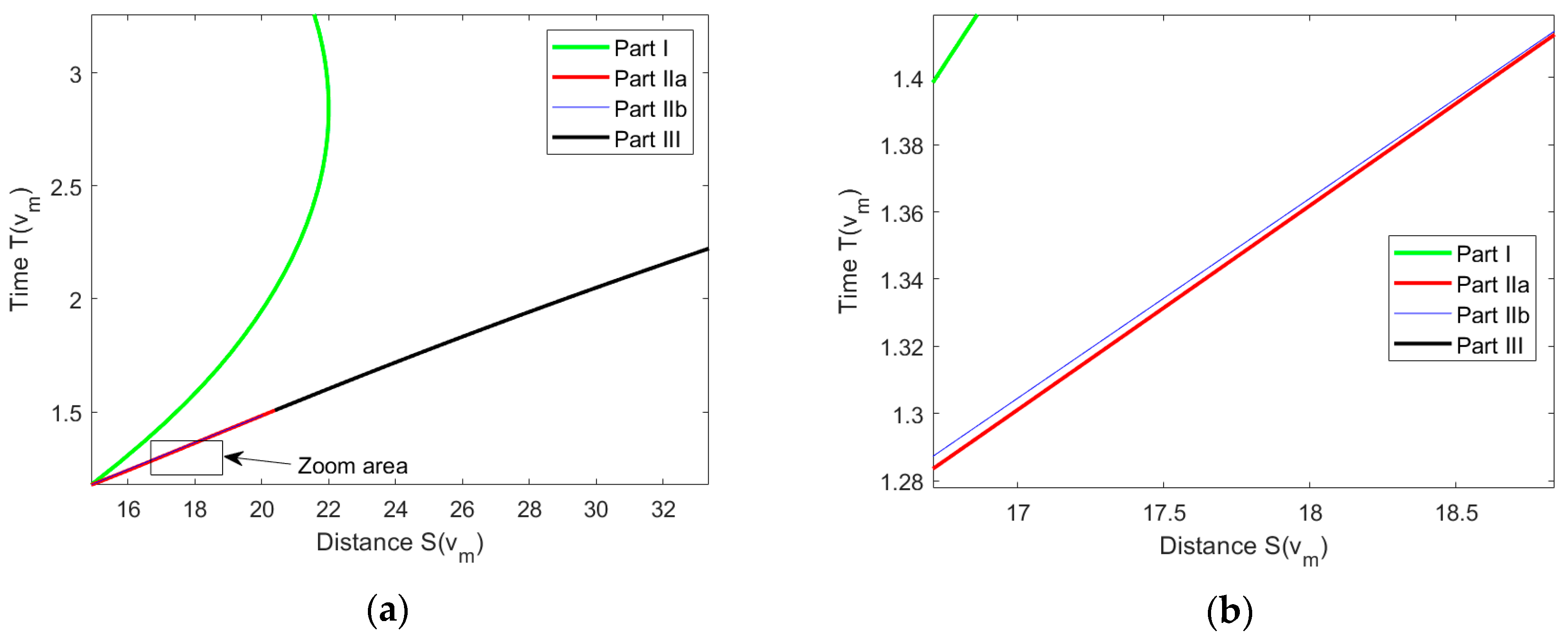
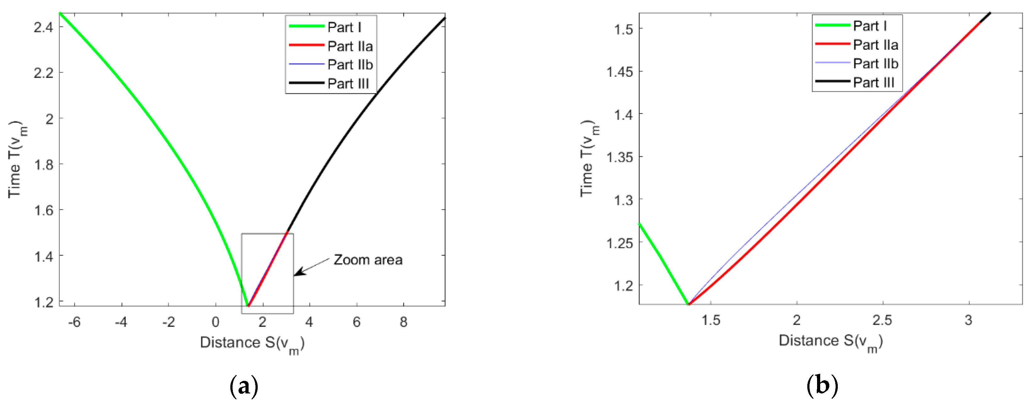
Example 1: No gap between Parts I and III, but Parts IIa or IIb are better.
Initial and final conditions: . Note that the colors used in the following figures have nothing to do with the colors used in Figure 7. The corresponding curve is shown in Figure 8a, where the green part (Part I) goes on to the left, covering arbitrarily small (negative) distances, and the black part (Part III) goes on to the right, covering arbitrarily large distances. One can see that Parts I and III cover all distances but Parts IIa and IIb provide solutions needing less time in the interval of distances where they are valid. There is no huge difference between Parts IIa and IIb, but when zooming in (Figure 8b), one can see that, in this example, the red part (Part IIa) is better. Figure 8 also shows that for a given distance, there might be several solutions in different parts or in the same part, as we have already recognized in the GG situation in Section 3. For example, for the distance Δs = 18, there are two solutions in Part I and one solution each in Parts IIa and IIb.
Example 2: No gap between Parts I and III, Parts IIa and IIb are not needed.
Initial and final conditions: . We use the same accelerations as in Example 1 but shift the velocities to the left by 28. In this way, variations are also produced in [22].
The corresponding curve is shown in Figure 9a. Again, the green part (Part I) goes on to the left, covering arbitrarily small (negative) distances, and the black part (Part III) goes on to the right, covering arbitrarily large distances. Parts I and III cover all distances and one of them provides the best solution, so Parts IIa and IIb are not needed. There is no huge difference between Parts IIa and IIb, but when zooming in (Figure 9b), one can see that, in this example, the blue part (Part IIb) is better. Part IIb provides a solution where the jerk changes sign three times (see Figure 7d), whereas in the solution of Part IIa, the jerk changes sign only two times. Therefore, the conjecture that solutions with less changes are better, which might look plausible at first sight, is wrong. What might be true is that the best solution (here from Part I) always has the lowest number of sign changes, but we do not have mathematical proof for this conjecture.
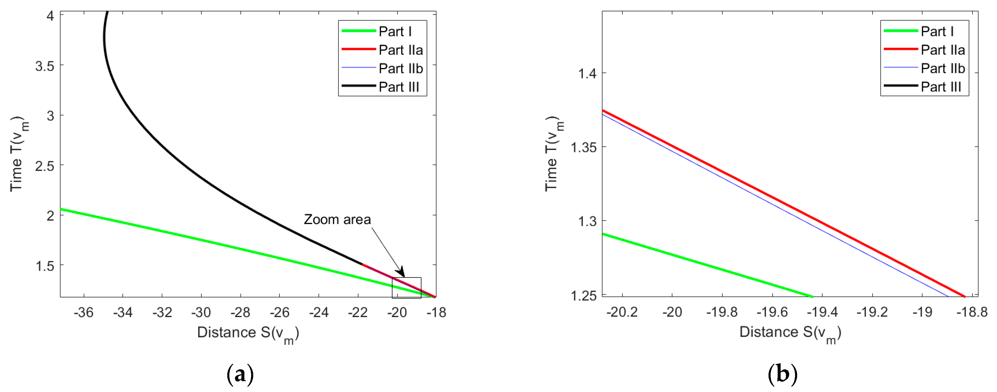
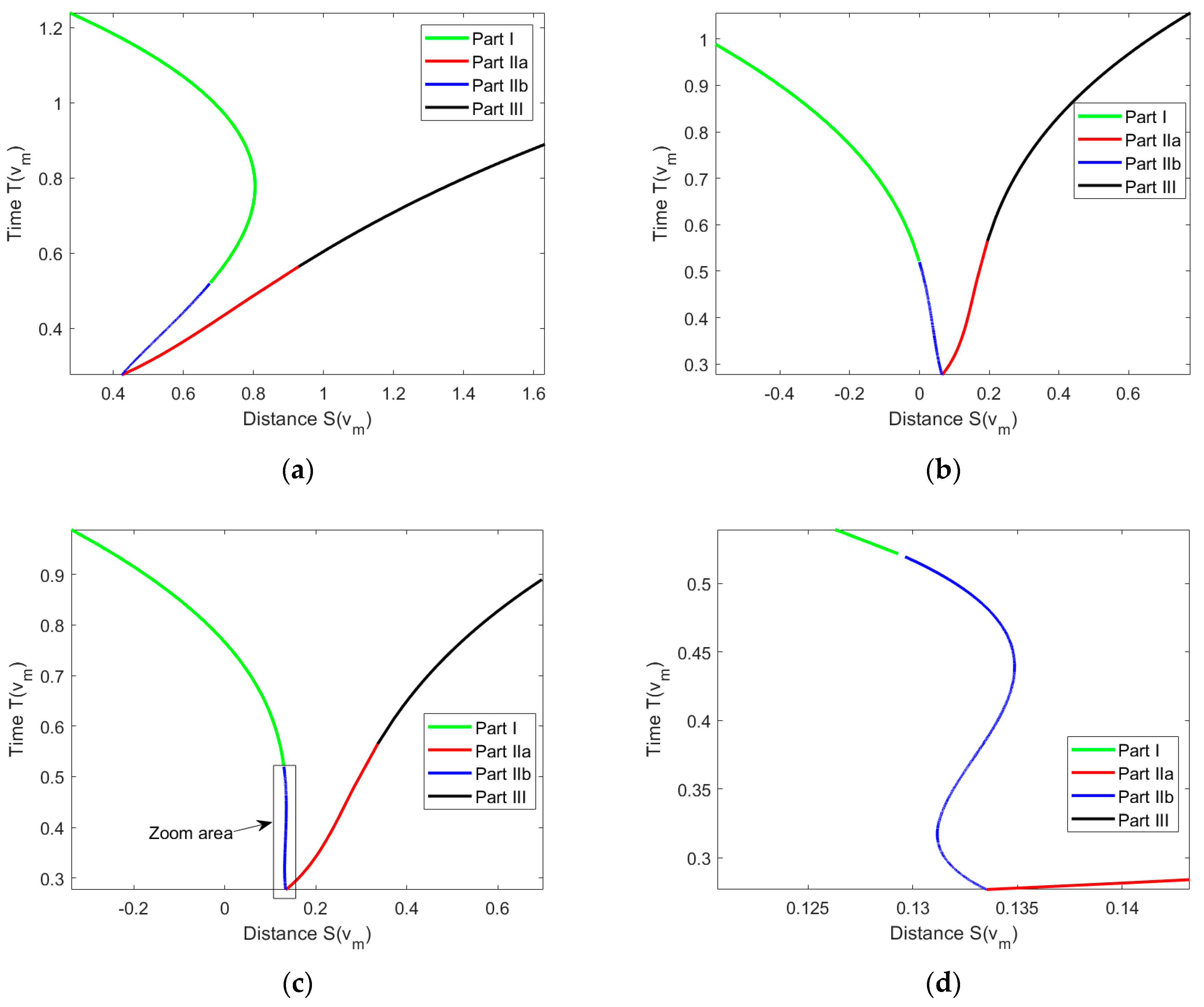
Example 3: Gap between Parts I and III, Parts IIa or IIb are needed.
Initial and final conditions: . We use the same accelerations as in Example 1 but shift the velocities by −11.5. For Parts I and III, the remarks given in Examples 1 and 2 are still valid; see Figure 10. However, here, in both parts, the distance changes monotonously. This example shows that without using the constructions of Parts IIa or IIb, a certain range of distances (here, roughly from 1.4 to 3) might not be covered. In the example, Part IIa provides the better solution and we have not encountered an example of case A where Part IIb is best, but we do not have proof that this is always so.
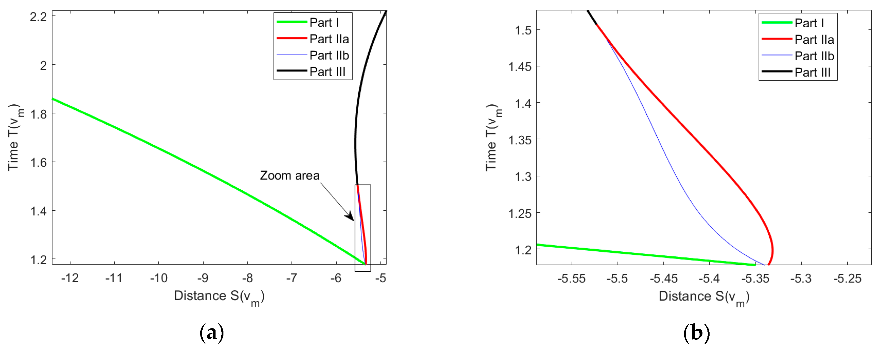
Example 4: Best solution is in Part IIa where the curve is “bulging”.
Initial and final conditions: . We use the same accelerations as in Example 1 but shift the velocities to the left by −17.2.
In this example, zooming shows that the red Part IIa curve “bulges” to the right (Figure 11b) (cf. similar examples in [22]). Therefore, there is a small interval of distances to the right by about −5.34 where Part IIa provides the best solution, ending at the S-value of the utmost right point of the red curve. This example demonstrates that for finding the best solution, it is, in general, not sufficient to just consider the interval of distances between the “end points” of the parts. If one considers the interval of S-values between the end points of the red curve, then on that interval, the Part I curve (green) is always better. Therefore, an approach working with “critical distances” as in [20] has its limits.
The examples given above show that a visualization using a parametric curve allows to easily create a variety of examples for finding counter-examples to conjectures one might have in mind. This has also been presented in [22] using a different parameterization. Using allows us to easily recognize in which part the best solution occurs. Moreover, the parameter has a direct meaning in the velocity–acceleration plane. One might be inclined to look for further patterns to see in advance which part provides the best solution, but even this small set of examples shows the variability. We will make no further distinctions but just compute the solution(s) provided by each part and take the best one (this approach is also used in [22]). We consider this as a sound compromise between complexity (comprehensibility) on the one hand and computational effort on the other hand. We find the best solution within the solutions provided by Parts I–III by inserting the given distance in Equations (7)–(10) and computing . As we will see in the next section, this requires finding the roots of polynomials. For each solution candidate, it is checked whether is admissible (real and within the allowed range). For the admissible ones, one computes the times and chooses the solution with lowest time. If or , one sets resp. and inserts a phase with constant (minimum or maximum) velocity.
- Case B: and ,
In this case, E lies “left of” A in the sense that E lies on a square root curve (open to the right) left of the square root curve (open to the right) that the point A lies on. We can proceed in the same way as we did in case A and have, again, four parts, as shown in Figure 12.
Again, with Part I resp. III, we can realize arbitrarily small resp. large distances going via intermediate velocities . Arguing as in case A, we obtain for Parts I and III the same formulae as in (7) and (8) resp. (11) and (12), but the ranges for are different for Part I and for Part III . The formulae for Parts IIa and IIb are different and provided below.
We omit examples for this case since they provide no new insights. The procedure for computing the best solution follows the same lines as the one described in case A.
- Case C: and , and
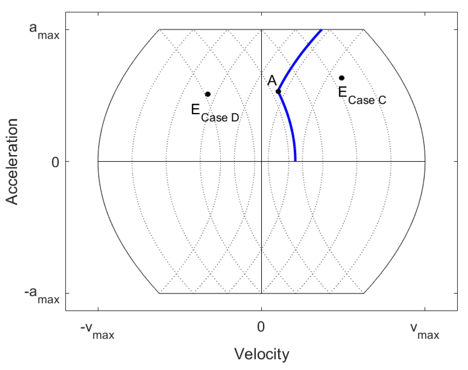
In this case, E lies “right of” A in the sense that E lies in the area right of or on the square root curve through A open to the right, and right of or on the square root curve through A open to the left (Figure 13).
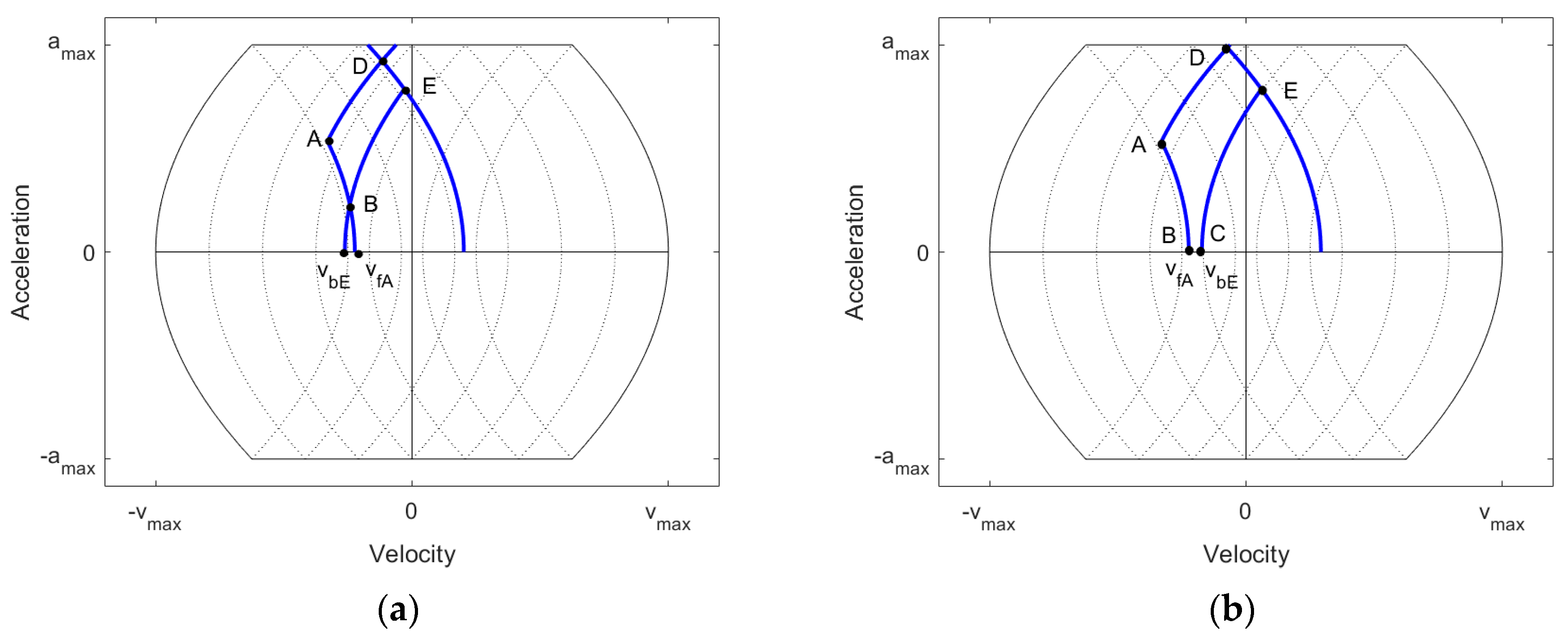
We split this case up into two sub-cases ( and ) that need partially different treatments. The sub-cases are shown in Figure 14. In the first sub-case (left), we have a closed curved quadrilateral ABED, whereas in the second one (right), we have a curved pentagon, ABCED. Note that in the first sub-case, there might also occur a curved pentagon when is reached, but this does not require a further distinction.
- Sub-Case Ca:
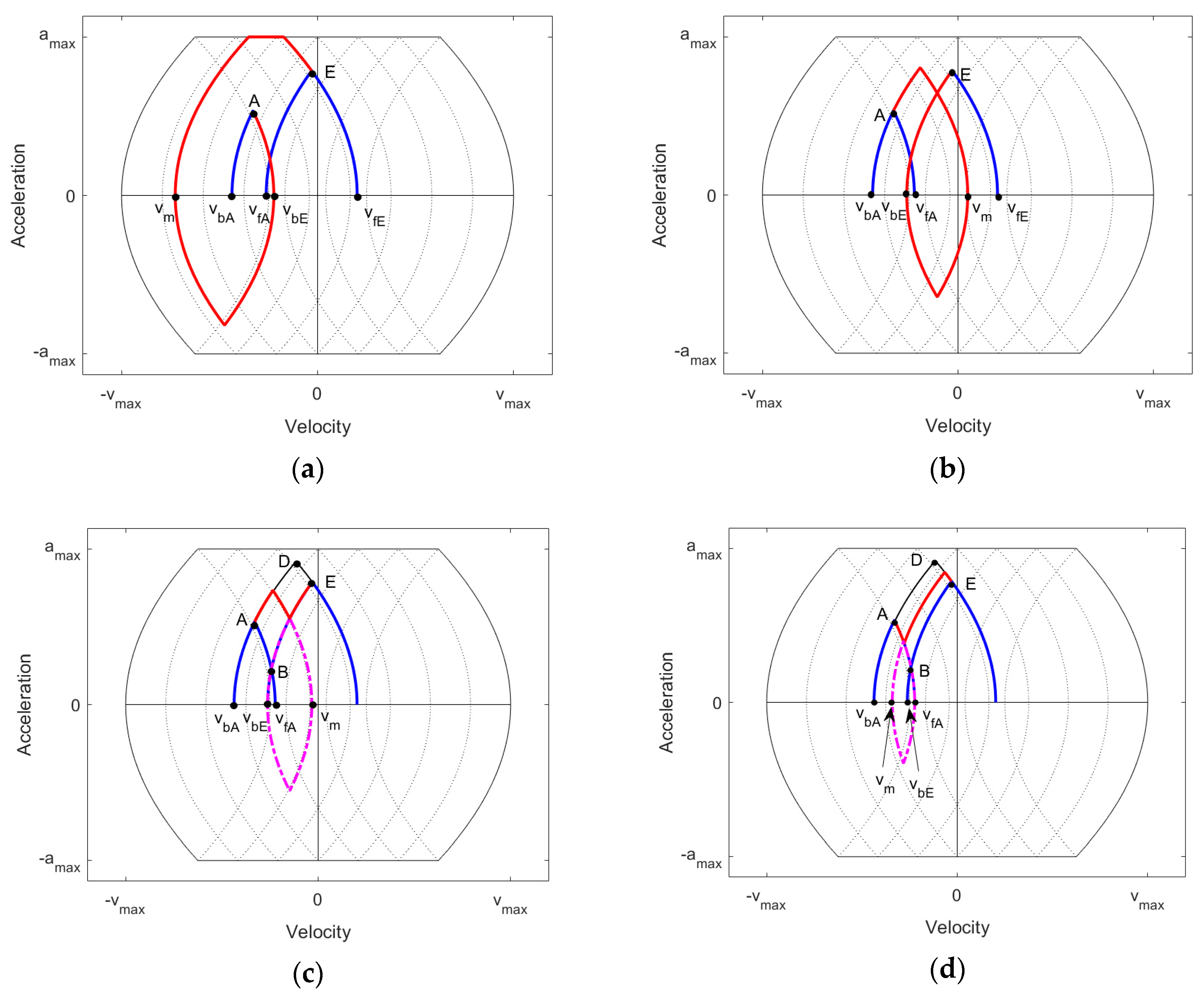
As in case A, we split up the construction of solutions for all distances into different parts, as shown in Figure 15. With Part I resp. III, we can realize arbitrarily small resp. large distances going via intermediate velocities resp. . If equality holds, then Part I and Part III provide the same point and, hence, the same distance Δs. Therefore, Parts I and III already cover all distances but do not necessarily provide the shortest time. Some distances can be realized better by going directly within the curved quadrilateral ABED using the sequence , , in Part IIa or the sequence , , in Part IIb (see Figure 15c,d). We will give an example for this situation below.
Arguing as in case A, we obtain the following formulae for distances and times:
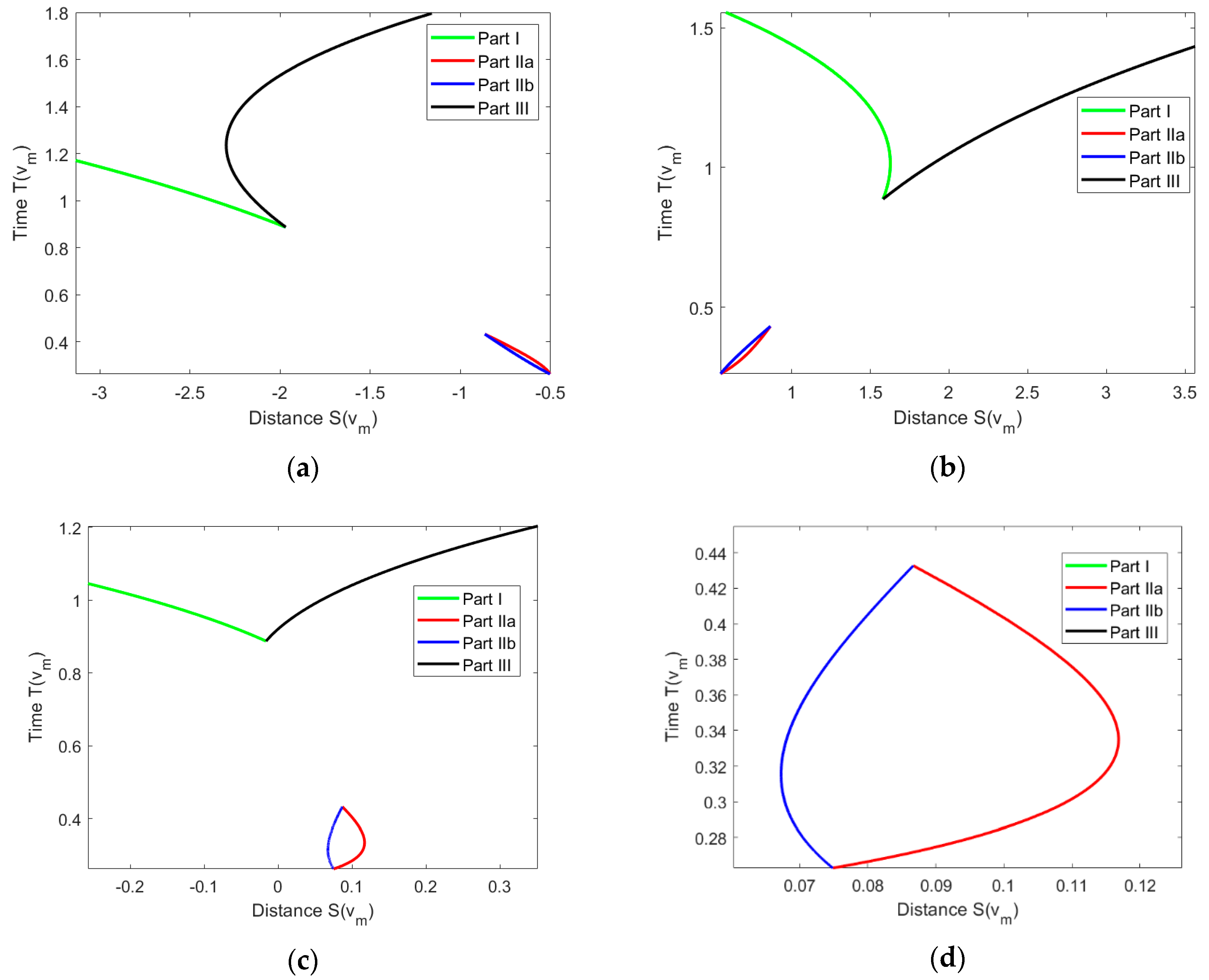
We provide some examples that give an insight into the variability of situations. We use the same values for the restrictions as in the examples given for Case A, i.e., , , . We have, again, one set of initial and final conditions and shift this in the v-direction. The values used for producing Figure 16 are: .
Example 1: Shift = 0, i.e., we use exactly the data given above.
Example 2: Shift = 4, i.e., we use: .
We recognize that the parts are no longer connected, but there are two “connectivity components”, Parts I/III and IIa/b. It can also be seen that Parts I and III provide solutions for all distances, but for the distances for which Parts IIa and IIb are applicable, they provide shorter times. In example 1, Part IIb is better than Part IIa, and in example 2, it is the other way around.
Example 3: Shift = 2.2, i.e., we use: .
In this example, we also recognize the disconnectedness. In addition, we see that both the red curve (Part IIa) and the blue curve (Part IIb) “bulge”. Part IIb provides the shortest solution within a range of distances from about 0.068 to about 0.074, whereas for Part IIa, this holds for a range from about 0.074 to about 0.116. This again shows that an approach considering different cases only between the distances reached at the boundary points of the parts cannot always provide the best solution.
- Sub-Case Cb:
This case is depicted in Figure 14b. Regarding Part I resp. III, the same holds as was stated for sub-case Ca, i.e., we can realize arbitrarily small resp. large distances going via intermediate velocities, but here, resp. (see Figure 17a,b). Moreover, if equality holds, then Part I and Part III do not provide the same point and, hence, the same distance Δs.
In order to guarantee the continuity of covered distances, we again include two other parts called Part IIa and IIb, using the sequence , , in Part IIa and the sequence , , in Part IIb (see Figure 17c,d). In Part IIa, the motion curve starting at A moves up in the direction of D beyond the point F, then moves down to a point on the curve CE and then up to E (see Figure 17c). This is much the same as shown in Figure 15c for the previous sub-case Ca, but note that now, the motion curve must go beyond F (otherwise one would need a sequence with three changes in jerk instead of two). In Part IIb, the motion curve starting at A moves down in the direction of B, then moves up to a point on the curve DE (which lies above the point G) and then down to E (see Figure 17d). We checked that all possible distances are covered by using continuity: If in Part I we choose , then we obtain the motion curve ABGE. This is also the motion curve one obtains in Part IIb when one goes down to the point B. At the other “end” of Part IIb, one obtains the motion curve ADE (i.e., going down by 0). This is also the motion curve one obtains in Part IIa when one goes up from A to D. At the other “end” of Part IIa, one obtains the motion curve AFCE. We also obtains this motion curve when we choose in Part III. Therefore, Parts IIa and b fulfill the purpose to continuously connect Parts I and III. As we will see in the examples, in this sub-case, the special situation might occur that we need both Parts IIa and IIb to have a full coverage of all distances, whereas in the other cases considered so far, only one of the parts was needed for this purpose.
The formulae for distances and time are the same as in the previous sub-case (i.e., Equations (19)–(26)) but the ranges for are different. Therefore, we just provide these ranges:
We provide some examples that give an insight into the variability of situations and the specifics of this sub-case. We use the same values for the restrictions as in the examples given for case A, i.e., , , . We have, again, one set of initial and final conditions and shift this in the v-direction: .
Example 1: Shift = 0, i.e., we use exactly the data given above (Figure 18a).
In this example, there is a gap between Parts I and III. Only Part IIa is needed to fill the gap. It also provides the shortest time where it is valid. One can see how one goes continuously from Part I via IIb and IIa to III as described above.
Example 2: Shift = −1.3, i.e., we use: (Figure 18b).
Here, both parts IIa and IIb are needed to cover all possible distances. For a certain distance, there is only one part that covers that distance and is, hence, automatically the best one.
Example 3: Shift =−1.05, i.e., we use: (Figure 18c).
This example looks, at first, similar to example 2, but when one zooms into the interesting area, one can recognize that for some distances covered by Part IIb (blue), there is also a coverage by Part IIa with a shorter time. Moreover, for some distances (e.g., 0.132), there are even three solutions within Part IIb, one of them having the shortest time. This again shows the variability of situations.
- Case D: and , or
This case is illustrated in Figure 19. Case D is the easiest one since it can be completely reduced to the GG situation by a combination of embedding and extension and we just need Parts I and III. Figure 19 shows situations when both of the two velocity conditions are fulfilled, but it is easy to check that nothing changes when only one of them holds. Consider the GG task for going from to via a . If one extends this by going from A to and cuts off the part going from E to , one obtains a motion curve from A to E with a certain distance. Making smaller and inserting a phase with velocity enables us to realize arbitrarily small values for Δs. Similarly, the red motion curve can be constructed from the GG task going from to via a . Again, making larger and inserting a phase with velocity enables us to realize arbitrarily large values for Δs. Since for and we obtain the same motion curve, we continuously cover all distances.
We obtain the same formulae for distances and times as for Parts I and III in Case Ca, i.e., Equations (19), (20), (23), (24) also hold in this case. Since there are no remarkable special situations occurring in this case, we give no examples.
5. Implementation and Validation with MATLAB®
In both the GG and the BB situations, beside splitting into several cases, which is easy to implement, the main task consists of solving an equation. In GG and in Parts I and III of the BB cases, the equation is of the type:
where is unknown and the distance and the velocities are given. The equations for Parts IIa and IIb in the BB situation (9), (10), (15), (16), (21) and (22) can be rewritten in the form:
We abbreviate the difference on the right hand side as .
We split up Equation (28) into sub-cases depending on whether the maximum acceleration is reached going from to resp. from to (cf. Equations (1) and (2)):
An analogous set of equations can be produced for (29) using minus instead of plus between the two parts. Moreover, a closer investigation of the interval where lies in Parts IIa and IIb shows that sub-case (33) does not occur, so when considering Equation (29), we can restrict ourselves to (30)–(32). Available numerical equation solvers for (28) and (29) normally find, at most, one solution and then stop. Therefore, we transform the equations symbolically into problems where all zeros of polynomials are to be found. For doing this, we first remove the absolute values by making a further distinction between the cases and (the overlap at equality does not matter). For example, in case (α), we write for . Using a Computer Algebra System (here, Maple®), one can then reduce the task of solving the equations (30)–(32) to find the roots of polynomials of degree 4 and one obtains even a symbolic solution for (33).
We first consider the equation . The polynomials for Equations (30)–(32) are given in Table A1 (Appendix A) in form of lists of coefficients (starting from the largest power) and the solutions for Equation (33) are given directly. If we consider instead the equation , we obtain only polynomials for the modified Equations (30)–(32), as shown in Table A2 (Equation (33) does not occur as stated above). Once all zeros z of the polynomials for the (modified) Equations (30)–(32) have been found using a polynomial root solver (here: MATLAB®), the solutions for Equations (30)–(32) for both equations and can be found according to Table A3 (provided by the Computer Algebra System).
All solution candidates are then further filtered:
- Only the real solutions (not the complex ones) are taken.
- It is tested whether the solutions fulfill the case conditions in (α) resp. (β).
- It is tested whether the solutions fulfill the requirements of Equations (30)–(33) regarding reaching the maximum/minimum acceleration.
- Not all zeros of the polynomial might solve the original equation (only the implication that all solutions of the equation can be found using zeros of the polynomials and the computations given in Table A3 holds in general; there is no equivalence relationship). Therefore, all zeros are tested (by insertion) and only those ones fulfilling the equation are kept.
Only those solutions that pass the tests are then used for further processing. This algorithm is described semi-formally in pseudo-code in Algorithm 1.
| Algorithm 1. Solving (resp. ). |
| Input: |
| Output |
| 1. If case = α Then |
| 2. Compute the zeros of polynomial (30) in Table A1 (resp. A2) listed under (α) |
| 3. according to Table A3 listed under (α) |
| 4. do |
| 5. If End If |
| 6. If not End If % Not case α |
| 7. If not End If % necessary condition for (30) |
| 8. If not End If % equation not solved |
| 9. End For |
| 10. Do the same (lines 2–9) for polynomials (31) and (32) adapting the inequalities in line 7 |
| 11. directly from (33) in Table A1 (not applicable for ) |
| 12. If applicable Then Do the same as in lines 4–9, adapting the inequalities in line 7 End if |
| 13. else if case = β Then |
| 14. Do the same as in case α now using the polynomials/expressions listed under case β in Table A1 (resp. A2) |
| 15. End If |
| 16. Return % might be the empty set |
If we have the BB task, we first determine which of the cases, A to D, is applicable (or rewrite the problem by changing the direction of distance). In the respective case, we determine the solutions for an equation of type for Parts I and III and the solutions for an equation of type for Parts IIa and IIb as described above. Note that even for Parts I and III where we can relate the BB task to a GG task by embedding or extension, we cannot simply use an algorithm for the GG task since we have to take into account the restrictions on the interval where must lie. We have to determine the zeros of, at most, 12 polynomials of degree 4 (four parts with three polynomials each at most). Then, we additionally check whether the solutions for are within the given range for the respective part (the ranges are given in the equations above) and drop those who are not. If or , we insert a phase with constant velocity. We then compute the lengths for the different time intervals in the seven-segment profile and sum these up. The candidate with the lowest sum is then the best one within the set of all candidates considered. The algorithm is described semi-formally in Algorithm 2.
| Algorithm 2. Computing the time intervals and signs for the 7-segment profile. |
| Input: |
| Output |
| Then |
| 3: End If |
| 4: If case = A Then |
| 5: Call Algorithm 1 according to Equation (7) |
| returned |
| in Equation (7) is not fulfilled Then |
| 9: Else |
| End If % Take into account restriction on v |
| 11: Compute time vector and sign vector |
| 12: End if |
| 13: End For |
| 14: Call Algorithm 1 according to Equation (8) and perform lines 6–13 |
| according to Equation (9) and perform lines 6–13 |
| according to Equation (10) and perform lines 6–13 |
| 17: Else If case = B |
| 18: Execute lines 5–16 using the equations of case B |
| 19: Else If case = Ca |
| 20: Execute lines 5–16 using the equations of case Ca |
| 21: Else If case = Cb |
| 22: Execute lines 5–16 using the equations of case Cb |
| 23: Else If case = D |
| 24: Execute lines 5–16 using the equations of case D |
| 25: End If |
If we have a GG task, we can determine in advance which one of the Equations (30)–(33) is applicable and determine whether we have case (α) or (β) (we omit the details). Therefore, we would have to find the roots of at most one polynomial.
Regarding validation, we have to state first what we intend to validate. Since the presented algorithm logically covers all possible situations by the continuity argument we explained in the previous section, theoretically, there is no necessity for validation otherwise than checking for a mistake in the argumentation that might come up during test runs. What certainly needs validation is the implementation of the algorithm, particularly regarding numerical issues such as cancellation effects (accuracy). Moreover, for checking the algorithm’s suitability for online trajectory planning, it is also important to investigate efficiency, i.e., the time necessary for finding the solution. Our accuracy and efficiency check was performed by having a huge number of test runs with randomly generated data covering all the cases and parts described in Section 4. We used the following scheme:
- We first prescribe upper boundary values for , called , and the largest distance is considered. We choose 100 for each (units: m/s3, m/s2, m/s, m) for our test runs to allow for a larger range but this is a bit arbitrary.
- Within the interval , we generate a random value for and proceed analogously for , . Moreover, for , we do so randomly.
- Within the area in the velocity–acceleration plane that is bounded by the horizontal lines at and the left and right square root curves shown in Figure 3, we choose values for and randomly.
- Once the configuration has been generated randomly this way, a test run for computing the best function is performed and it is checked whether the solution really gives the prescribed final velocity and acceleration and the distance Δs within a certain margin of error. If the error is larger than 10–7, the configuration producing it is recorded for further investigation.
Given this scheme, we made several runs with 107 random configurations which took about 40 min each (depending on whether the profiler in MATLAB was turned on or off). During the first test runs, we encountered, a few times, the situation that no solution was found, which is in contradiction with the logical argumentation in Section 4. The reasons were, as already assumed, of numerical origin and of two different kinds. In the first type of situation, the solutions were at border points between different parts. Consider, for example, case B: If there is a solution very close to the border for between Part IIa and Part IIb (i.e., ), then it might not be accepted in Part IIa because it is required there that . By simply allowing equality here (which in theory means one has an overlap between Parts IIa and III), one can avoid this problem. One could also allow a small overlapping ε-interval here. The second type of situation where no solution was found had its origin in the error margin for the distance in the computation of candidates (roots of the polynomials). By enlarging the error margin, this type of problem could be avoided in the subsequent runs. Since, in the final solution, the distance is again checked, this does not lead to the acceptance of solutions with errors above a specified value. Actually, since distances are computed using Equations (30)–(33), stated above in this section, we might have typical cancellation effects when and or and have nearly the same absolute value.
We performed a test run with 108 configurations, which provided a solution for all configurations, so the numerical remedies reported above seem to work. Table 2 gives information on errors. The maximum error in Δs was 6.57 × 10⁻⁶ and there were only 15 configurations with errors in Δs of more than 1 × 10⁻⁷. Therefore, we conclude that the implementation provides acceptable results for realistic situations regarding the values for and .
Table 3 provides information on the case and part coverage. It shows that all cases and parts were sufficiently covered except for Part IIb in cases A and B (in case D, Parts IIa and IIb do not occur; see Section 4). In earlier test runs with less configurations, it was nearly always the case that there was no example for Part IIb in cases A and B, and we conjectured already in Section 4 that Part IIb might be unnecessary. A closer look at the configurations that led to the 12 entries for Part IIb in cases A and B revealed that, again, this is a numerical effect. As is shown in Figure 10, if the solution point is very close to the “meeting point” of the curves for Parts IIa, IIb and III, it might happen that because of round-off errors, IIb gives a lower time value than IIa, although zooming in shows that Part IIb is above Part IIa. Practically, this does not really matter since the solutions provide nearly the same time. Therefore, we still stick to our conjecture that in cases A and B, Part IIb never contains the best solution.
Regarding efficiency, we wanted to investigate whether the computation of the best function can be performed within a controller cycle which might be 1 ms (cf. [12]) or less, and for very fast controllers, even 100 μs. In our computations, we used a desktop PC with a Xeon E5-1630v4 processor with 3.7 GHz.
It is not straightforward to generate valid efficiency data when running MATLAB functions. As stated in Mathwork’s own performance white paper [23], there is much “noise” to be taken into account, which might lead to considerable variation of times. This noise includes scheduling of processes and threads by the operating system and use of different memory caches. Moreover, the just-in-time compiler of MATLAB compiles a function once and uses then the compiled version. The variation can be made visible by running the best function with a fixed configuration several times, such that the computational work is identical. This gave values between a few milliseconds and a few hundred microseconds. We took this into account by repeating the computation for the same configuration several times and then taking the lowest value. We measured the times for the best function finder for 100,000 configurations, each repeated 1000 times, which provides a good coverage of all cases and parts. The maximum time was 303 μs. The result already shows that a run of the best function finder can be performed with a cycle time of 1 ms without any problem. However, there is even considerable potential for improvement. One of the main tasks in the best function finders is the computation of roots of the 12 polynomials of degree 4. In a test run with 1,000,000 configurations with 20 repetitions each, we measured an average time of 156 μs for computing the roots of the 12 polynomials. MATLAB’s roots function is a general root-finding function for polynomials of an arbitrary degree. For polynomials of degree 4 (also called “quartics”), there are many more efficient special solvers available. For solving a quartic accurately and efficiently, Orellana and De Michele [24] needed less than 0.5 μs on a dual-core i7 processor with 3.3 GHz. This means that by using such a specific solver, we can reduce the effort for root finding to about 6 μs (12 polynomials). That would cut the “worst case” time for computing the best function of about 303 μs by half. Moreover, our current MATLAB code contains overhead for providing additional information, and the code is split up into several small functions for making it better readable. Modern compilers contain optimizers that try to reduce the overhead when actually producing the executable code, e.g., by so-called “inlining”, where calls to “small functions” are substituted by inserting the code of the functions into the calling function. Orellana and De Michele [24] showed that by using a certain optimizer option, they could reduce the time needed by about half. This indicates that the time needed for computing the best function could even be brought well below 100. This is comparable with the time reported in [12] for the worst case (540 for six axes) and in [19] as average (74 for one axis). Sidobre and Desormeaux [22] even achieved 2.5, but the three-variable Newton method they applied after first obtaining an approximation did not always provide the optimal solution. The most important criterion for online trajectory generation is not the absolute time as long as the computation can be performed within one controller cycle.
6. Conclusions
In this contribution, we investigate how a fast motion function can be found when restrictions for jerk, acceleration and velocity, initial and final values for velocity and acceleration and the distance are given. Our approach applies a seven-segment motion profile with piecewise constant jerk, which was already considered by other authors. We developed an algorithm for computing such a profile which considers only four major cases and, hence, has a manageable complexity. We investigate these cases systematically in the velocity–acceleration plane, which provides an easily understandable visual explanation. The investigation showed that there are often several seven-segment profiles fulfilling the condition differing considerably in execution time. We take the best one, whereas the algorithm by Ezair et al. [19] leads to just one of them. Since (like Sidobre/Desormeaux [22]) we do not have mathematical proof that there are no other seven-segment profiles with shorter times, we only claim to have a “fast” solution, not necessarily an “optimal” one. Moreover, a continuity argument proved that we cover all possible distances, whereas in the work by Sidobre and Desormeaux [22] treating the same problem, only a brief explanation but no proof is given.
We implemented our algorithm in MATLAB, where we reduced the computation essentially to the finding of roots of up to 12 polynomials of degree 4, which can easily be re-implemented. A large test run with 108 configurations showed that a solution was always found and all cases as well as all parts were covered satisfactorily. This also supports our claim of full coverage of all possible situations. Moreover, our timing experiments showed that our algorithm is suitable for online trajectory generation. Although finding the zeros of up to 12 polynomials makes our algorithm a bit slower than algorithms for special situations (such as [12]), the additional cost is small since very fast solvers for quartics are available.
There are also clear limitations to the approach using a seven-segment profile. Since the jerk function is piecewise constant, the discontinuity might lead to unwanted vibrations. As stated in the literature review, for special situations such as RR (“rest-to-rest”), smoother functions have been designed. This deficit of the seven-segment approach might be reduced by working with a 15-segment profile with continuous jerk. A feasible way for finding such a profile in the general BB task might be to generalize the approach developed in this contribution. A further limitation of the seven-segment approach is that it does not handle variable constraints but only constant ones, and the constraints are assumed to be symmetric, although it would be possible to modify our approach in order to include asymmetric constraints.
We have not tested the applicability of seven-segment profiles experimentally since this has already been performed by other authors (e.g., [12,22]), on whom we rely. In real applications such as robotics, the situation we investigated in this article is only one problem among many. Further considerations are necessary when there are several drives that need coordination or when restrictions change and one has to turn the initial state into an admissible one first. One can find strategies for this in [12,19,20,25].
Funding
This research received no external funding.
Institutional Review Board Statement
Not applicable.
Informed Consent Statement
Not applicable.
Data Availability Statement
Not applicable.
Conflicts of Interest
The author declares no conflict of interest.
Appendix A

Table A1.
Polynomials and solutions for .
| List of Coefficients for (30)–(32) Resp. Solutions for (33) | |
|---|---|
| Case (α) | |
| (30) | |
| (31) | |
| (32) | |
| (33) | |
| Case (β) | |
| (30) | |
| (31) | |
| (32) | |
| (33) |
Table A2.
Polynomials and solutions for .
| List of Coefficients for Modified (30)–(32) | |
|---|---|
| Case (α) | |
| (30) | |
| (31) | |
| (32) | |
| Case (β) | |
| (30) | |
| (31) | |
| (32) |
Table A3.
Solution candidates for .
| Case (α) | |
| (30) | |
| (31) | |
| (32) | |
| Case (β) | |
| (30) | |
| (31) | |
| (32) |
References
- Biagiotti, L.; Melchiorri, C. Trajectory Planning for Automatic Machines and Robots; Springer: Berlin/Heidelberg, Germany, 2008. [Google Scholar]
- Carbone, G.; Gomez-Bravo, F. (Eds.) Motion and Operation Planning of Robotic Systems; Mechanisms and Machine Science 29; Springer: Berlin/Heidelberg, Germany, 2015. [Google Scholar]
- Gasparetto, A.; Boscariol, P.; Lanzutti, A.; Vidoni, R. Path Planning and Trajectory Planning Algorithms: A General Overview. In Motion and Operation Planning of Robotic Systems; Carbone, G., Gomez-Bravo, F., Eds.; Springer: Berlin/Heidelberg, Germany, 2015; pp. 3–27. [Google Scholar]
- VDI (Ed.) Guideline 2143: Motion Rules for Cam Mechanisms; Theoretical Fundamentals (German); Beuth Verlag: Berlin, Germany, 1980. [Google Scholar]
- Kröger, T.; Wahl, F.M. Online Trajectory Generation: Basic Concepts for Instantaneous Reactions to Unforseen Events. IEEE Trans. Robot. 2010, 26, 94–111. [Google Scholar]
- Macfarlane, S.; Croft, E.A. Jerk-bounded manipulator trajectory planning: Design for real-time applications. IEEE Trans. Robot. Autom. 2003, 19, 42–52. [Google Scholar] [CrossRef] [Green Version]
- Liu, H.; Liu, X.; Wu, W. Time-optimal and jerk-continuous trajectory planning for robot manipulators with kinematic constraints. Robot. Comput. Integr. Manuf. 2013, 29, 309–317. [Google Scholar] [CrossRef]
- Lin, J.; Somani, N.; Hu, B.; Rickert, M.; Knoll, A. An Efficient and Time-Optimal Trajectory Generation Approach for Waypoints under Kinematic Constraints and Error Bounds. In Proceedings of the IEEE/RSJ International Conference on Intelligent Robots and Systems (IROS), Madrid, Spain, 1–5 October 2018. [Google Scholar]
- Shen, P.; Zhang, X.; Fang, Y. Complete and time-optimal path-constrained trajectory planning with torque and velocity constraints: Theory and applications. IEEE/ASME Trans. Mechatron. 2018, 23, 735–746. [Google Scholar] [CrossRef]
- Penin, B.; Giordana, P.R.; Chaumette, F. Minimum-time trajectory planning under intermittent measurements. IEEE Robot. Autom. Lett. 2019, 4, 153–160. [Google Scholar] [CrossRef] [Green Version]
- Shiller, Z. Off-line and On-Line Trajectory Planning. In Motion and Operation Planning of Robotic Systems; Carbone, G., Gomez-Bravo, F., Eds.; Springer: Berlin/Heidelberg, Germany, 2015; pp. 29–62. [Google Scholar]
- Kröger, T. On-Line Trajectory Generation in Robotic Systems; Springer: Berlin/Heidelberg, Germany, 2010. [Google Scholar]
- SEW Eurodrive. Manual Program. Module MultiMotion; SEW: Bruchsal, Germany, 2010. [Google Scholar]
- Wang, H.; Wang, H.; Huang, J.; Zhao, B.; Quan, L. Smooth point-to-point trajectory planning for industrial robots with kinematical constraints based on high-order polynomial curve. Mech. Mach. Theory 2019, 139, 284–293. [Google Scholar] [CrossRef]
- Fang, Y.; Hu, J.; Liu, W.; Shao, Q.; Qi, J.; Peng, Y. Smooth and time-optimal S-curve trajectory planning for automated robots and machines. Mech. Mach. Theory 2019, 137, 127–153. [Google Scholar] [CrossRef]
- Trigatti, G.; Boscariol, P.; Scalera, L.; Pillan, D.; Gasparetto, A. A look-ahead trajectory planning algorithm for spray painting robots with non-spherical wrists. In Proceedings of the 4th IFToMM Symposium on Mechanism Design for Robotics, Udine, Italy, 11–13 September 2018; pp. 235–242. [Google Scholar]
- Liu, S. An On-line Reference-Trajectory Generator for Smooth Motion of Impulse-Controlled Industrial Manipulators. In Proceedings of the 7th International Workshop on Advanced Motion Control, Maribor, Slovenia, 3–5 July 2002; pp. 365–370. [Google Scholar]
- Haschke, R.; Weitnauer, E.; Ritter, H. On-line planning of time-optimal, jerk-limited trajectories. In Proceedings of the IEEE/RSJ International Conference on Intelligent Robots and Systems, Nice, France, 27–31 October 2008; pp. 3248–3253. [Google Scholar]
- Ezair, B.; Tassa, T.; Shiller, Z. Planning high order trajectories with general initial and final conditions and asymmetric bounds. Int. J. Robot. Res. 2014, 33, 898–916. [Google Scholar] [CrossRef]
- Broquère, X. Planification de Trajectoire Pour la Manipulation D’objets et L’interaction Homme-Robot. Ph.D. Thesis, Université Paul Sabatier Toulouse III, Toulouse, France, 2011. [Google Scholar]
- Broquère, X.; Sidobre, D.; Herrera-Aguilar, I. Soft motion trajectory planner for service manipulator robot. In Proceedings of the IEEE/RSJ International Conference on Intelligent Robots and Systems, Nice, France, 22–26 September 2008; pp. 2808–2813. [Google Scholar]
- Sidobre, D.; Desormeaux, K. Smooth cubic polynomial trajectories for human-robot interactions. J. Intell. Robot. Syst. 2019, 95, 851–869. [Google Scholar] [CrossRef] [Green Version]
- McKeeman, B. MATLAB Performance Measurement; Mathworks: Natick, MA, USA, 2020. [Google Scholar]
- Orellana, A.G.; De Michele, C. Algorithm 1010: Boosting Efficiency in Solving Quartic Equations with No Compromise in Accuracy. ACM Trans. Math. Softw. 2020, 46, 20:1–20:28. [Google Scholar] [CrossRef]
- Desormeaux, K.; Sidobre, D. Online Trajectory Generation: Reactive Control with Return Inside an Admissible Kinematic Domain. In Proceedings of the International Conference on Intelligent Robots and Systems (IROS 2019), Macau, China, 4–8 November 2019. [Google Scholar]
Figure 1.
Seven-segment profile (a) for RR; (b) for BB—two segments with length 0.


Figure 3.
Switching between velocities: (a) positive acceleration; (b) negative acceleration.

Figure 4.
Examples for getting from to : (a) velocity–acceleration plane; (b) velocity over time.

Figure 5.
For and : (a) S over ; (b) T over S.

Figure 6.
Illustration of auxiliary functions.

Figure 7.
Case A. (a) Part I; (b) Part III; (c) Part IIa; (d) Part IIb.

Figure 8.
(a) No gap between Parts I and III, but Parts IIa or IIb are better; (b) zoom into area.

Figure 9.
(a) No gap between Parts I and III, Parts IIa or IIb are not needed; (b) zoom into area.

Figure 10.
(a) Gap between Parts I and III, Parts IIa or IIb are needed; (b) zoom into area.

Figure 11.
(a) Best solution is in Part IIa where the curve is “bulging”; (b) zoom into area.

Figure 12.
Case B. (a) Part I; (b) Part III; (c) Part IIa; (d) Part IIb.

Figure 13.
Positioning of A and E in cases C and D.

Figure 14.
(a) Sub-case Ca; (b) sub-case Cb.

Figure 15.
Case Ca. (a) Part I; (b) Part III; (c) Part IIa; (d) Part IIb.

Figure 16.
(a) Example 1; (b) example 2; (c): example 3; (d) example 3 with zoom.

Figure 17.
Case Cb. (a) Part I; (b) Part III; (c) Part IIa; (d) Part IIb.

Figure 18.
(a) Example 1; (b) example 2; (c) example 3; (d) example 3 with zoom.

Figure 19.
Case D.

Table 1.
Basic cases in the BB situation.
| Case | ||
|---|---|---|
| Case A | ||
| Case B | ||
| Case C | ||
| Case D |
Table 2.
Largest errors in a test run with 108 configurations.
| Run with Lower Bounds | |
|---|---|
| Max. error Δs | 6.57 × 10⁻⁶ (m) |
| Max. error vE | 4.67 × 10⁻¹² (m/s) |
| Max. error aE | 7.11 × 10⁻¹⁴ (m/s2) |
| Number of Errors in Δs > = 10−7 | 15 |
Table 3.
Coverage of cases and parts.
| Case A | Case B | Case Ca | Case Cb | Case D | |
|---|---|---|---|---|---|
| Part I | 10,561,715 | 10,563,034 | 1,085,981 | 9,209,731 | 13,996,250 |
| Part IIa | 727,205 | 728316 | 17,555 | 691,269 | 0 |
| Part IIb | 3 | 9 | 17,756 | 692,692 | 0 |
| Part III | 13,710,379 | 13,713,522 | 1,087,589 | 9,206,664 | 13,990,330 |
| Sum | 24,999,302 | 25,004,881 | 2,208,881 | 19,800,356 | 27,986,580 |
Publisher’s Note: MDPI stays neutral with regard to jurisdictional claims in published maps and institutional affiliations. |
© 2021 by the author. Licensee MDPI, Basel, Switzerland. This article is an open access article distributed under the terms and conditions of the Creative Commons Attribution (CC BY) license (http://creativecommons.org/licenses/by/4.0/).
Share and Cite
MDPI and ACS Style
Alpers, B. On Fast Jerk–, Acceleration– and Velocity–Restricted Motion Functions for Online Trajectory Generation. Robotics 2021, 10, 25. https://0-doi-org.brum.beds.ac.uk/10.3390/robotics10010025
AMA Style
Alpers B. On Fast Jerk–, Acceleration– and Velocity–Restricted Motion Functions for Online Trajectory Generation. Robotics. 2021; 10(1):25. https://0-doi-org.brum.beds.ac.uk/10.3390/robotics10010025
Chicago/Turabian StyleAlpers, Burkhard. 2021. "On Fast Jerk–, Acceleration– and Velocity–Restricted Motion Functions for Online Trajectory Generation" Robotics 10, no. 1: 25. https://0-doi-org.brum.beds.ac.uk/10.3390/robotics10010025
Note that from the first issue of 2016, this journal uses article numbers instead of page numbers. See further details here.