Autonomous Elbow Controller for Differential Drive In-Pipe Robots


Department of Electrical and Electronic Engineering, University of Manchester, Manchester M13 9PL, UK
*
Author to whom correspondence should be addressed.
Robotics 2021, 10(1), 28; https://0-doi-org.brum.beds.ac.uk/10.3390/robotics10010028
Submission received: 16 October 2020
/
Revised: 22 January 2021
/
Accepted: 27 January 2021
/
Published: 2 February 2021
(This article belongs to the Special Issue Advances in Robots for Hazardous Environments in the UK)
Abstract
:The inspection of legacy nuclear facilities to aid in decommissioning is a world wide issue. One of the challenges is the characterisation of pipe networks within them. This paper presents an autonomous control system for the navigation of these unknown pipe networks, specifically focusing on elbows. The controller utilises three low-cost feeler sensors to navigate the FURO II robot around 150 mm short elbows. The controller is shown to allow the robot to safely navigate around an elbow on all 39 attempts comparing that with the brute force method which only completed five of the nine attempts and damaging the robot. This shows the advantages of the proposed controller. A new metric (Impulse) is also proposed to compare the extra force applied to the robot over the time it is slipping in the elbow due to the errors in the drive unit speeds. Using this metric, the controller is shown to decrease the Impulse applied to the robot by Ns when compared to the brute force method.
1. Introduction
Nuclear decommissioning is forecast to cost the UK billion over the next 120 years [1]. One of the major challenges associated with it is the characterisation of the contents of legacy facilities [2]. A common feature within them is an extensive network of pipes which are of unknown geometry but have diameters between 50–150 mm. Currently, there is no way of inspecting this pipework without human intervention, which can be dangerous due to the unknown radiological contaminants inside them. An autonomous pipe inspection robot, FURO I, was proposed in [3], which could be used for such inspections, thus reducing the safety risks to human operators. This paper is an extension of that work, presenting the testing and development of a controller to allow the FURO robot to safely turn through an elbow.
1.1. Pipework
The pipework is reviewed in more detail to understand the operating environment for the control system being developed.
The pipe networks can consist of vertical and horizontal sections of pipe as well elbows and other junctions. The lengths of the networks can vary dramatically, from small sections of a few meters between gloveboxes to much larger drainage systems, which in some cases can have runs for miles [4,5]. Figure 1 shows a photo of the set of pipework in need of decommissioning inside an exemplar facility.
It is assumed that the facilities are constructed to industrial standards, which constrain the material choices for the pipework as well as features such as elbow radius, please see Appendix A, Pipe Standards for more details.
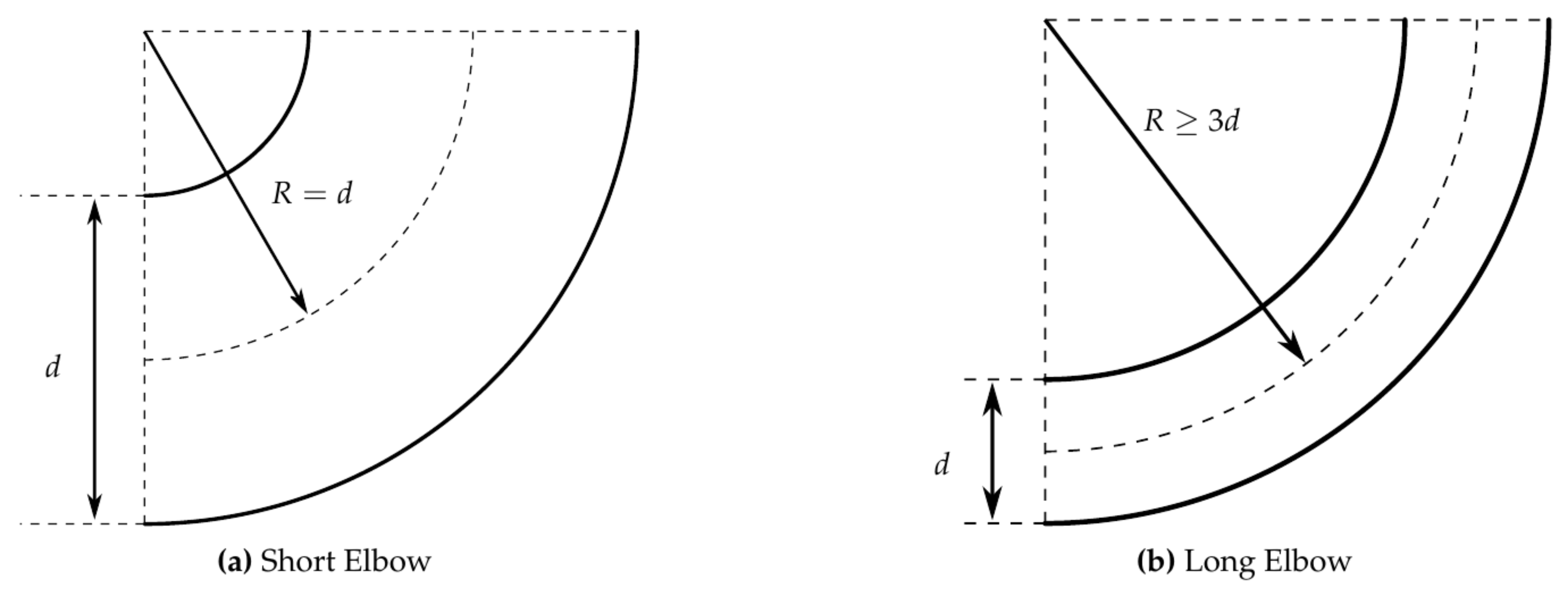
Elbows (or corners) can be classified into two types: long and short (Figure 2). A short elbow is the tightest bend within the pipework. It is defined as the radius of the curve (R) being equal to the diameter of the pipe (d). Note that R is specified at the centre of the pipe. A long elbow is defined as the radius of the curve being equal to or greater than three times the pipe diameter.
1.2. Pipe Inspection Robots
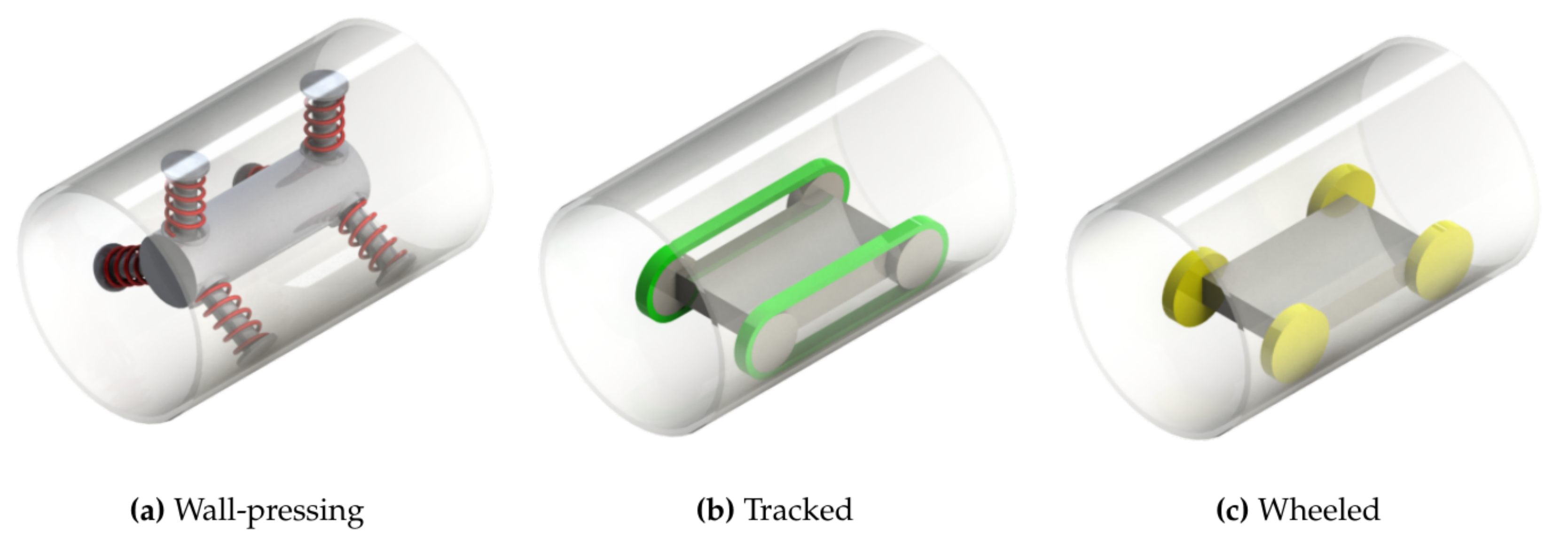
There are many challenges associated with pipe inspection and a wide number of robots have been constructed for various tasks. These robots are commonly classified into several categories: ‘Wall-Pressing’ (WP), ‘Pipe Inspection Gauge’ (PIG), Tracked, Wheeled, Walking, Inchworm and Spiral [6]. Additional types of pipe inspection vehicles exist such as snake robots. These are highly flexible and complex, making them able to overcome multiple obstacles and junctions [7]. Due to their complexity, they have many actuators meaning they require large amounts of energy to move and may struggle to form a stable platform for the sensors required for inspection. As the pipework has vertical sections as well as junctions, the focus for this paper is WP, Wheeled or Tracked robots, Figure 3. Those selected as WP are required to climb vertical sections of pipe first shown with the MOGRER [8] and FERRET-1 [9] robots in 1987. The focus on Wheeled or Tracked vehicles is due to the requirement of Differential Drive (DD), which is dictated by the need to navigate junctions [6].
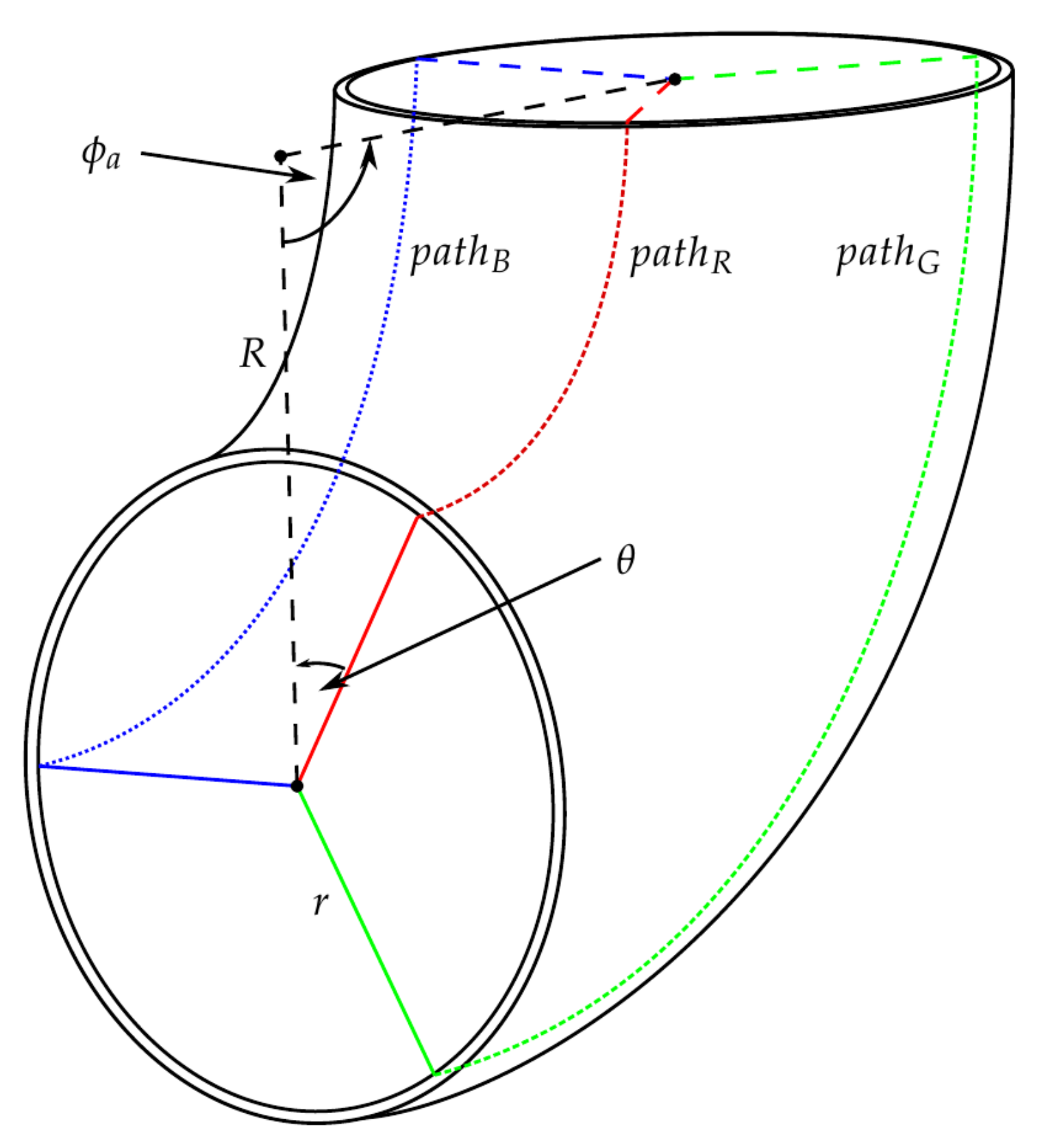
Despite WP, DD systems being commonly used [6,10,11] they have some limitations. One major challenge is calculating the speed of the wheels when turning through an elbow. Figure 4 shows three paths () of the drive units (DUs) of a DD, WP robot. It can be seen that these vary in length and this is dependent on various factors such as the corner direction (in relation to the robot), , the corner angle, and the major, R and minor, r radii of the corner. These path lengths dictate the required speed of each DU to be able to safely turn the corner and exit it at the same time. If these velocities are incorrect it causes additional forces to be applied to the robot, which can lead to damage and early fatigue, as well as this can also cause the robot to become lodged in the pipe. Most systems use a brute force (BF) method for cornering [12], i.e., there is no or little control on how to overcome junctions, the robot is driven as if it is in a straight section of pipe and the limitations of this are described above. In addition to this, Roh and Choi [6] found the current consumption was increased by when no control was used, making BF less efficient than controlled methods. Examples of systems that use BF to corner [13,14] will be discussed in further detail in this section.
Work has been completed on reducing the effect of the extra forces on the robot when using BF by making it compliant, to remove the need for a complex control system. Such as the Tracked robot from Nagase and Fukunaga [13], it requires only one motor for navigating elbows, vertical sections and variable pipe diameters. As it is not a Differential Drive it is unable to actively choose direction so it is unsuitable for navigating complex junctions.
Some Wheeled and Tracked systems use their design to allow them to corner. Both NIRVANA [15] and MRINSPECT VII [16] use multi-axis gear mechanisms that allow for the wheels to spin at different speeds, providing DD without the need of controlling individual motors. This solution contains very complex gear mechanisms that would be very difficult to miniaturise for small pipes making it unsuitable for this application. They also would be unable to select a direction at a junction such as a T-junction, due to not having independent DD.
A large amount of work on determining a suitable control action has been completed. Lee et al. [14] used a double actuated joint to force the drive unit to stick to the centre of the elbow. This method essentially still uses BF but tries to control the position of the robot inside the elbow with an extra actuator. Zhang et al. [17] and Chen et al. [18] both analysed the kinematics of a Wheeled robot to determine the wheel velocities. They provide a very complex solution to the problem and have no practical implementation. Zhang and Wang [19] determined the optimal posture for a track robot turning an elbow but do not use this to determine any control actions for the robot. These also all assume that the dimensions of the corner are known which is unsuitable for an unknown pipe network.
Fully autonomous pipe inspection robots such as FAMPER [10] require a pre-determined map of the pipe network such that it is not required to sense the corners ahead. This is demonstrated to work but for the use case of this research the pipe network is unknown, so this method would be unsuitable.
The described robots above are summarised in Table 1.
There are very few control methods that will work in networks with very little to no prior knowledge. The following section contains a review of the controlled cornering methods with WP, DD, Wheeled or Tracked robots where the elbow is considered to be unknown.
1.3. Control of Elbows
There are only a very limited number of systems that can controllably navigate unknown elbows. Their sensing methods for determining when in an elbow and then their control method is summarised in Table 2.
MRINSPECT v [20] proposes using pose sensing after its prediction of corner parameters, measuring the change in its orientation to determine when the robot has turned the corner. There is very limited information on whether this method is viable as it requires a knowledge of the elbow angle such that the pose can be sensed for that change. As the pipework in question is unknown, this is not suitable for this project. Lee et al. [21] also used an Inertial Measurement Unit (IMU) to detect when the robot is in an elbow. By reviewing the change in angular velocity, they can determine when the robot has exited the elbow. This work, despite being accurate, is unsuitable as the robot needs to have exited the corner so the end of the corner and the direction can be detected. This would mean the robot would have already completed the corner before the control action is calculated.
The IPR-D300 [11] uses ultrasonic (US) sensors to detect the wall distance from the drive unit (DU). When the distance passes a pre-set threshold, the motor speed of that DU is halved. This offers some aid in turning; however, it is a very inaccurate method of sensing and would still lead to large amounts of extra force being exerted on the robot. They show images of the robot successfully navigating an elbow but this led to a track derailing which is likely an effect of the increased forces.
1.4. Paper Overview
With this paper, we present and test a control methodology for an Autonomous Elbow Controller (AEC). The controller is tested on real world hardware, which is presented in Section 2. The control methodology is then presented in Section 3 and the experimental setup to test the AEC on the robot is described in Section 4, finally the results of the experiments are analysed and discussed in Section 5.
The contribution of this paper is the development of an autonomous control method for navigating around unknown pipe elbows, using low-cost and scalable feeler sensors making this system applicable to a large range of pipework sizes.
2. Hardware
This section contains an overview of the robot and the sensing suite being used for the development of the AEC.
- FURO II:
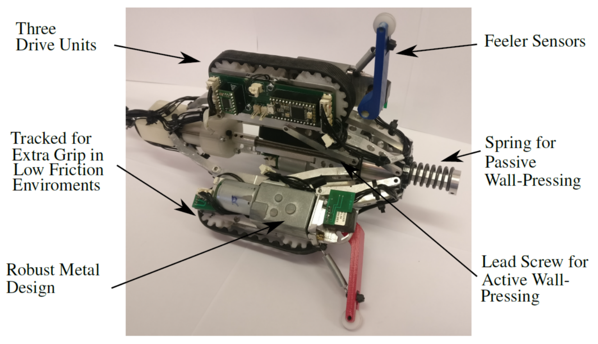
A Tracked, Differential-Drive, Wall-Pressing robot was developed for this task. It is the next prototype in the FURO line [3]. Figure 5 shows an annotated image of the prototype.
It features both active and passive wall-pressing via a central lead screw and spring assembly, it is able to change its diameter from 137.02 to 243.66 mm. This allows the robot to passively alter its diameter to fit through elbows as well as varying pipe diameters but is also able to drive the lead screw for greater changes in pipe diameter and to increase its wall pressing force. This allows the robot to navigate both horizontal and vertical sections of pipework. With the wall pressing providing more than sufficient force to stop the 1.99 kg robot slipping when climbing. The three motors have a maximum torque of 4.3 Nm which allows them to propel the robot in vertical sections of pipe.
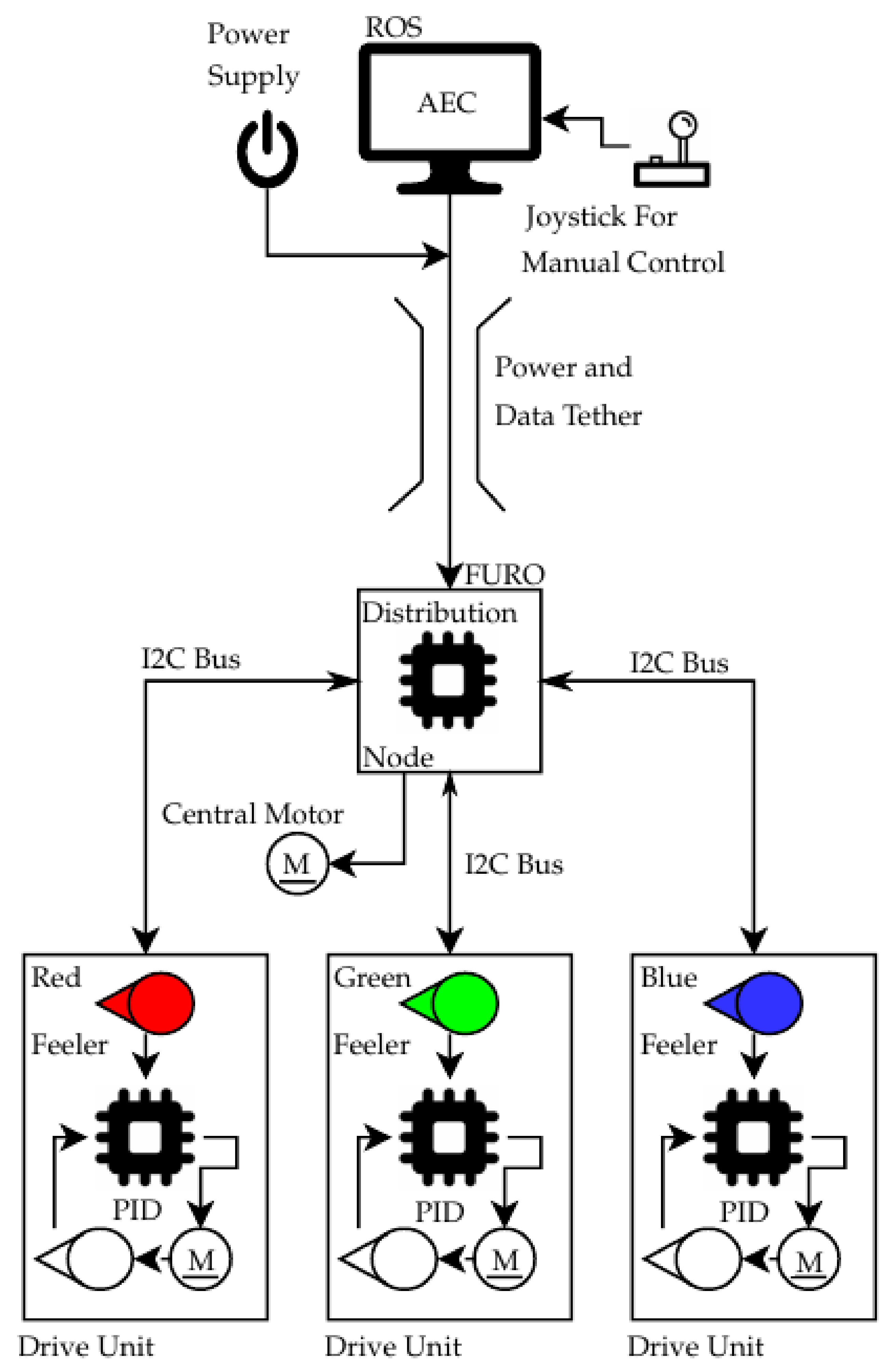
Each of the three DUs contain a worm geared motor which drives a rubber track for extra grip in low friction environments and they also contain a microcontroller. These controllers are responsible for running the low-level PID velocity control for each track using an encoder on the passive wheel as the input, and used for sampling their feeler sensor. Each DU microcontroller communicates to the distribution node over an I2C bus and this node interfaces with ROS and relays the set point and sensor information. In addition to this, it also controls the central wall pressing motor. The control architecture is shown in Figure 6. The chassis of the robot is constructed from aluminium as 3D printed parts were previously used which could not withstand the forces applied to the robot in the corners.
The overarching controller for the robot is implemented using the ROS framework [22]. This controller sends set points to the low level controllers on each DU and handles the commanded velocities from the AEC. The FURO II robot is presented in greater detail in [12].
- Feeler Sensor:
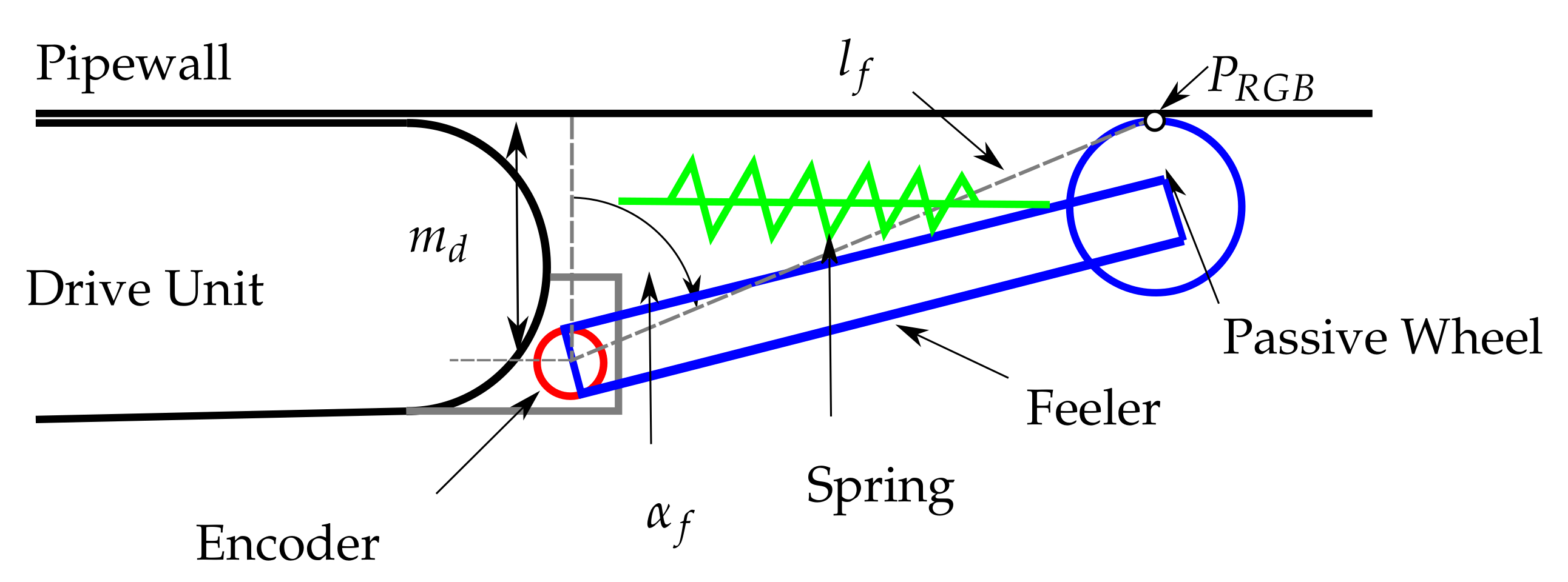
The sensor design consists of an arm that follows the pipe wall with a method of feeding back the angle. As the corner can change in any direction, a set of three feelers which are equally separated around the pipe are required, their separation is defined by . The feelers are mounted ahead of the robot to allow the estimation to be made before the robot enters the elbow. The feelers consist of an encoder to measure the angle, a passive wheel to reduce the contact friction and a spring to pull the feeler onto the pipe wall. The feeler sensors were developed in [3] which describes them in further detail.
The measured angle from the sensor is defined as . It is recorded as it travels along the pipe ahead of the robot. Figure 7 shows a simplified diagram of the design with the key parameters labelled. The mounting height (), feeler length (), feeler contact point (, note RGB is used to differentiate between the three feelers) are also shown. The real feeler sensors are mounted on the FURO II prototype in Figure 5.
In addition to the feeler, an on-board encoder is mounted on the passive wheel of the tracks. To simplify visualising the feeler data, the three sensors are referred to by colour—red, green and blue (RGB).
3. Autonomous Control Strategy
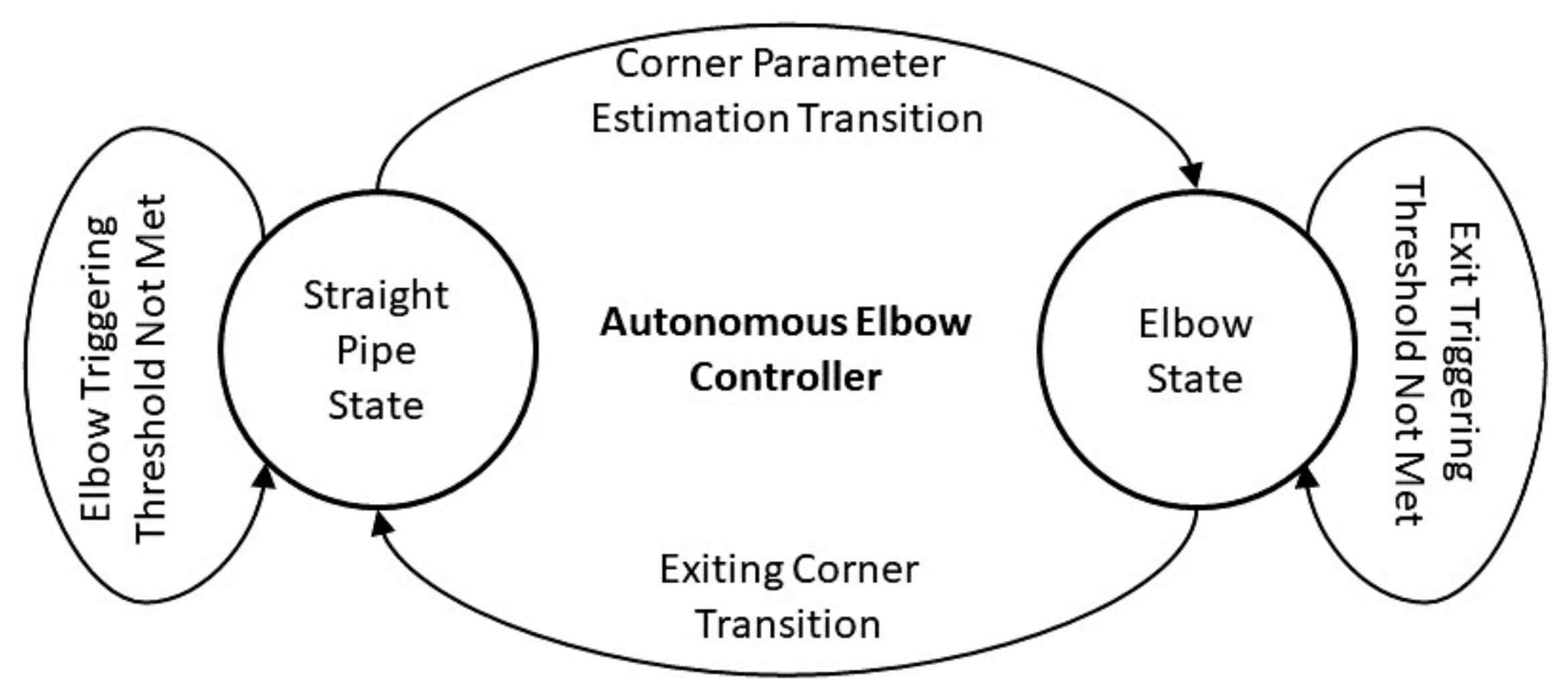
The proposed method has two main states of operation, the straight pipe state and the elbow state. The controller forms the basis of the transition into and out of the elbow state. Figure 8 shows the basic overview of this controller with the transitions labelled. This controller implement used ROS and is the highest level controller in the system. This is shown in Figure 6.
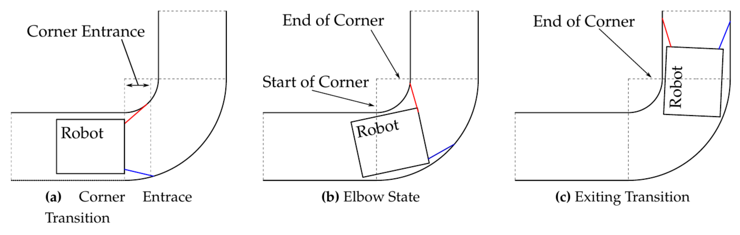
The representation of the states and transitions of the controller is shown in Figure 9. As the robot transitions from the straight pipe state to the elbow state (a). (b) The elbow state where the robot is traversing the corner. (c) The transition out of the elbow state to the straight pipe state.
Each of the transitions and states are described in further detail below.
3.1. Straight Pipe State
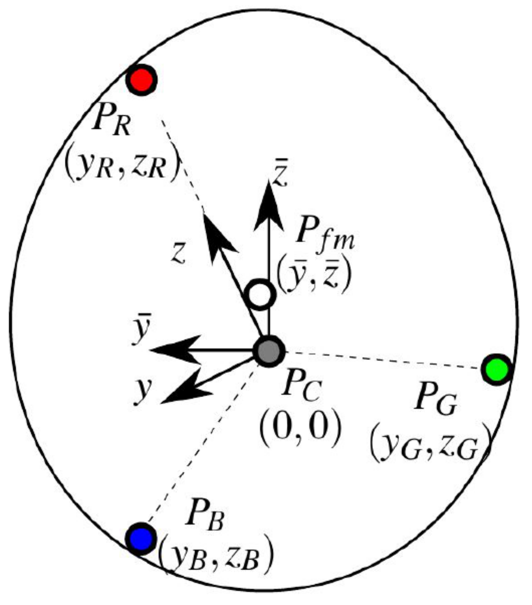
Operating in a straight pipe is the normal condition for the robot. When in this state, the DU velocities are all equal and no turning is taking place. The feeler sensors mounted on the front of the robot are being monitored for any change to determine if the robot is entering a junction. The parameter being monitored is the average position of the feeler end positions () given by
where , and are the three feeler coordinates, which are derived from their kinematic model [3] and shown in Figure 7 as . The combination of the end positions of the feelers is shown in Figure 10 where is the centre of the robot in the y–z axis and is the sum of the feeler end points (1). The distance between , and is given by
In the straight part of the pipe this distance is near zero, whereas it increases as the robot enters a corner. As a result, the distance in (2) is monitored to determine if the robot has entered an elbow. The threshold for this value was experimentally found to be 1 mm.
Once this triggering threshold is met, the corner parameter estimation transition from the straight pipe state to the elbow state begins.
3.2. Corner Parameter Estimation Transition
This transition is responsible for the change between the straight pipe and elbow states. During this transition, the controller is determining the parameters of the elbow such that it can generate the appropriate velocities to safely turn the elbow in the elbow state. The corner parameters are shown in Figure 4, the required parameters to determine the control action can all be estimated at the start of the corner, except the corner angle (). As is unknown, the proposed control method of sensing for exit conditions allows the AEC to work without it and navigate an elbow with any corner angle, this will be explained in greater detail in Section 3.3. The feeler sensors are used to estimate the corner direction () and can be used to determine major radius (R) as presented in [3]. Note that is the actual corner direction whereas is the estimated direction. Once the values are estimated the controller enters the elbow state.
3.3. Elbow State
The elbow state is responsible for traversing through the elbow. Using the estimation of the elbow parameters from the previous transition, the robot calculates and sets its DU velocities. The method of achieving this is presented in [3]. Once calculated, the set points are sent to the low level speed controllers for each DU on the robot. Once these are set, no other control actions are taken and the robot should progress around the elbow, as shown in Figure 9b. If there is any error in the estimation of the elbow parameters from the previous transition, the calculated velocities will also have an error. This error will show itself in the form of slip in the tracks.
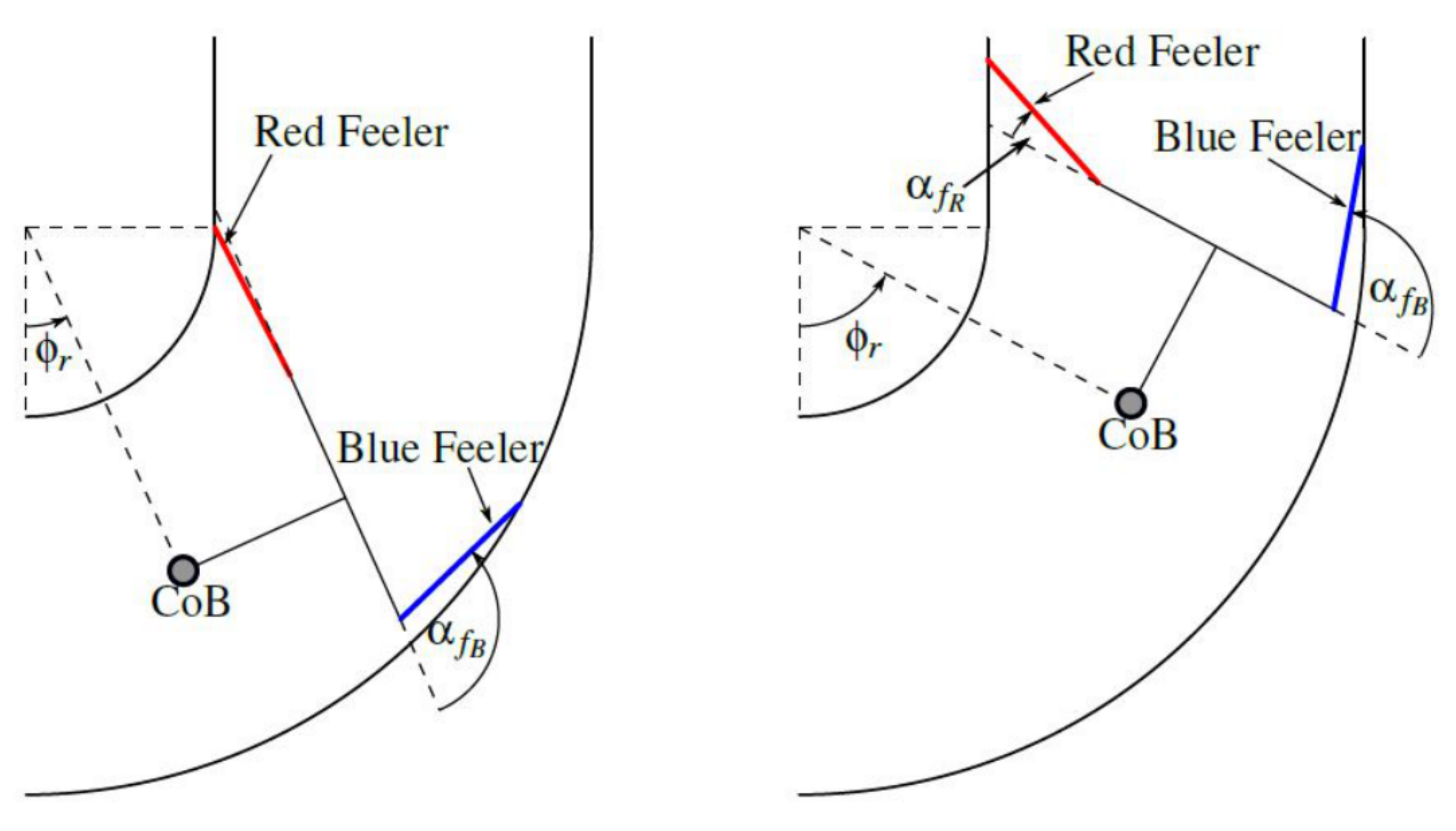
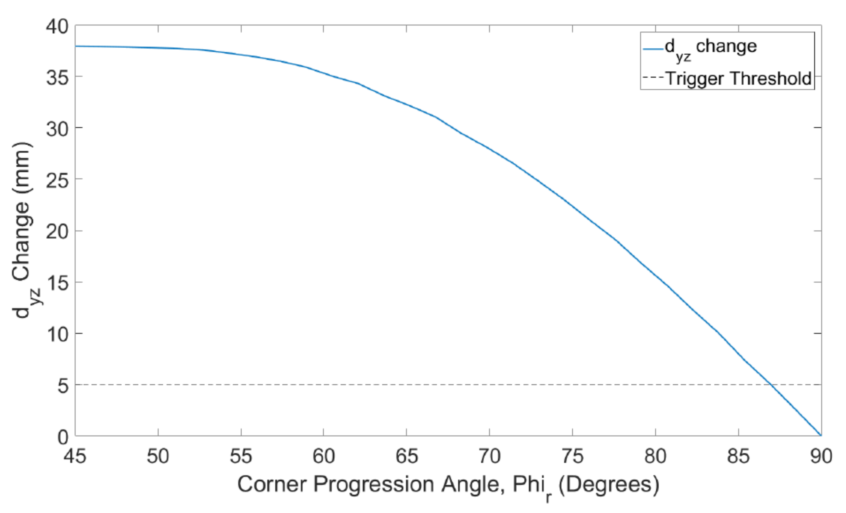
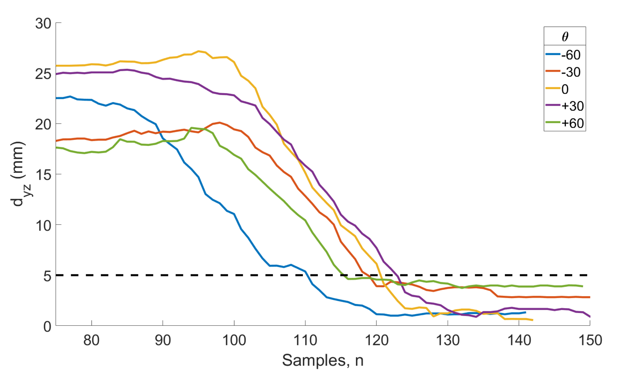
To leave the elbow state, the feeler sensors are used to detect when the robot is leaving the elbow. The conditions it is monitoring is the magnitude of change of the feelers, , to determine a threshold for triggering out of the elbow state a model is created to calculate the feeler angles and thus end position. The model determines the feeler angles () as the robot passes through the elbow, highlighted in Figure 11. The full details of the feeler angle estimation model are shown in Appendix A. The output of the model is shown in Figure 12 as the robot passes through the corner (with ). As would be expected, the magnitude of change of the combined feeler sensors () tends to zero as the robot enters the straight pipe and the feelers centre themselves. The value selected for this was found from experimentation and 5 mm is selected. This ensures the corner is exited and is sufficiently close to the final value to not cause major slipping in the end of the pipe. An extension to this work could explore the possibilities on the tuning of this value. A distance threshold is also set before the transition can be triggered, to overcome any defects in the corner which could artificially lower the value at the start of the turning stage.
As the controller is detecting for exit conditions, the corner angle () can be variable as the velocities for each DU are set based on the other parameters. The robot will keep turning the elbow until the exit transition is triggered.
Once the triggering threshold has been met the robot enters the exiting transition.
3.4. Exiting Transition
The exiting transition is triggered as the robot is leaving the elbow and transitioning back into the straight pipe state. This is shown in Figure 9c. This transition is very straight forward as the velocities for navigating in a straight pipe are already known (all equal); thus, no calculations have to be complete. In the transition, the velocities are set back to equal and the straight pipe state is then entered.
4. Experimental Hardware and Methodology
This section presents the hardware and methodology used for the validation of the AEC.
4.1. Pipe Network
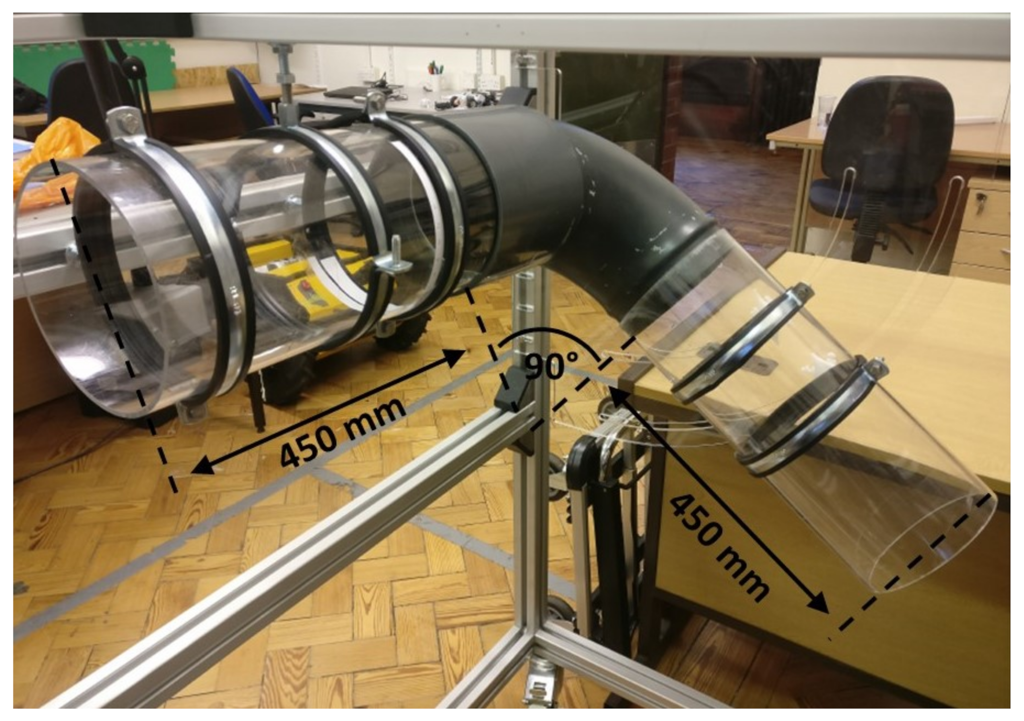
To test the proposed control method, an experimental rig is constructed. The test rig consists of two 450 mm long, 150 mm inside diameter sections of acrylic pipe joined with a short cast iron 90° elbow with the major and minor radius of mm. Due to the slight increase in diameter in the elbow and the slip on fittings, there is a small lip on the entrance and exit of the pipe. Due to its construction method, the elbow has a rough seam where the two halves were joined. It was selected due to availability of large diameter pipe elbows. Angle markers are placed on the outside of the 1st pipe section to align the robot for the tests, 0° aligned with the short path around the elbow. The rig is shown in Figure 13.
4.2. Experimental Procedure
The robot is aligned with angle markings on the section of pipe before the elbow in the pipe network and the autonomous control is started (either AEC or BF). While the robot passes around the corner, the feeler, encoder data and time are recorded. The experiment is run in 10° steps between and three passes are complete at each angle with AEC running. is selected as it gives a total range of 120°, as the robot consists of three drive units equally separated, it is symmetrical every 120° meaning angles are sufficient to encounter every unique entrance angle in relation to a drive unit. A smaller sample is taken using the BF method to reduce the damage on the FURO II robot. Both control methods have the same average velocity set point of 10 mms for following the transition of the elbow.
4.3. Comparison Metric: Impulse
Due to the reviewed methods in Section 1.3 providing limited or no metrics for their cornering methods, the system will be benchmarked and tested against the BF method. The literature will be included in the discussion of the practical experiments for comparison. The metric selected to review the system is Impulse (Ns).
Impulse (I), measured in Newton seconds, is used to determine the amount of extra force applied to the robot when its DUs are forced to slip in the corner and is given by
where is the time spent slipping (or slip time) and is the force required to make the tracks slip (the force required to overcome static friction). This Impulse can be used to identify the additional force being applied to the robot over a span of time; thus, the greater the Impulse the greater the force applied to a robot over a given time or the greater the time the force is applied to the robot. A larger or longer force applied to the robot is likely to cause damage to it. Therefore, the lower the Impulse the better.
This time () is the time the robot spends with any of its tracks or wheels slipping in the elbow. The slip itself occurs when there is a disparity between the estimated (or calculated) velocities and the real values. As the robot is a rigid body, it is not possible for the tracks to exit the corner at different times; thus, any disparity will cause one or more DUs to slip.
To determine the , it is assumed that the cornering time of the robot will be the same as the calculated slowest path, be that a fast track speed on a longer path or a slow track speed on a short path. The difference in the calculated path completion time between the multiple DUs is the slip time . Using this , the I can be determined once is known.
As is the force required to overcome static friction it must be greater than the normal force () being exerted by the robot’s spring mechanism and the coefficient of static friction (), i.e.,
Both and can be determined from the FURO II robot and type of pipe, N and . The coefficient of static friction () being used was found experimentally using the spring balance method with the tracks of FURO II and the materials of the test pipe network. Therefore, the force required to overcome the static friction is
Now that and are known, I can be calculated using (3).
5. Results and Discussion
This section presents the results from the experiment explained above. It is followed by a discussion on the outcomes of the tests and a comparison with the BF method.
5.1. Experimental Results
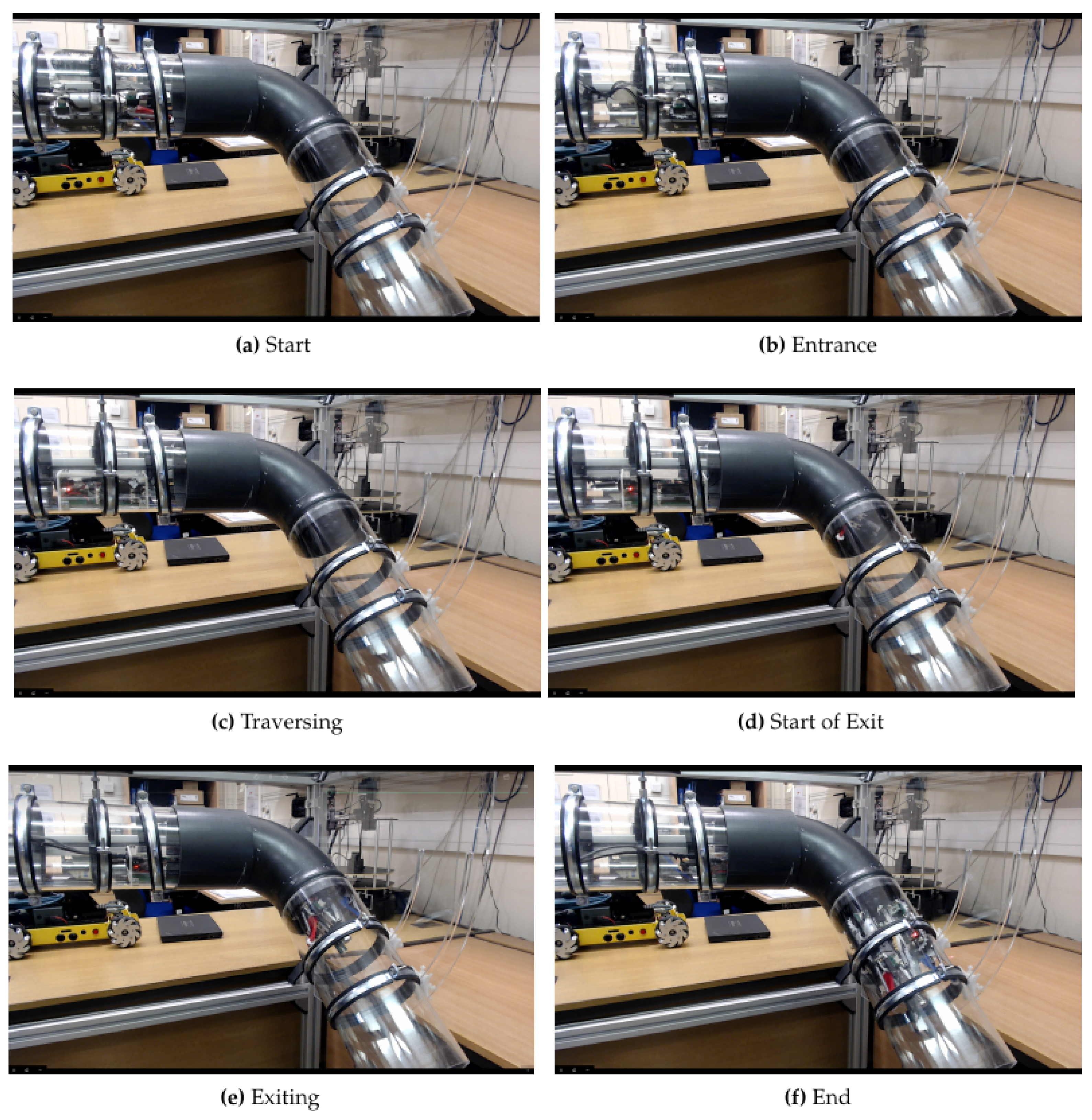
Figure 14 shows the robot passing through the corner, videos of the turning can be found at (https://www.youtube.com/watch?v=F-mmlID0mDA). The robot is placed at an entrance angle and is running on AEC. The robot is able to successfully pass through the elbow and comparing it to the BF method on average it has a reduction in the Impulse applied to the robot of 213.97 which is a major decrease. For all 39 repeats using AEC taken for the experiment, the robot was able to navigate the elbow successfully. Comparing this to BF which only completed four out of nine passes shows the effectiveness and requirement of the AEC controller. The results from the experiment are broken down into the three sections to allow a more detailed review of each stage.
5.1.1. Entering
The entrance stage of the controller is responsible for both the estimation of the corner direction as well as the calculation of drive unit velocities.
Due to misalignment of the angle marker with the actual corner direction, a systematic offset has been removed from the results. The estimate from the AEC testing is shown in Figure 15. It can be seen that the predicted angles are close to the true value. The mean absolute error in the prediction is which is a minor improvement over the results from [3].
5.1.2. Traversing
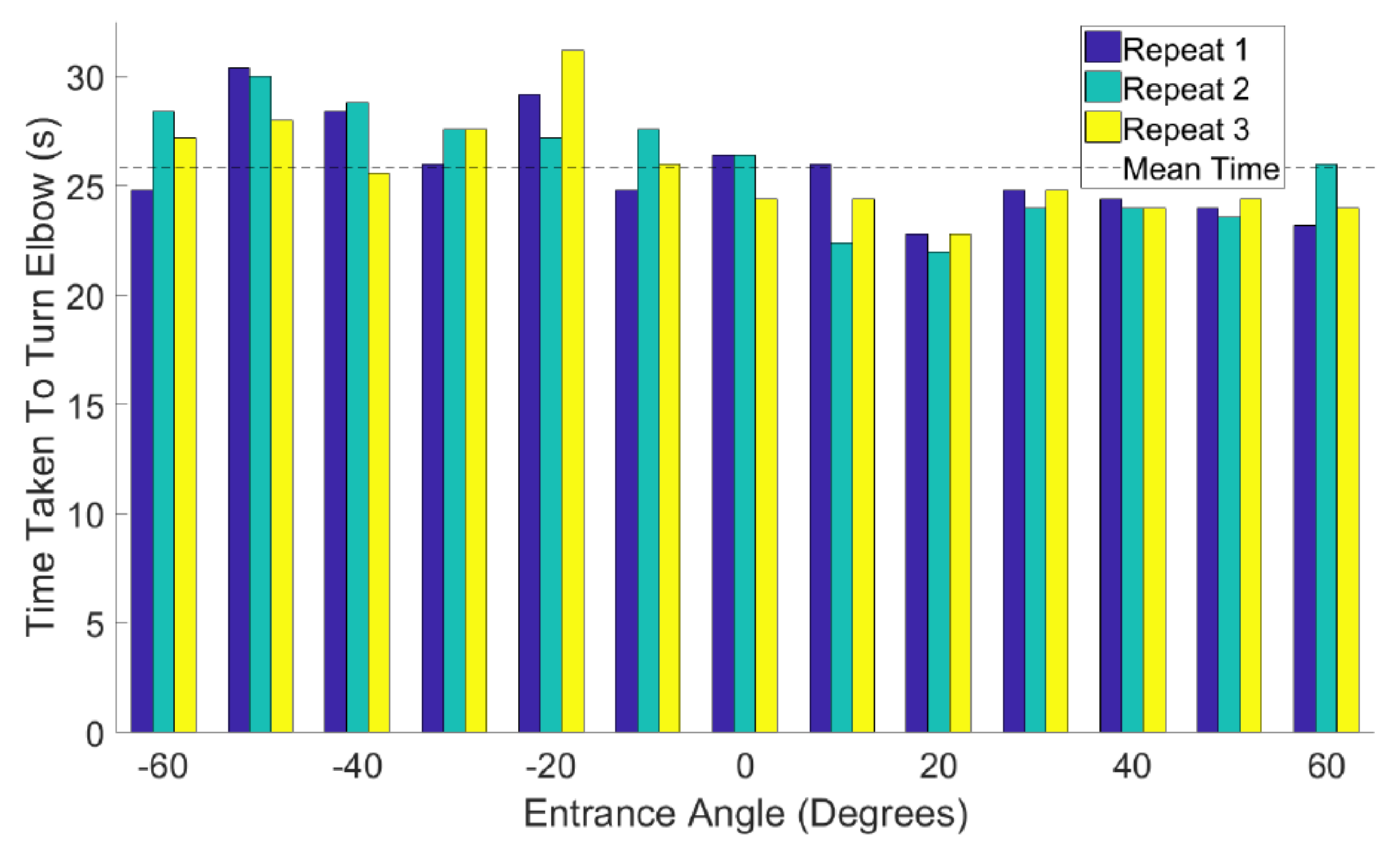
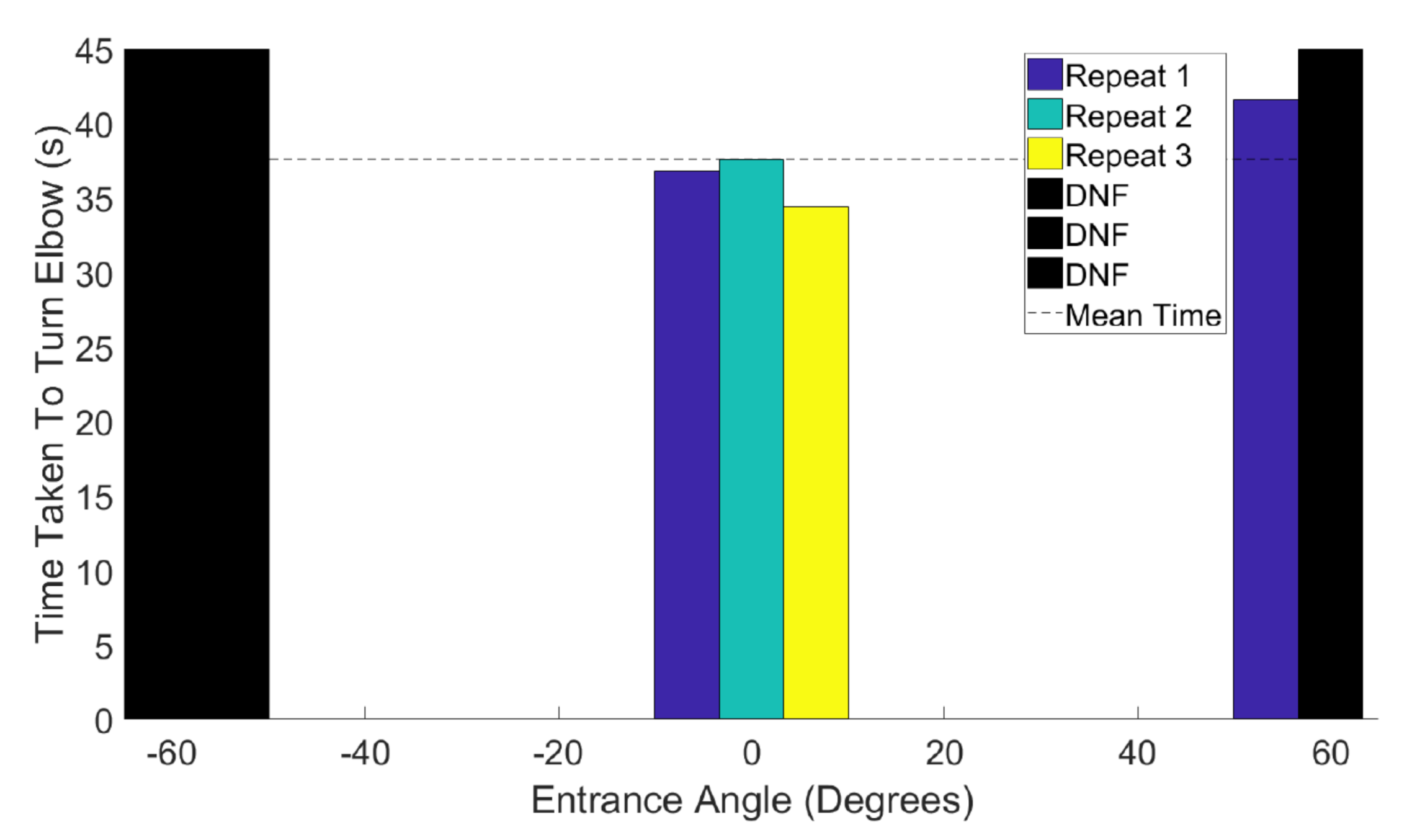
To review the traversing section, the time taken for each pass with the AEC is compared with BF. The time taken can be used to determine the Impulse applied to the robot using (3). Figure 16 shows a plot of the time taken for each pass using the AEC and Figure 17 for BF. The black bars show when the robot got lodged in the elbow, not completing the turn and receiving a Did Not Finish (DNF) label.
The time for each completed pass is shown in Figure 16 and Figure 17. There are very few passes using the BF method due to the damage the testing caused to the FURO II robot. After the ninth pass the robot was broken when completing the BF testing. When using the AEC, the robot not only completed all 39 passes but also had no damage done to the robot during them.
The average turning time using the AEC is s with a maximum s and minimum s. For the BF method, the average turning time is (if excluding the DNF results) with a minimum time of s and maximum of s.
Reviewing the four DNF passes, three of them occurred at and the final one at . The robot is symmetric at those two values where one DU is travelling along the longest path around the outside of the elbow and the other two are equidistant from shortest path. This would mean at the robot would have the most force pushing it in the opposite direction to the corner leading to it getting stuck.
An observed event which cannot be seen in the data sets that occurred during the BF testing was the robot skipping teeth on the tracks. This is due to the slipping required and in this case, the slipping occurred on the mating face between the drive cog and the track as opposed to the track on the pipe wall.
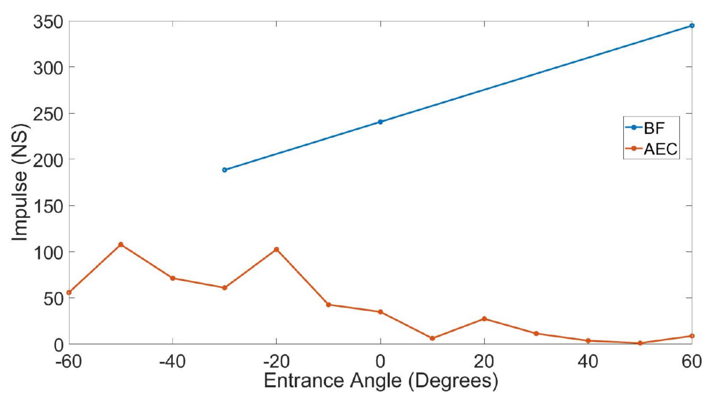
To review the data in terms of the Impulse metric, the turning time for each entrance angle has been averaged for both the BF (removing the DNF passes) and AEC methods. The Impulse applied to the robot is calculated using the method present in Section 4.3. The results are shown in Figure 18.
It can be seen in the figure that the impulse applied to the robot using the BF method is significantly greater than using the AEC, showing the advantages of the controller over that method. However, there is still Impulse applied to the robot when using the AEC, showing there is room for improvement on the estimation of the elbow parameters. Comparing the average turning time of the two methods, the mean time difference is s. This means, on average when using the BF method, the robot will slip for s more than if using the AEC method. Again, using Impulse, the average increase applied to FURO II in the elbow using the BF method gives Ns, which is a very large increase meaning there is much greater fatigue on the robot.
5.1.3. Exiting
The exit conditions are triggered by monitoring the value of combined with a distance threshold. The simulated change in Figure 12 shows all the values converging to zero as the robot exits the corner. The real data of five passes taken at , , 0, and are shown in Figure 19.
The change shown in the figure is for the end of the traversing and whole exit stage. The values plateau as the robot is in the traversing phase and start to drop down as the robot exits. The exit triggering threshold of mm is shown on the figure. All the changes drop below that value, and at that point the DU velocities are set to the straight section of pipe. Further work could be completed on tuning this value.
5.2. Discussion
Following the analysis, the results are discussed in more detail in the following section.
5.2.1. Entrance
The corner direction estimation is an improvement on the experimental values from [3], with a mean error of comparing to . This result is comparable to the related work by Choi et al. [23] and Kim et al. [24] with mean errors () of and , respectively, in their predictions over very limited recorded passes. Both their solutions required large sensors which would be unsuitable for small pipework and required large amounts of computation.
This shows that the feeler sensors offer a competitive, low-cost (both financially and computationally) and scalable method for estimating corner direction.
5.2.2. Traversing
During the traversing stage is where the major differences between the two methods are shown with their ability to turn the corner. The BF method caused the robot to get stuck in the corner on four of the nine passes through the elbow. It also broke the FURO II robot stopping further testing. Whereas, with the AEC, despite a small error in the estimation, it completed all 39 passes. This shows the advantages of the controller over the BF method.
Further analysis can be completed by looking at the turning time and Impulse between the two methods. The average increase in time between BF and the AEC is s. This is a significant amount of time when the target turning time is s. The increased time taken by the BF method translates to the extra Impulse exerted on the robot of Ns. This is a significant increase over the controlled method showing there is a large improvement when using the AEC.
Comparing the AEC time of s to the target time shows that there is a small difference. This could be due to errors in the prediction. Despite the slight increase from the target time (), the improvement compared to the BF method is clear.
5.2.3. Exit
Looking at the change in from Figure 19, the threshold value of 5 mm was suitable to trigger the exit condition and allow the robot to leave the pipe. The final values for each pass are given when the robot is fully in the straight section of pipe. Despite the simulated values returning to zero, in the real results none of them achieve this, with the highest settling around mm. This is due to the robot becoming slightly twisted within the pipe which moves the mounting positions of the feeler sensors. This is caused by slight mismatches in speed of the DUs from errors in the estimation when traversing the corner, as well as minor manufacturing tolerances in the pivoting legs of the robot which allow it to move in undesirable ways. This could be addressed in software by resetting the feeler angle when the robot is known to be in a straight section of pipe or manufacturing the robot to tighter tolerances.
5.3. Comparison with Literature
There are very limited metrics used by the current methods of control within a corner, therefore they can only be compared on their success of cornering. The FURO II was able to complete 39 passes through the elbow using the AEC, MRINSPECT V has results of it navigating a pipeline with two elbows and a T-Junction and the IPR-D300 [11] completed an elbow but this caused a track to derail.
It can be seen that the AEC system on the FURO II prototype has been robustly tested in comparison to the literature and has a comparable performance but with the advantages of offering a scaleable and low-cost detection method that is suitable for any angle of elbow.
5.4. Scalability
The method of determining the parameters of a corner will work in both smaller and larger sized pipes than the demonstrated 150 mm. Increasing the pipe size would reduce the change in . At a very large increase the AEC would not be triggered as it would be less than the threshold value. In this case, longer feelers could be used on the robot to travel further into the elbow and thus see a greater change in . Smaller pipes would lead to a greater change to the for the same sized feeler sensors, to a maximum where the feeler arms would foul on the inside of the pipe rather than progressing through the elbow. Again, altering the length of the feeler sensors would remove this issue. The minimum standard diameter of pipe the sensor could operate in is 50 mm at which point off the shelf encoders could not be used and specially designed units would need to be made which would drastically increase the sensors cost. There is no foreseeable upper limit; however, in very large diameter pipes which would require very long feelers, the structural rigidity of the design would become very important which may mean they require major modification. In both cases, an estimation of the pipe diameter would be required to accurately calculate the DU velocities which could be built into a WP robot’s actuation mechanism.
5.5. Alternative Obstacles
5.5.1. Sharp Elbows and T-Junctions
Due to the set up of the feelers, they would be unable to navigate past T-junctions as the spring would pull the sensor into the branch causing the robot to become caught if it proceeded further. A method of retracting the feeler sensors would be required to enable the robot to pass this obstacle. A Sharp elbow is a 90° bend with a major radius of . These could be detected by the sensors and would give a direction estimation, however as the radius of the elbow would be much tighter the calculated velocities would be inaccurate. To overcome this, a case would need to be added to the controller which would identify the increased change and compensate accordingly.
5.5.2. Pipe Diameter Change
The sensors and robot would be able to overcome both an increase and decrease in pipe diameter unless the decrease was stepped which would cause the feelers to get trapped. The change in the pipe diameter would be detected by the feelers but as the sum of the relative change () would be zero the AEC would not be triggered. An additional case could be added to the controller to detect this event occurring and allow the robot to alter its diameter accordingly. Based on the current FURO II design, the minimum and maximum diameters it can operate in are 137.02 mm and 243.66 mm, respectively.
6. Summary and Contribution
This paper presents a novel AEC which utilises low-cost feeler sensors to safely navigate a pipe elbow with an unknown direction and angle. From practical experimentation, the AEC method allowed the robot to pass through the corner on every attempt (39 in total) whereas the BF method got lodged in the elbow four out of the nine passes it tried. This clearly shows the advantage and requirement for the AEC over the BF method. Comparing the Impulse applied to the robot, the AEC yielded a decrease of Ns compared to BF. The method is currently limited to short elbows and the feeler sensors would get caught when approaching different obstacles but this can be addressed with future work. The final results were comparable to the current state-of-the-art and the advantages of this method of control are that it only requires the use of three low-cost feeler sensors and is applicable to a large range of pipework sizes.
Further Work
Further work on using the FURO II prototype will be extending the estimation to determine the elbow major radius. This would allow the AEC to safely navigate around a greater variety of elbows and different radii of elbows. As discussed in Section 5.5, the development of a method to retract the feelers would be desirable to allow additional obstacles to be overcome.
Author Contributions
L.B.; methodology, software, formal analysis, investigation, data curation, writing, visualization. J.C. and S.W.; Conceptualization, supervision, writing—review and editing. All authors have read and agreed to the published version of the manuscript.
Funding
This project is supported by the Engineering and Physical Science Research Council (EPSRC) Project Ref: 1636964 and Sellafield Ltd.
Institutional Review Board Statement
Not applicable.
Informed Consent Statement
Not applicable.
Data Availability Statement
Not applicable.
Conflicts of Interest
The authors declare no conflict of interest.
Appendix A
Pipe Standards
The UK Health and Safety Executive (HSE) guide on the ‘Use of Pipeline Standards and Good Practice Guidance’ [25], follows the British Standard PD series of pipeline standards or the European standards implemented in the UK as British Normative Standards (BS EN series). Specifically, the ‘Onshore Major Accident Hazard Pipelines-BS PD 8010 Part 1’ within the BS EN standards. It should be noted that these standards are for steel pipeline, which is likely the material used in the majority of the pipework but the exact materials are unknown. As various materials for pipework are used in construction, such as plastics and other metals like cast iron, these standards will be taken as a general set of rules for the industrial pipework in the facilities this work is exploring.
Feeler Angle Estimation Model
This section describes the model used to estimated the feeler angles of the robot as it passes through an elbow, and this determines the change in magnitude of the combined feeler sensors ().
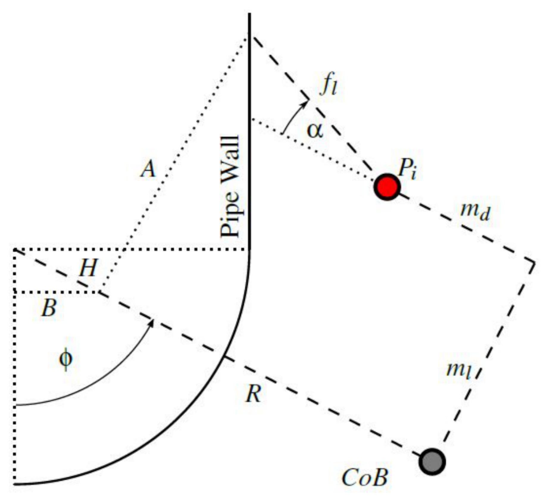
For the model, the parameters of the robot are taken from the FURO II prototype presented in Section 2, and the corner parameters are taken from the standard short pipe elbow for a 150 mm diameter pipe. A simulation can be made which generates the path of the feelers as the robot passes through the elbow using a model of the robot in an elbow, which determines the contact point on the inside of the pipe to find the angles of the feelers. A 2D simplified diagram of this is shown in Figure 11. It can be seen from the figure that as the robot progresses around the corner the feeler angles change. A more detailed view of the model can be seen in Figure A1, which shows the simulated robot exiting the elbow.
Figure A1.
Model of the robot exiting the elbow.

From Figure A1, R is the major radius of the pipe and is known or estimated in the entrance stage, is the length between the Centre of Body (CoB) of the robot to the feeler mounting point, is the height from the feeler mounting point to the centre of the robot and is the length of the feelers. All these variables (except R) are determined by the design of the robot.
To determine the feeler end position, the following intermediate variables are found
where is the rotation of the robot within the pipe. Then, the feeler end positions are given by
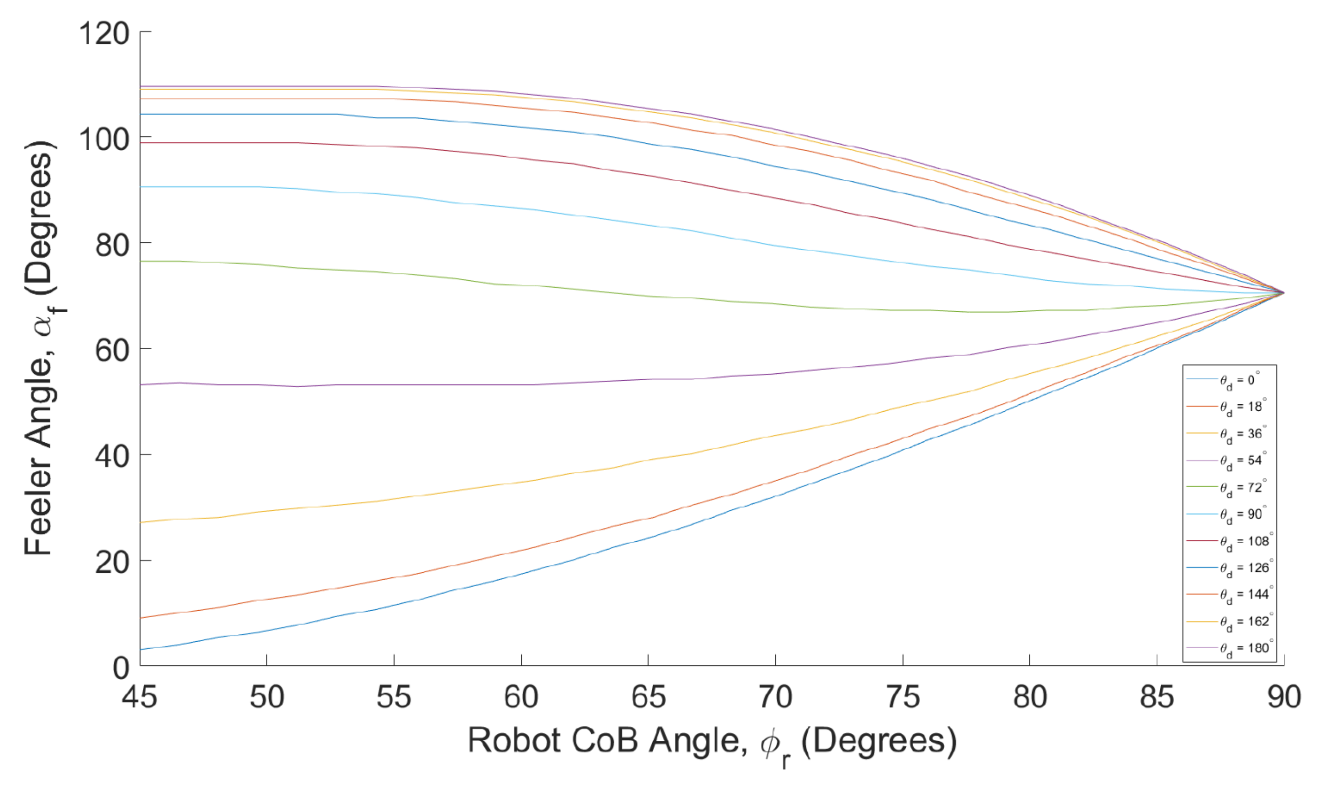
Using the model, the feeler angles can be found as it progresses through the corner. They can be seen in Figure A2.
Figure A2.
Feeler angles of exit conditions.

Note that Figure A2 shows only 10 offset angles (in the range 0° to 180°) of rotation, . As the robot progresses further into the corner and the feelers transition from the curved elbow to the straight section of pipe, the feeler angles all converge to their normal condition, i.e., when the feeler angle is at (this is defined by the design of the feeler sensor).
References
- Gov.uk. Nuclear Provision: The Cost of Cleaning Up Britain’s Historic Nuclear Sites-GOV.UK. Available online: https://www.gov.uk/government/publications/nuclear-provision-explaining-the-cost-of-cleaning-up-britains-nuclear-legacy/nuclear-provision-explaining-the-cost-of-cleaning-up-britains-nuclear-legacy (accessed on 9 January 2019).
- GameChangers. Post Operational Clean Out (POCO). Available online: https://www.gamechangers.technology/challenges/post-operational-clean-out-poco/ (accessed on 7 April 2020).
- Brown, L.; Carrasco, J.; Watson, S.; Lennox, B. Elbow Detection in Pipes for Autonomous Navigation of Inspection Robots. J. Intell. Robot. Syst. 2018, 1–15. [Google Scholar] [CrossRef] [Green Version]
- GameChangers. Identifying Unknown Sharps in Gloveboxes-Game Changers-Supporting Sellafield’s Nuclear Decommissioning Programme. Available online: https://www.gamechangers.technology/challenges/gloveboxes/ (accessed on 3 April 2020).
- EurekaMagazine. EurekaMagazine. The Vast Task of Decommissioning the UK’S Nuclear Facilities Is Driving and Rewarding Technological Innovation. Available online: https://www.eurekamagazine.co.uk/design-engineering-features/technology/the-vast-task-of-decommissioning-the-uks-nuclear-facilities-is-driving-and-rewarding-technological-innovation/182949/ (accessed on 11 September 2018).
- Roh, S.G.; Choi, H.R. Differential-drive in-pipe robot for moving inside urban gas pipelines. IEEE Trans. Robot. 2005, 21, 1–17. [Google Scholar]
- Rollinson, D.; Choset, H. Pipe Network Locomotion with a Snake Robot. J. Field Robot. 2016, 33, 322–336. [Google Scholar] [CrossRef]
- Okada, T.; Sanemori, T. MOGRER: A vehicle study and realization for in-pipe inspection tasks. Robot. Autom. IEEE J. 1987, 3, 573–582. [Google Scholar] [CrossRef]
- Okada, T.; Kanade, T. A three-wheeled self-adjusting vehicle in a pipe, FERRET-1. Int. J. Robot. Res. 1987, 6, 60–75. [Google Scholar] [CrossRef]
- Kim, J.H. Sensor-Based Autonomous Pipeline Monitoring Robotic System. Ph.D. Thesis, Louisiana State University, Baton Rouge, LA, USA, 2011. [Google Scholar]
- Zainal Abidin, A.S.; Chie, S.C.; Zaini, M.H.; Mohd Pauzi, M.F.A.; Sadini, M.M.; Mohamaddan, S.; Jamali, A.; Muslimen, R.; Ashari, M.F.; Jamaludin, M.S. Development of In-Pipe Robot D300: Cornering Mechanism. MATEC Web Conf. 2017, 87, 02029. [Google Scholar] [CrossRef] [Green Version]
- Brown, L. Autonomous Navigation of Unknown Pipe Networks; Technical Report; The Unviersity of Manchester: Manchester, UK, 2019. [Google Scholar]
- Nagase, J.Y.; Fukunaga, F. Development of a novel crawler mechanism for pipe inspection. In Proceedings of the 2016 42nd Annual Conference of the IEEE Industrial Electronics Society (IECON), Florence, Italy, 23–26 October 2016; pp. 5873–5878. [Google Scholar] [CrossRef]
- Lee, Y.G.; Kim, H.M.; Choi, Y.S.; Jang, H.; Choi, H.R. Control strategy of in-pipe robot passing through elbow. In Proceedings of the 2016 13th International Conference on Ubiquitous Robots and Ambient Intelligence (URAI), Xi’an, China, 19–22 August 2016; pp. 442–443. [Google Scholar] [CrossRef]
- Li, Q.; Sun, Y.; Liu, H.; Zhang, M.; Meng, X. Development of an In-Pipe Robot with a Novel Differential Mechanism; Springer: Singapore, 2018; pp. 1079–1097. [Google Scholar] [CrossRef]
- Kim, H.M.; Choi, Y.S.; Lee, Y.G.; Choi, H.R. Novel Mechanism for In-Pipe Robot Based on a Multiaxial Differential Gear Mechanism. IEEE/ASME Trans. Mechatron. 2017, 22, 227–235. [Google Scholar] [CrossRef]
- Zhang, Z.; Meng, G.; Sun, P. Kinematic modeling and simulation of wheeled pipe robot in elbow at planar motion stage. In Proceedings of the 2017 2nd Asia-Pacific Conference on Intelligent Robot Systems (ACIRS), Wuhan, China, 16–19 June 2017; pp. 227–233. [Google Scholar] [CrossRef]
- Chen, J.; Cao, X.; Deng, Z. Kinematic analysis of pipe robot in elbow based on virtual prototype technology. In Proceedings of the 2015 IEEE International Conference on Robotics and Biomimetics (ROBIO), Zhuhai, China, 6–9 December 2015; pp. 2229–2234. [Google Scholar] [CrossRef]
- Zhang, L.; Wang, X. Stable motion analysis and verification of a radial adjustable pipeline robot. In Proceedings of the 2016 IEEE International Conference on Robotics and Biomimetics (ROBIO), Qingdao, China, 3–7 December 2016; pp. 1023–1028. [Google Scholar]
- Lee, J.S.; Roh, S.G.; Moon, H.; Choi, H.R. In-pipe robot navigation based on the landmark recognition system using shadow images. In Proceedings of the IEEE International Conference on Robotics and Automation, ICRA’09, Kobe, Japan, 12–17 May 2009; pp. 1857–1862. [Google Scholar]
- Lee, C.H.; Joo, D.; Kim, G.H.; Kim, B.S.; Lee, G.H.; Lee, S.G. Elbow detection for localization of a mobile robot inside pipeline using laser pointers. In Proceedings of the 2013 10th International Conference on Ubiquitous Robots and Ambient Intelligence, URAI 2013, Jeju, Korea, 30 October–2 November 2013; pp. 71–75. [Google Scholar] [CrossRef]
- Quigley, M.; Faust, J.; Foote, T.; Leibs, J. ROS: An Open-Source Robot Operating System. Available online: willowgarage.com (accessed on 10 May 2018).
- Choi, Y.S.; Kim, H.M.; Mun, H.M.; Lee, Y.G.; Choi, H.R. Recognition of pipeline geometry by using monocular camera and PSD sensors. Intell. Serv. Robot. 2017, 10, 213–227. [Google Scholar] [CrossRef]
- Kim, S.H.; Lee, S.J.; Kim, S.W. Weaving Laser Vision System for Navigation of Mobile Robots in Pipeline Structures. IEEE Sens. J. 2018. [Google Scholar] [CrossRef]
- Health and Safety Executive. Use of Pipeline Standards and Good Practice Guidance. Available online: https://www.hse.gov.uk/pipelines/resources/pipelinestandards.htm (accessed on 29 January 2021).
Figure 1.
Photo of pipework from an exemplar facility.

Figure 2.
Short and long elbows.

Figure 3.
Pipe vehicle categories, based on [6].
Figure 3.
Pipe vehicle categories, based on [6].

Figure 4.
Elbow drive unit paths.

Figure 5.
FURO II prototype.

Figure 6.
FURO II control architecture.

Figure 7.
Simplified diagram of a feeler, modified from [3].
Figure 7.
Simplified diagram of a feeler, modified from [3].

Figure 8.
Autonomous Elbow Controller overview.

Figure 9.
Simplified diagram of Autonomous Elbow Control stages.

Figure 10.
Combining feeler end positions (in corner entrance).

Figure 11.
2D simplified diagram of exit conditions.

Figure 12.
Change in as the robot exits the corner.

Figure 13.
Test rig for experiments.

Figure 14.
FUROII prototype navigating the corner at entrance angle .

Figure 15.
Estimation of direction during Autonomous Elbow Controller testing.

Figure 16.
Time taken to turn using Autonomous Elbow Controller.

Figure 17.
Time taken to turn using brute force.

Figure 18.
Impulse applied to the robot while turning through an elbow.

Figure 19.
Real change in when navigating the elbow.


Table 1.
Robots and their cornering methods.
| Robot | Locomotion | Corning Method | |
|---|---|---|---|
| Nagase and Fukunaga | [13] | Tracked, WP | Compliant Design with BF |
| NIRVANA | [15] | Wheeled, WP | Multi-axis gear |
| MRINSPECT VII | [16] | Wheeled, WP | Multi-axis gear |
| Lee et al. | [14] | Wheeled, WP | Double Actuated Joint with BF |
| FAMPER | [10] | Tracked, WP | DD using Pre-determined map |
Publisher’s Note: MDPI stays neutral with regard to jurisdictional claims in published maps and institutional affiliations. |
© 2021 by the authors. Licensee MDPI, Basel, Switzerland. This article is an open access article distributed under the terms and conditions of the Creative Commons Attribution (CC BY) license (http://creativecommons.org/licenses/by/4.0/).
Share and Cite
MDPI and ACS Style
Brown, L.; Carrasco, J.; Watson, S. Autonomous Elbow Controller for Differential Drive In-Pipe Robots. Robotics 2021, 10, 28. https://0-doi-org.brum.beds.ac.uk/10.3390/robotics10010028
AMA Style
Brown L, Carrasco J, Watson S. Autonomous Elbow Controller for Differential Drive In-Pipe Robots. Robotics. 2021; 10(1):28. https://0-doi-org.brum.beds.ac.uk/10.3390/robotics10010028
Chicago/Turabian StyleBrown, Liam, Joaquin Carrasco, and Simon Watson. 2021. "Autonomous Elbow Controller for Differential Drive In-Pipe Robots" Robotics 10, no. 1: 28. https://0-doi-org.brum.beds.ac.uk/10.3390/robotics10010028
Note that from the first issue of 2016, this journal uses article numbers instead of page numbers. See further details here.