Dynamic Parameter Identification of a Pointing Mechanism Considering the Joint Clearance

Abstract

The clearance of the revolute joint influences the accuracy of dynamic parameter identification. In order to address this problem, a method for dynamic parameter identification of an X–Y pointing mechanism while considering the clearance of the revolute joint is proposed in this paper. Firstly, the nonlinear dynamic model of the pointing mechanism was established based on a modified contact model, which took the effect of the asperity of contact surface on joint clearance into consideration. Secondly, with the aim of achieving the anti-interference incentive trajectory, the trajectory was optimized according to the condition number of the observation matrix and the driving functions of activate joints that could be obtained. Thirdly, dynamic simulation was conducted through Adams software, and clearance was involved in the simulation model. Finally, the dynamic parameter identification of the pointing mechanism was conducted based on an artificial bee colony (ABC) algorithm. The identification result that considered joint clearance was compared with that which did not consider joint clearance. The results showed that the accuracy of the dynamic parameter identification was improved when the clearance was taken into consideration. This study provides a theoretical basis for the improvement of dynamic parameter identification accuracy.

1. Introduction

With the development of industrial robots, the requirements for robot performance have increased [1,2]. In the traditional position control of robots, it is difficult to achieve a high performance and adapt to complex working environments. A control strategy based on a dynamic model is an effective method to improve kinematic accuracy and reliability [3]. An accurate dynamic model and dynamic parameters comprise the foundation of high-precision control [4]. The accurate identification of the dynamic parameters, which appear in equations that define the dynamic behavior of a robotic system, is essential for both the implementation of advanced control schemes and the dynamic simulation of such mechanical systems.

The methods for solving dynamic parameters include: disassembly measurement, the Computer Aided Design (CAD) method, and overall identification. Compared with other methods, overall identification has many advantages, and current dynamic parameter identification mostly adopts this method [5,6]. The standard process of dynamic parameter identification includes dynamic modeling, excitation trajectory design, data acquisition, and parameter identification [7,8]. The methods for establishing a rigid body dynamic model of a robot mainly include the Newton–Euler method, the Lagrange method, and the virtual work principle method [9]. Atkeson used the Newton–Euler method to establish the dynamic model of a Programmable Universal Manipulation Arm (PUMA) 600 robot [10]. Based on the virtual work principle, Huo et al. established the dynamic model of a 2-degree-of-freedom (DOF) tracking mechanism [11]. To carry out dynamic parameter identification, excitation trajectory is necessary. Excitation trajectory is usually divided into two parts: trajectory model selection and trajectory parameter optimization. The trajectory should have good periodicity and a sufficiency of excitation [12]. Swevers et al. suggested using the finite Fourier series function to guarantee periodic excitation [13]. In order to improve noise immunity performance, the trajectory must be optimized [14]. Armstrong proposed the use of the condition number of an observation matrix for the optimization of the excitation trajectory [15]. The issue of dynamic parameter identification is usually transformed into the optimization of a multi-dimensional nonlinear function, which takes the deviation between the dynamic model and experimental data as the objective function [16]. Park used the least square method to identify the dynamic parameters of an industrial robot [17]. Gautier et al. proposed using the least squares estimation method and an extended Kalman filter for robot dynamic parameter identification [18,19]. However, the least square method is extremely sensitive to noise [20]. To overcome this problem, data filtering can be adopted to improve the noise immunity [21]. A genetic algorithm can be used for dynamic parameter identification as well, but its convergence rate is slow [22]. Ding et al. developed a chaotic artificial bee colony (ABC) algorithm to avoid the problem of local optimization and carried out the identification of a 6-DOF industrial robot and a small-scale helicopter [23,24]. The artificial bee colony algorithm, which has significant advantages in nonlinear function optimization, can be used well in dynamic parameter identification [25,26].

Due to manufacturing tolerances, material deformation, and motion requirements, the clearance of a revolute joint is inevitable [27]. Schwab et al. used an impact model and a Hertzian contact force model to predict the dynamic response of mechanisms with joint clearance [28]. Joint clearance can bring violent collisions and affect dynamic performance of the mechanical system [29,30]. A larger clearance size corresponds to a higher contact force in a clearance joint [31]. Erkaya investigated the effects of joint clearance in a robotic system and used a neural model to predict the trajectory deviations from the working process [32]. Flores et al. presented and discussed a comprehensive combined numerical and experimental study on the dynamic response of a slider-crank mechanism with revolute clearance joints [33]. The Kriging mathematical model was used for dynamics of mechanical systems with revolute joint clearances, which can predict the dynamic performance efficiently and allow for the visualization of the trends of the response surfaces when the design variables are changed [34]. Li et al. developed the dynamic model of a Delta robot with joint clearance and used a Kriging-based model to calculate clearance value [35]. Ruderman et al. identified backlash by mounting a high-precision encoder on the joint side [36]. Erkaya et al. used Genetic Algorithm (GA) to implement the optimization of link parameters for minimizing the error between desired and actual paths due to clearance [37].

Because joint clearance affects dynamic response, including the torque of revolute joint. When the dynamic model without considering the joint clearance is used for dynamic identification, the effect of the joint clearance on joint torque is ignored and the dynamic parameter identification accuracy is reduced. A lot of research work on dynamic parameter identification has been done. Many researchers studied the effects of clearance on dynamics of mechanical systems and made efforts to reduce the influence of clearance. However, the effect of revolute joint clearance on the dynamic parameter identification accuracy is ignored currently. The accurate dynamic parameters, especially inertial parameters, are important to high-performance control. When the dynamic model considering the clearance is used for dynamic parameter identification, it is beneficial to the improvement of the identification accuracy. It is meaningful for high-performance dynamic control. Therefore, this paper proposes using the dynamic model considering revolute joint clearance to conduct the dynamic parameter identification of a X–Y pointing mechanism. In addition, the asperity of contact surface is taken into consideration to modify the contact stiffness and damping coefficient, which is beneficial to the improvement of the dynamic model accuracy.

Based on the fractal theory, the Newton–Euler approach, and the ABC algorithm, a method for dynamic parameter identification of an X–Y pointing mechanism while considering the clearance of the revolute joint is proposed in this paper. The results of the identification that considered joint clearance was compared to identification that did not consider joint clearance. The rest of this paper is organized as follows. Section 2 describes the nonlinear dynamic model of the pointing mechanism. Excitation trajectory optimization is discussed in Section 3. Parameter identification and simulation analysis are discussed in Section 4. Finally, Section 5 concludes the paper.

2. Nonlinear Dynamic Model of the Pointing Mechanism

The process of establishing a dynamic model includes a normal contact force model, a description of clearance, a friction model, and a dynamic modeling method. In order to make a dynamic model more accurate, a normal contact model takes the asperities of contact surface into consideration based on fractal theory. Here, the coefficients of contact stiffness and damping in the Lankarani–Nikravesh (L–N) normal contact force model were modified. Modified Coulomb friction model was chosen as the friction model. The dynamic model of the pointing mechanism was established by the Newton–Euler approach.

2.1. Normal Contact Force Model

A contact model is a critical issue of a dynamic model when clearance and asperities are taken into consideration. The L–N nonlinear spring damping model is widely used for analyzing contact and collision issues. However, the asperities of contact surface are not taken into consideration in the L–N model, which can influence the normal contact stiffness and damping. In order to make the normal contact model more accurate, a modified L–N model, which was proposed in our previous research work, was chosen as the normal contact model [38].

Based on the Majumdar–Bhushan (M–B) fractal theory [39], the distribution function $n(a^{\prime })$ and the real contact area $A_r$ of the asperities on the contact surface of the moving pair can be expressed as:

$$\{\begin{array}{l}n\left(a^{\prime }\right)=\frac{D-1}{2}{\phi }^{\left(3-D\right)/2}\frac{a_l^{\prime }{}^{\left(D-1\right)/2}}{{a^{\prime }}^{\left(D+1\right)/2}}\left(2<D<3\right)\\ {\phi }^{\left(3-D\right)/2}-{\left(1+{\phi }^{-\left(D-1\right)/2}\right)}^{\left(D-3\right)/\left(D-1\right)}=\frac{3-D}{D-1}\left(2<D<3\right)\\ A_r=\frac{D-1}{3-D}{\phi }^{\left(3-D\right)/2}{a}_l^{\prime }\end{array}$$

(1)

where $a^{\prime }$ is the contact area of asperities, $a_l^{\prime }$ is the maximum contact area of asperities, D is the fractal dimension, $D=\frac{1.54}{R_a{}^{0.045}}+1$, and φ is the domain extension factor of the contact asperity size distribution [40].

The critical compression depth and critical contact area of the asperities in elastic deformation are expressed as:

$$\{\begin{array}{l}{\omega }_c={\left(\frac{33\pi k_{\mu }\varphi }{40}\right)}^{2}R\\ a_c^{\prime }=2^{\frac{3D-11}{2-D}}{\left(\frac{33k_{\mu }\varphi }{40}\right)}^{\frac{2}{2-D}}{\pi }^{\frac{4-D}{2-D}}{\left(\ln \gamma \right)}^{\frac{1}{D-2}}{G}^2\end{array}$$

(2)

where $k_{\mu }$ is the correction factor, $\varphi$ is the material characteristic parameter, $R$ is the curvature radius of asperities, $G$ is the scale coefficient, and $\gamma$ is a constant and usually equal to 1.5 [41].

$k_{\mu }$ can be described as follows:

$$k_{\mu }=\{\begin{array}{cc}1-0.228\mu & 0\le \mu \le 0.3\\ 0.932e^{-1.58(\mu -0.3)}& 0.3\le \mu \le 0.9\end{array}$$

(3)

where $\mu$ is the dynamic friction coefficient.

$\varphi$ can be described as follows:

$$\varphi =\sigma /E^{*}$$

(4)

where $E^{*}$ is the composite elastic modulus.

$E^{*}$ can be described as follows:

$$\frac{1}{E^{\ast }}=\frac{1-v_1^2}{E_1}+\frac{1-v_2^2}{E_2}$$

(5)

where $E_1$ and $E_2$ are the elastic modulus of two contact asperities and $v_1$ and $v_2$ are the Poisson’s ratio of two contact asperities.

$R$ can be described as follows:

$$\frac{1}{R}=\frac{1}{R_1}+\frac{1}{R_2}$$

(6)

$G$ is related to the roughness of the surface and it can be described as follows:

$$G={10}^{-5.26/R_a^{0.045}}$$

(7)

where $R_1$ is the radius of the sleeve and $R_2$ is the radius of the rotating shaft.

According to the literature [42], the stages of contact deformation are divided into the elastic deformation stage, the first stage of elastic–plastic deformation, the second stage of elastic–plastic deformation, and the plastic deformation stage. According to Hertz contact theory [43], the normal load $P$ of asperity in each stage can be obtained. The total contact stiffness $K_m$ of the asperities can be calculated through the ratio of contact force increment $dP$ and deformation $d\omega$. Thus, the contact stiffness of the elastic deformation stage $K_n$, the contact stiffness of the first stage of elastic–plastic deformation $K_{n_1}$, and the contact stiffness of the second stage of elastic–plastic deformation $K_{n_2}$ can be obtained.

$$\begin{array}{c}{K}_m={\displaystyle {\int }_{{a^{\prime }}_c}^{{a^{\prime }}_l}{K}_{n}n\left(a^{\prime }\right)d{a}^{\prime }}+{\displaystyle {\int }_{{\left(\frac{1}{6}\right)}^{\frac{1}{D-2}}{a^{\prime }}_c}^{{a^{\prime }}_c}{K}_{n1}n\left(a^{\prime }\right)d{a}^{\prime }}+{\displaystyle {\int }_{{\left(\frac{1}{110}\right)}^{\frac{1}{D-2}}{a^{\prime }}_c}^{{\left(\frac{1}{6}\right)}^{\frac{1}{D-2}}{a^{\prime }}_c}{K}_{n2}n\left(a^{\prime }\right)d{a}^{\prime }}\\ =h_1{\left(m{A}_r\right)}^{\frac{D-1}{2}}\left[{\left(m{A}_r\right)}^{\frac{D-2}{2}}-{a_c^{\prime }}^{\frac{2-D}{2}}\right]+h_2{\left(m{A}_r\right)}^{\frac{D-1}{2}}+h_3{h}_4{\left(m{A}_r\right)}^{\frac{D-1}{2}}\end{array}$$

(8)

where $h_1$, $h_2$, $h_3$, $h_4$, and $m$ are expressed as:

$$h_1=\frac{2\sqrt{2}\left(4-D\right)\left(D-1\right)}{3\sqrt{\pi }\left(3-D\right)\left(2-D\right)}{\phi }^{\left(3-D\right)/2}$$

$$h_2=1.38\times {10}^{-2}\frac{\left(1-D\right)\left(17D-74\right)2^{0.15D+0.8}{G}^{0.3-0.15D}{\phi }^{(3-D)/2}HK{(E^{*})}^{0.85}{a}_c{}^{0.85-0.425D}}{\left(D-2\right)\left(D-3\right){\pi }^{0.075D+0.2}{\left(k_{\mu }\sigma \right)}^{0.85}{\left(\ln \gamma \right)}^{0.075}}$$

$$h_3=3.29\times {10}^{-4}\frac{\left(D-1\right)\left(236D-1526\right)}{\left(D-2\right)\left(D-3\right)}{660}^{\frac{0.263D}{D-2}}\left[\frac{{\left(1/6\right)}^{\frac{0.263D}{D-2}}}{{110}^{\frac{0.526}{D-2}}}-\frac{{\left(1/6\right)}^{\frac{0.526}{D-2}}}{{110}^{\frac{0.263D}{D-2}}}\right]$$

$$h_4=\frac{2^{0.474D+0.945}{G}^{0.948-0.474D}{\phi }^{(3-D)/2}HK{(E^{*})}^{0.526}{a}_c{}^{0.526-0.263D}}{{\pi }^{0.237+0.448}{\left(k_{\mu }\sigma \right)}^{0.526}{\left(\ln \gamma \right)}^{0.237}}$$

where $H=K{\sigma }_y$, H is the hardness of the relatively soft material, K is the correlation coefficient, usually determined as 2.8 [33], and ${\sigma }_y$ is the material yield strength.

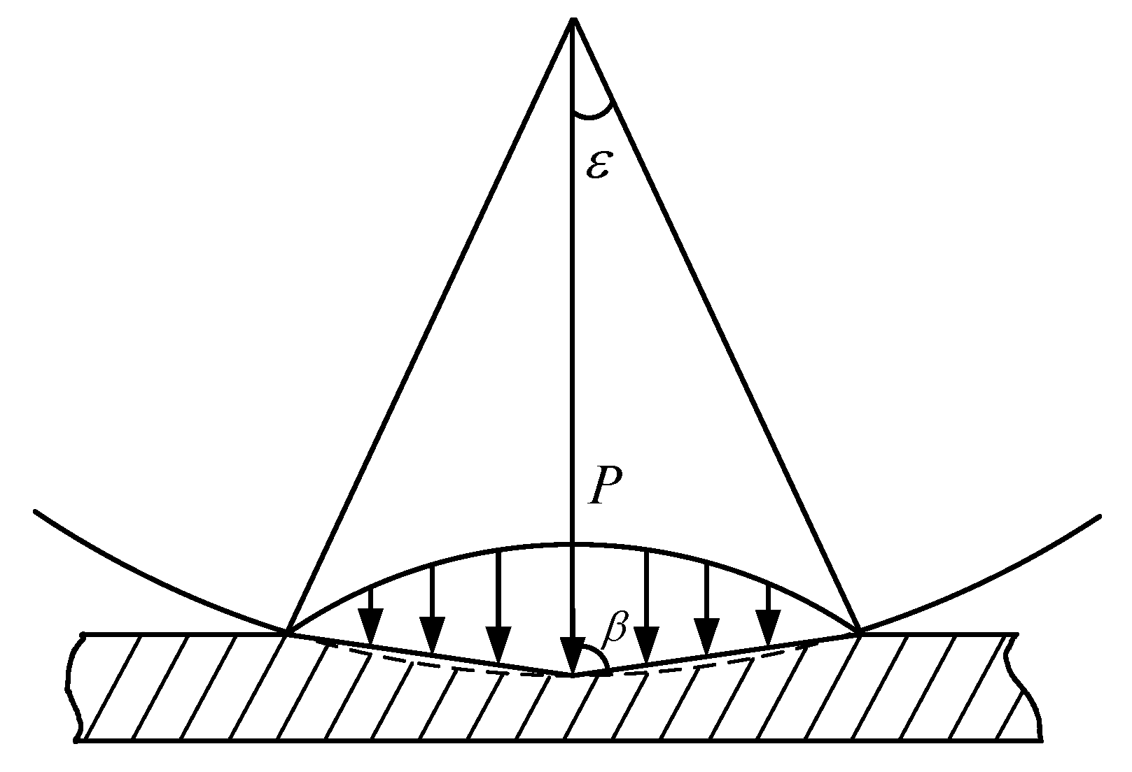
According to the improved Winkle model, the approximate contact model of considering joint clearance is show in Figure 1.

The contact boundary satisfies the relation as follow:

$$\cos \epsilon =\frac{\Delta R}{\Delta R+\delta }$$

(9)

where $\epsilon$ is half of contact angle, $\delta$ is the depth of the compression, $\Delta R=R_1-R_2$.

The relationship between chord length $l$ and compression depth chord $\epsilon$ as follow:

$$l=2R_2\sin \left(\frac{\epsilon }{2}\right)$$

(10)

Real contact area $A_r$ can be expressed as:

$$A_r=\lambda lb=2\lambda R_{2}b\sqrt{\frac{\delta }{2\left(\Delta R+\delta \right)}}$$

(11)

Substitute Equation (11) into Equation (8), The modified contact stiffness coefficient model is established as follows:

$$K_m=h_1{\Psi }^{(D-1)}{\left(A_r\right)}^{\left(D-1\right)/2}\left[{\Psi }^{\left(2-D\right)}-{a_c^{\prime }}^{\left(2-D\right)/2}\right]+h_2{\Psi }^{(D-1)}+h_3{h}_4{\Psi }^{(D-1)}$$

(12)

where $\Psi ={\left(\lambda mb{R}_2\frac{\delta }{2\left(\Delta R+\delta \right)}\right)}^{1/2}$, $\lambda$ is the area proportional coefficient, $b$ is the contact width, $\delta$ is the deformation of the rotating shaft and the sleeve, and $\Delta R=R_1-R_2$.

From Equation (12), it can be seen that the contact stiffness $K_m$ varies with the actual contact area $A_r$ .The actual contact area $A_r$ should be less than the nominal contact area $A$. $\lambda$ is defined as the area scale factor, which is less than 1. The relationship between $A_r$ and $A$ can be expressed as $A_r=\lambda A$.

$\lambda$ can be described as:

$$\lambda ={\left[\frac{{(\frac{3}{4E^{*}}\frac{R_1{R}_2}{R_1-R_2})}^{\frac{2}{3}}}{4(R_1^2-R_2^2)}\right]}^{\frac{2}{R_2}-\frac{2}{R_1}}$$

(13)

In recent years, many scholars have established contact models of asperities based on micro-contact theory, but few have considered the elastic–plastic deformation stage of asperities in the deformation process. The influence of normal contact damping on the contact force model is usually ignored. The new normal contact damping model is described as follows.

The deformation process of the asperities is divided into three stages: elastic deformation, elastic–plastic deformation, and plastic deformation. The elastic–plastic deformation can be divided into the first stage and the second stage. The deformation in the first stage of elastic–plastic deformation is elastic deformation, while the deformation in the second stage of elastic–plastic deformation is plastic deformation. The asperities convert energy into elastic potential energy during elastic deformation, and the energy is lost when plastic deformation occurs. The elastic potential energy and energy loss of the asperities can be calculated by integration.

The elastic deformation stage: according to Hertz theory, the normal $P_e$ loads of asperities can be expressed as:

$$P_e=\frac{4}{3}E{R}^{1/2}{\omega }^{3/2}, \omega <{\omega }_c$$

(14)

The potential energy at the elastic deformation stage of the asperities is expressed as:

$$w_{e1}={\displaystyle {\int }_0^{\omega }{P}_e}d\omega$$

(15)

The elastic–plastic deformation stage: when the deformation of the asperities is within the range of ${\omega }_c\le \omega \le 110{\omega }_c$, the asperities undergo elastic–plastic deformation. The deformation at this stage can be divided into the first stage of elastic-plastic deformation (${\omega }_c\le \omega \le 6{\omega }_c$) and the second stage of elastic–plastic deformation ($6\omega c\le \omega \le 110{\omega }_c$).

In the first stage of elastic–plastic deformation, the normal load of the asperities is expressed as:

$$P_{ep1}=\frac{2.06}{3}KH\pi R\frac{{\omega }^{1.425}}{{\omega }_c{}^{0.425}}$$

(16)

The potential energy in the first stage of the elastoplastic asperities is expressed as:

$$w_{e2}={\displaystyle {\int }_0^{\omega }{P}_{ep1}}d\omega$$

(17)

In the second stage of elastic–plastic deformation, the normal load of the asperities is expressed as:

$$P_{ep2}=\frac{2.8}{3}KH\pi R\frac{{\omega }^{1.263}}{{\omega }_c{}^{0.263}}$$

(18)

The energy loss in the second stage of the asperities is expressed as:

$$w_{p1}={\displaystyle {\int }_0^{\omega }{P}_{ep2}}d\omega$$

(19)

The condition of plastic deformation stage is $\omega >110{\omega }_c$, which means that the asperities have undergone plastic deformation. The normal load is expressed as:

$$P_p=2\pi \omega RH,w_{p2}={\displaystyle {\int }_0^{\omega }{P}_p}d\omega$$

(20)

From the distribution function of the asperities, the total elastic potential energy of the contact surface can be calculated as:

$$W_e={\displaystyle {\int }_{a_c}^{a_l}{w}_{e1}(a)n(a)da+}{\displaystyle {\int }_{{(\frac{1}{6})}^{\frac{1}{D-2}}{a}_c}^{a_l}{w}_{e2}(a)n(a)da}$$

(21)

where $a_L$ is the contact area of the largest asperity.

$a_L$ is expressed as:

$$a_L=\frac{2-D}{D}{A}_r$$

The total energy loss of the contact surface is expressed as:

$$W_p={\displaystyle {\int }_{{(\frac{1}{100})}^{\frac{1}{D-2}}{a}_c}^{{(\frac{1}{6})}^{\frac{1}{D-2}}{a}_c}{w}_{p1}(a)n(a)da+}{\displaystyle {\int }_0^{{(\frac{1}{100})}^{\frac{1}{D-2}}{a}_c}{w}_{p2}(a)n(a)da}$$

(22)

The damping factor is expressed as:

$$\eta =\frac{Wp}{We}$$

(23)

According to the literature [44], the normal damping coefficient can be expressed as:

$$C_n=\eta \sqrt{M{K}_m}$$

(24)

where M is the mass of base body with rough surface.

The new contact–collision force model is expressed as:

$$F_n=K_m{\delta }^n+D_m\dot{\delta }$$

(25)

where $F_n$ is the normal contact force, $K_m$ is the equivalent contact stiffness, $\delta$ is the normal penetration depth of contact position, $\dot{\delta }$ is the normal relative velocity at the contact point, n is the force index, and $D_m$ is the modified damping coefficient.

$D_m$ can be described as:

$$D_m=D_n+C_n$$

(26)

where $D_n$ is the damping coefficient, $D_n=\frac{3K(1-c_e^2){\delta }^n}{4{\dot{\delta }}^{(-)}}$, $c_e$ is the coefficient of restitution, and ${\dot{\delta }}^{(-)}$ is the relative velocity of the normal direction before the rotating shaft collides with the sleeve.

This part describes the process of establishing the modified contact model, where the contact stiffness coefficient and the damping coefficient are modified.

2.2. The Friction Model

The modified Coulomb friction model is suitable for the analysis of dynamics with clearance and impact [45]. Therefore, it is adopted as the friction model between the rotating shaft and the sleeve, which is expressed as:

$${\mathit{F}}_t=-{\mu }_t{c}_d{\mathit{F}}_n\frac{{\mathbf{\nu }}_t}{v_t}$$

(27)

where ${\mu }_t$ is the sliding friction coefficient, $v_t$ is the tangential velocity, and $c_d$ is the dynamic correction factor.

$c_d$ can be expressed as:

$$c_d=\{\begin{array}{ll}0& {\nu }_t\le v_0\\ \frac{{\nu }_t-{\nu }_0}{{\nu }_m-{\nu }_0}& v_0\le {\nu }_t\le v_m\\ 1& {\nu }_t\ge v_m\end{array}$$

(28)

where $v_0$ is the tangential velocity before the collision and $v_m$ is the velocity after the collision.

2.3. Collision Force Model of Revolute Joint with Clearance

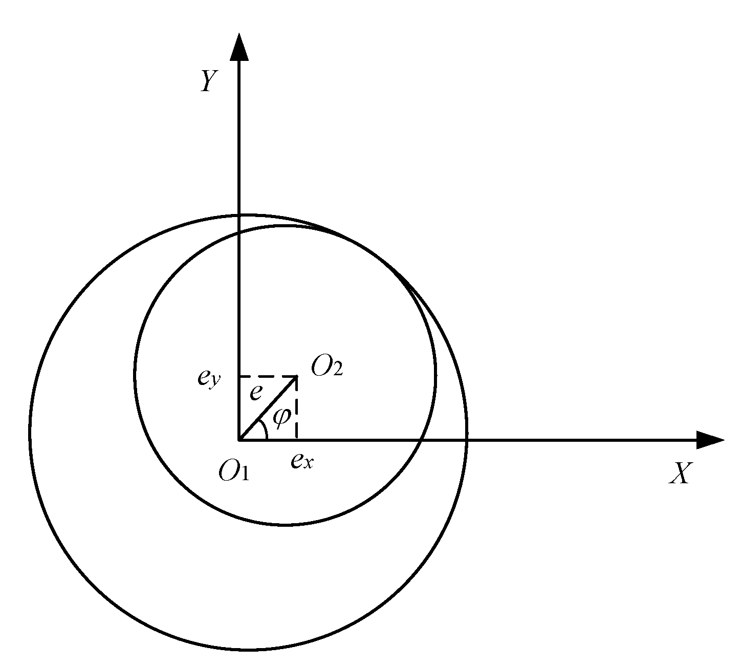
To facilitate the study, the clearance of the revolute joint was simplified to the clearance between the rotating shaft and the sleeve, as shown in Figure 2. The center distance $O_1{O}_2$ between the rotating shaft and the shaft sleeve is denoted as vector $e_i$. The projection of the clearance vector in the X axis direction is denoted as $e_{ix}$, and the projection of the clearance vector in the Y axis direction is denoted as $e_{iy}$.

When the rotating shaft is in contact with sleeve, the normal deformation at the contact point is denoted as ${\delta }_i$. ${\delta }_i$ can be described as:

$${\delta }_i=e_i-c_i$$

(29)

where $c_i=R_{i1}-R_{i2}$, $R_{i1}$ represents the radius of the sleeve, $R_{i2}$ represents the radius of the rotating shaft, and $c_i$ represents the ideal clearance.

A step function is introduced to determine whether a contact collision has occurred, which is as follows:

$$u\left({\delta }_i\right)=\{\begin{array}{ll}1& {\delta }_i\ge 0\\ 0& {\delta }_i<0\end{array}$$

(30)

According to the modified L–N contact force model, the collision force model can be described as:

$$F_n^{\prime }=\mu (\delta )F_n$$

(31)

When contact collision occurs between the rotating shaft and the sleeve, the normal velocity and tangential velocity are described as:

$$\{\begin{array}{c}{v}_{in}={\dot{e}}_{ix}\cos \phi -{\dot{e}}_{iy}\sin \phi \\ v_{it}={\dot{e}}_{iy}\cos \phi -{\dot{e}}_{ix}\sin \phi +\dot{\theta }{R}_2\end{array}$$

(32)

The projection of the contact force vector in the X axis direction and the projection of the contact force vector in the Y axis direction are expressed as:

$$\{\begin{array}{c}{F}_{ix}=u\left({\delta }_i\right)\left(F_{in}\cos \phi +F_{it}\sin \phi \right)\\ F_{iy}=u\left({\delta }_i\right)\left(F_{in}\sin \phi -F_{it}\cos \phi \right)\end{array}$$

(33)

where $F_{in}$ and $F_{it}$ represent the normal collision force and the tangential friction force of the ith joint, respectively.

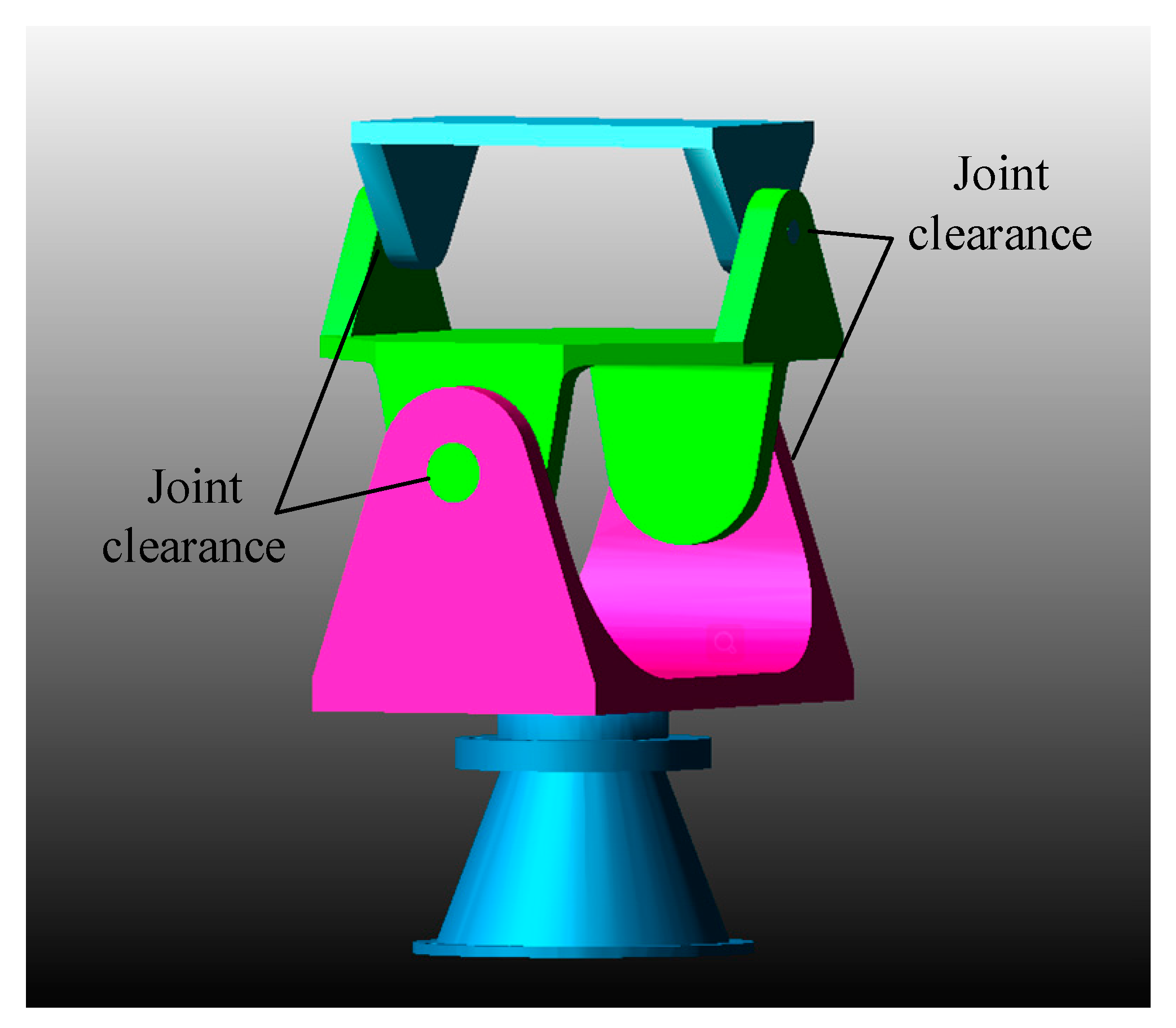
2.4. Dynamic Modeling of X–Y Pointing Mechanism with Clearance

The X–Y pointing mechanism has two rotational degrees of freedom, and the 3D model is shown in Figure 3. Based on the Newton–Euler approach, the process of establishing the dynamic model of the pointing mechanism is as follows.

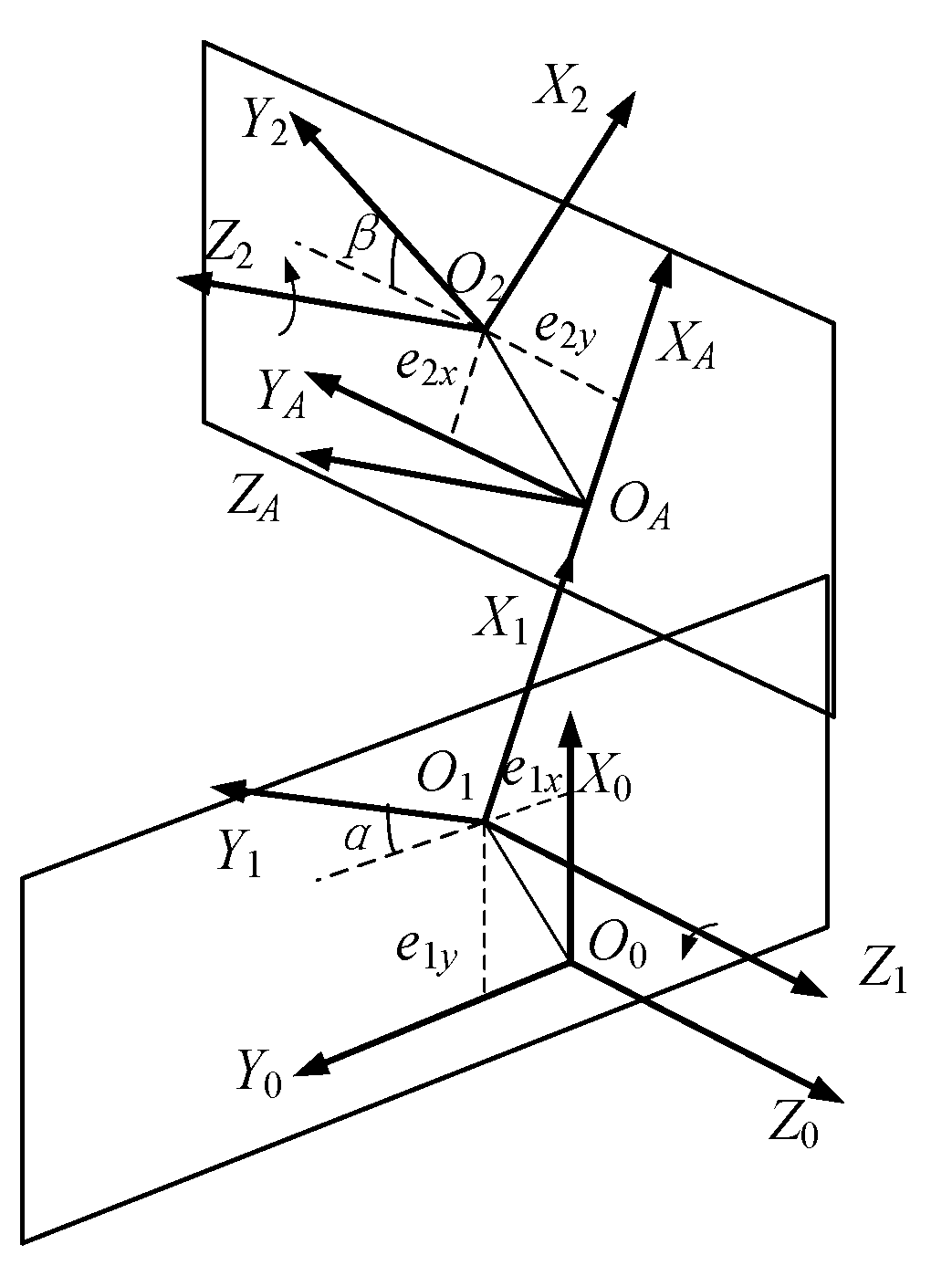
The coordinate systems of simplified pointing mechanism are shown in Figure 4. The reference coordinate system is $O_0-X_0{Y}_0{Z}_0$. $O_0$ is the origin of the reference coordinate system, the $Z_0$ axis is coincident with the axis of shafting 1, the $X_0$ axis is parallel and opposite to the direction of gravity, and the $Y_0$ axis is determined by the right-hand rule. The coordinate system of link 1 is $O_1-X_1{Y}_1{Z}_1$. $O_1$ is the origin of the coordinate system. The projection of $O_0{O}_1$ in the X₀axis direction is $e_{1x}$, and the projection of $O_0{O}_1$ in the Y₀ axis direction is $e_{1y}$. In the same way, the coordinate system of shafting 2 can be established such that $\alpha$ represents the rotational angle of shafting 1 and $\beta$ represents the rotational angle of shafting 2.

According to the literature [32], the dynamic equations are written in a standard form:

$$\mathbf{\tau }=\mathit{M}(q)\ddot{\mathit{q}}+\mathit{C}(q,\dot{q})+\mathit{G}(q)+{\mathbf{\tau }}_f$$

(34)

where $\mathit{q}$, $\dot{\mathit{q}}$, and $\ddot{\mathit{q}}$ are the 2-vectors; $\mathit{q}=[\alpha \beta {]}^T$; $\dot{\mathit{q}}=[\dot{\alpha }\dot{\beta }{]}^T$; $\ddot{\mathit{q}}={[\ddot{\alpha }\ddot{\beta }]}^T$; $\mathbf{\tau }$ is the 2-vector of actuator torques; $\mathit{M}(q)$ is the inertia matrix, which is symmetric and positively definite; $\mathit{C}(q,\dot{q})$ is the matrix of Coriolis force and centrifugal force; $\mathit{G}(q)$ is the gravity matrix depending on the pose of the pointing mechanism; and ${\mathbf{\tau }}_f$ is the friction torque.

$$\begin{array}{l}\mathit{M}(q)=\left[\begin{array}{cc}{I}_{1zz}-I_{2zx}\sin \beta -I_{2yz}\cos \beta & I_{2zz}\\ I_{2zx}\sin \beta -I_{2zy}\cos \beta & I_{2zz}\end{array}\right]\\ \mathit{C}(q,\dot{q})=\left[\begin{array}{c}\begin{array}{l}-I_{2zx}\dot{\alpha }\dot{\beta }\cos \beta +I_{2yz}\dot{\alpha }\dot{\beta }\sin \beta +\dot{\alpha }\cos \beta (I_{2xy}\dot{\alpha }\cos \beta -I_{2xz}\dot{\beta }+I_{2xx}\dot{\alpha }\sin \beta )\\ +m_2(L_1+e_{2x})(2\dot{\beta }{e}_{2x}+L{s}_2{\dot{\beta }}^2-\sin \beta ((-L_1-e_{2y}){\dot{\alpha }}^2-2{\dot{e}}_{1y}\dot{\alpha })+L{s}_2{\dot{\alpha }}^2\sin \\ \beta \cos \beta )+\dot{\alpha }\sin \beta (I_{2yy}\dot{\alpha }\cos \beta -I_{2yz}\dot{\beta }+I_{2xy}\dot{\alpha }\sin \beta )+L{s}_2{m}_2(2\dot{\beta }{\dot{e}}_{2x}+L{s}_2\\ {\dot{\beta }}^2-\sin \beta ((-L_1-e_{2y}){\dot{\alpha }}^2-2{\dot{e}}_{1y}\dot{\alpha }+{\ddot{e}}_{1x})+L{s}_2{\dot{\alpha }}^2\cos \beta \sin \beta )+L{s}_1{m}_1(-L{s}_1\\ {\dot{\alpha }}^2-2{\dot{e}}_{1y}\dot{\alpha })\end{array}\\ \begin{array}{l}-I_{2zx}\dot{\alpha }\dot{\beta }\cos \beta +I_{2zy}\dot{\alpha }\dot{\beta }\sin \beta -\dot{\alpha }\cos \beta (I_{2xy}\dot{\alpha }\cos \beta -I_{2xz}\dot{\beta }+I_{2xx}\dot{\alpha }\sin \beta )+\\ \dot{\alpha }\sin \beta (I_{2yy}\dot{\alpha }\cos \beta -I_{2yz}\dot{\beta }+I_{2yx}\dot{\alpha }\sin \beta )+L{s}_2{m}_2(2\dot{\beta }{\dot{e}}_{2x}+L{s}_2{\dot{\beta }}^2-\sin \beta \\ ((-L_1-e_{2y}){\dot{\alpha }}^2-2{\dot{e}}_{1y}\dot{\alpha })+L{s}_2{\dot{\alpha }}^2\cos \beta \sin \beta )\end{array}\end{array}\right]\\ \mathit{G}(q)=\left[\begin{array}{c}{m}_2(L_1+e_{2x})({\ddot{e}}_{2y}-\sin \beta ({\ddot{e}}_{1x}+g\cos \alpha ))+L{s}_2{m}_2({\ddot{e}}_{2y}-\sin \beta (+{\ddot{e}}_{1x}+g\cos \alpha ))+L{s}_1{m}_1({\ddot{e}}_{1x}+g\cos \alpha )\\ L{s}_2{m}_2({\ddot{e}}_{2y}-\sin \beta ({\ddot{e}}_{1x}+g\cos \alpha ))\end{array}\right]\\ {\mathbf{\tau }}_f=\left[\begin{array}{c}{F}_{t_1}{d}_1/2\\ F_{t_2}{d}_1/2\end{array}\right]\end{array}$$

Extracting the parameters to be identified, Equation (34) can be expressed as:

$$\mathbf{\tau }=\left[\begin{array}{l}{\tau }_1\\ {\tau }_2\end{array}\right]=\mathbf{\xi }\cdot \mathit{p}$$

(35)

where $\mathbf{\xi }=\left[\begin{array}{c}{\mathbf{\xi }}_{11}{\mathbf{\xi }}_{12}\\ {\mathbf{\xi }}_{21}{\mathbf{\xi }}_{22}\end{array}\right]$ is the observation matrix, ${\mathit{p}=\left[{\mathit{p}}_1{\mathit{p}}_2\right]}^T$ represents the parameters to be identified, and ${\mathit{p}}_i=\left[\begin{array}{ccccccccc}{I}_{xxi}& I_{xyi}& I_{xyi}& I_{yyi}& I_{yzi}& I_{zzi}& m_{i}L{s}_i& m_{\mathrm{i}}& F_{t_i}\end{array}\right]$

$${\mathbf{\xi }}_{11}=\left[\begin{array}{ccccccccc}0& 0& 0& 0& 0& \ddot{\alpha }& L{\mathbf{s}}_1(-L{\mathbf{s}}_1{\dot{\alpha }}^2-2{\dot{e}}_{1y}\dot{\alpha }+{\ddot{e}}_{1x}+g\cos \alpha )& 0& 0\end{array}\right]$$

$${\mathbf{\xi }}_{21}=\left[\begin{array}{ccccccccc}0& 0& 0& 0& 0& 0& 0& 0& 0\end{array}\right]$$

$${\xi }_{12}=\left[\begin{array}{l}\dot{\alpha }\sin \beta \dot{\alpha }\cos \beta \dot{\alpha }\cos \beta \dot{\alpha }\cos \beta +\dot{\alpha }\sin \beta \dot{\alpha }\sin \beta -\ddot{\alpha }\sin \beta -2\dot{\alpha }\dot{\beta }\cos \beta \dot{\alpha }\sin \beta \dot{\alpha }\cos \beta \\ -\ddot{\alpha }\cos \beta \ddot{\beta }(L_1+e_{2x})(\ddot{\alpha }\cos \beta -2\dot{\alpha }\dot{\beta }\sin \beta )+{\ddot{e}}_{1y}+2\dot{\alpha }{\dot{e}}_{1x}-g\sin \alpha +(L_1+e_{2x})\ddot{\alpha }+\\ L{s}_2\ddot{\alpha }\cos \beta +2\dot{\alpha }d{e}_{2x}\cos \beta -2\dot{\alpha }d{e}_{2y}\sin \beta -2L{s}_2\dot{\alpha }\dot{\beta }\sin \beta (L_1+e_{2x})({\ddot{e}}_{1y}+2\dot{\alpha }{\dot{e}}_{1x}-g\sin \alpha +\\ \ddot{\alpha }(L_1+e_{2x})+2\dot{\alpha }{\dot{e}}_{2x}\cos \beta -2\dot{\alpha }{\dot{e}}_{2y}\sin \beta )d_1/2\end{array}\right]$$

$${\mathbf{\xi }}_{22}=\left[\begin{array}{c}-{\dot{\alpha }}^2\cos \beta \sin \beta {\dot{\alpha }}^2({\sin }^2\beta -{\cos }^2\beta )-\ddot{\alpha }\sin \beta {\dot{\alpha }}^2\sin \beta \cos \beta -\ddot{\alpha }\cos \beta \ddot{\beta }{\ddot{e}}_{2y}+\\ 2\dot{\beta }{\dot{e}}_{2x}+L{s}_2{\dot{\beta }}^2-\sin \beta ((-L_1-e_{2y}){\dot{\alpha }}^2-2{\dot{e}}_{1y}\dot{\alpha }+{\ddot{e}}_{1x}+g\cos \alpha )+L{s}_2{\dot{\alpha }}^2\cos \beta \sin \beta 0d_2/2\end{array}\right]$$

where $L{s}_1$ is the distance between the center of mass of link 1 and $O_1$, $L{s}_2$ is the distance between the center of mass of link 2 and $O_2$, $L_1$ is the length of link 1, $L_2$ is the length of link 2, $e_{1x}$ and $e_{1y}$ is the clearance of joint 1, $e_{2x}$ and $e_{2y}$ is the clearance of joint 2. m_i is the mass of link i. $I_{xxi},I_{xyi},I_{xzi},I_{yyi},I_{yzi},I_{zzi}$ are parameters of the inertial matrix of link i.

When the input trajectories are given, the input torques can be obtained based on the simulation. $\xi$ can be obtained through the dynamic model [32]. Then the dynamic parameter identification can be carried out based on identification algorithm.

3. Excitation Trajectory of the X–Y Pointing Mechanism

The finite Fourier series was used as the periodic excitation. The joint trajectory of the X–Y pointing mechanism can be expressed as:

$$q_i(t)={\displaystyle \sum _{k=1}^N(a_{i,k}sin(k{\omega }_{f}t)+b_{i,k}\cos (k{\omega }_{f}t))}+q_{i,0}$$

(36)

In order to ensure the X–Y pointing mechanism motions in a reasonable space, the velocity and acceleration were set to zero at the starting and the ending points and the velocity was set to never exceed the maximum velocity. The boundary conditions of each joint are set as follows:

$$\{\begin{array}{l}\left|q_1(t)\right|\le 1.2\mathrm{rad};\left|q_2(t)\right|\le 1\mathrm{rad};\\ \left|{\dot{q}}_1(t)\right|\le 0.25\mathrm{rad}/s;\left|{\dot{q}}_2(t)\right|\le 0.2\mathrm{rad}/s\\ \left|{\ddot{q}}_1(t)\right|\le 1\mathrm{rad}/s^2;\left|{\ddot{q}}_2(t)\right|\le 1\mathrm{rad}/s^2\\ q_i\left(t_0\right)=q_i\left(t_f\right)=0\\ {\dot{q}}_i\left(t_0\right)={\dot{q}}_i\left(t_f\right)=0\\ {\ddot{q}}_i\left(t_0\right)={\ddot{q}}_i\left(t_f\right)=0\end{array},\forall i,t$$

(37)

The optimal excitation trajectory can accurately estimate the relevant inertia parameters of the mechanism under the disturbance of external signals. The authors of this paper adopted the method of the matrix condition number to carry out the trajectory optimization. Based on the finite Fourier series model, the minimum condition number was chosen as the optimization goal. In the process of motion, the position, velocity, and acceleration should satisfy the constraints and the motion should fill the entire working space of the mechanism as much as possible. The calculation formula of the conditional number of matrix is expressed as:

$$cond(\mathit{A})=\Vert \mathit{A}\Vert \Vert {\mathit{A}}^{-1}\Vert$$

(38)

In order to solve the ill-conditioned problem of the matrix, the matrix singular value is used to express the condition number. The condition number can be expressed as:

$$cond(\xi )=\frac{{\sigma }_{\max }(\xi )}{{\sigma }_{\min }(\xi )}$$

(39)

where ${\sigma }_{\max }(\xi )$ is the maximum singular value and ${\sigma }_{\min }(\xi )$ is the minimum singular value.

The minimization of Equation (39) can be solved by the fmincon function in MATLAB.

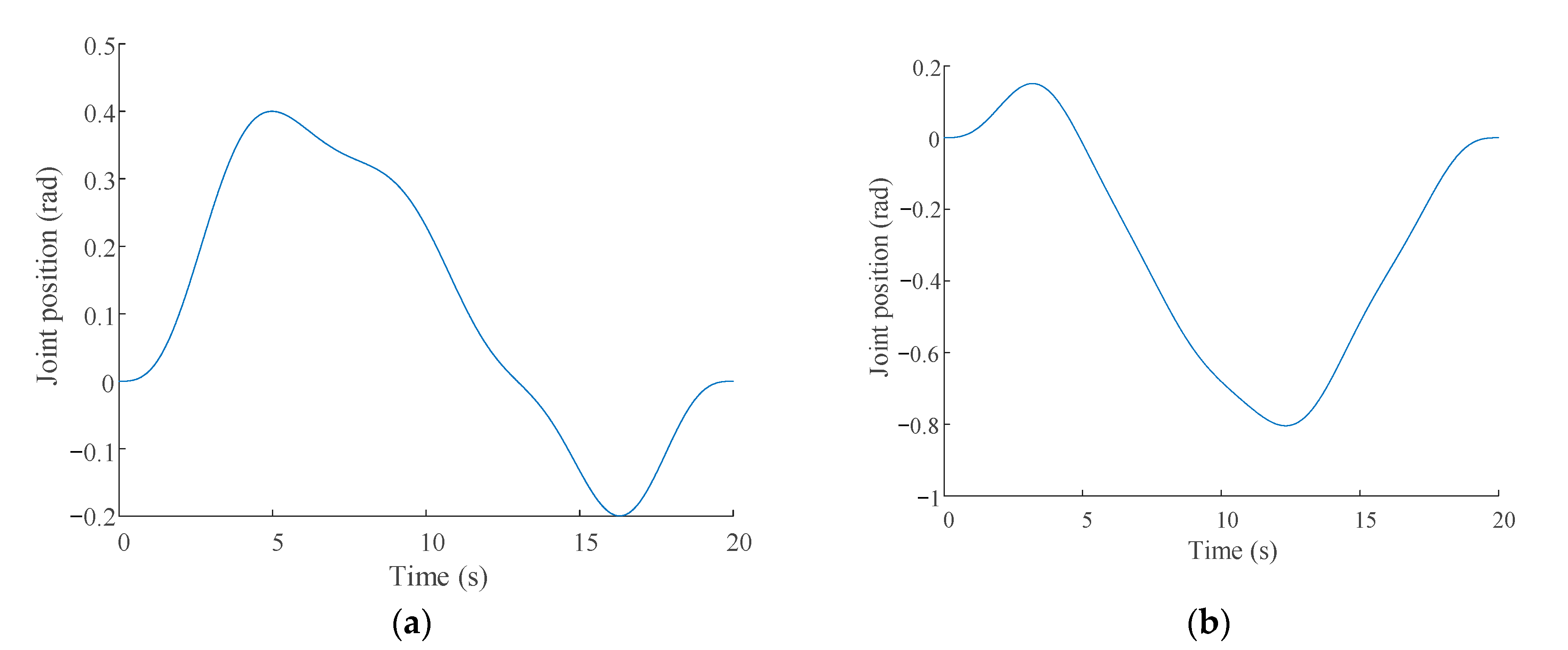
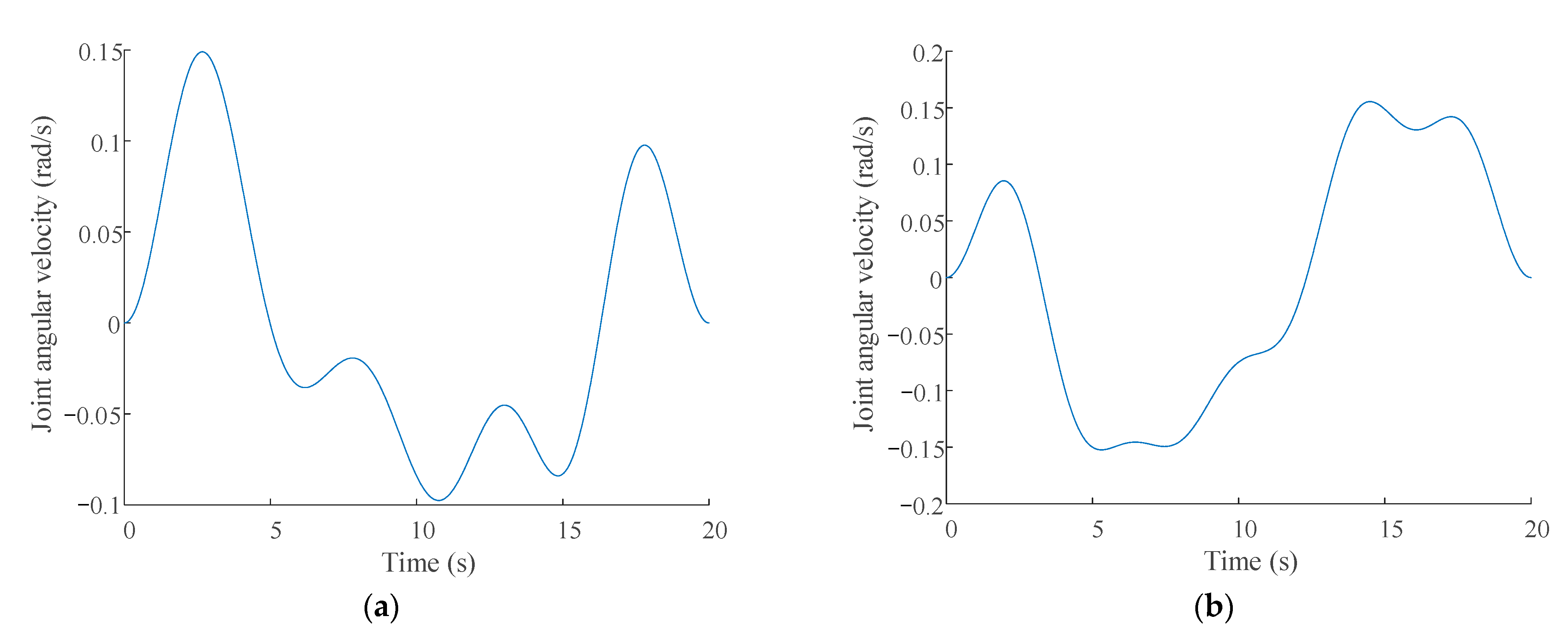
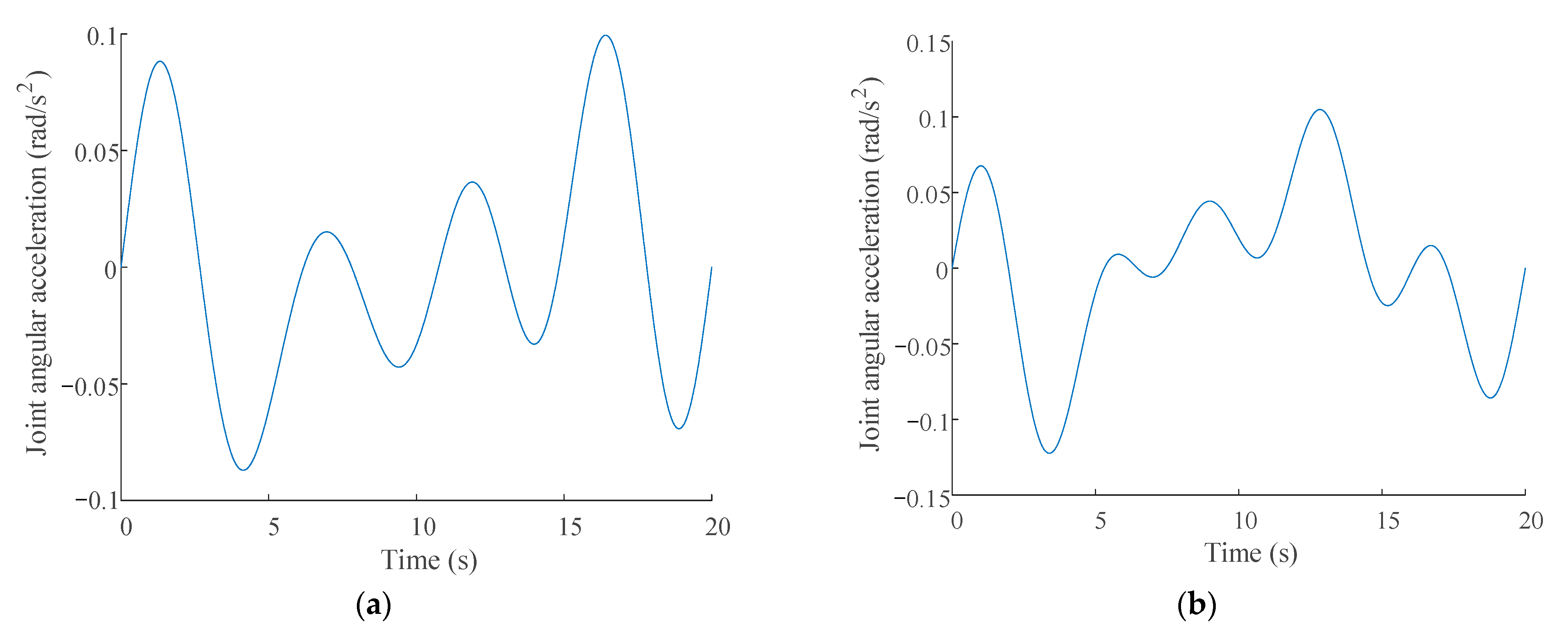
The optimized excitation trajectory parameters are shown in

Table 1. Excitation trajectory parameters.

Link Number i	Parameter Number k	${\mathit{q}}_{\mathit{i},\mathit{k}}$	${\mathit{a}}_{\mathit{i},\mathit{k}}$	$b_{i,k}$
1	1	0.111	0.243	−0.113
	2		−6.5 × 10−10	−0.01
	3		−0.028	0.001
	4		−0.033	0.013
	5		−0.005	−0.003
2	1	−0.306	0.251	0.372
	2		−0.029	−0.037
	3		−0.016	−0.033
	4		−0.015	0.003
	5		−0.017	0.001

. After putting the parameters into the Fourier series, the motion trajectory, velocity, and acceleration were be obtained, as shown in Figure 5, Figure 6 and Figure 7.

It can be seen from Figure 5, Figure 6 and Figure 7 that the excitation trajectories of the X–Y pointing mechanism were relatively smooth. The trajectories passed through most of the working space, and the motion of each joint was within the constraint range. It was further proved that when the excitation trajectories were adopted as finite Fourier series, the joint angular velocities, joint angular accelerations, and joint torques of the X–Y pointing mechanism maintained stable working conditions. The trajectories had good anti-interference performance.

4. Dynamic Parameter Identification of the Pointing Mechanism

4.1. ABC Algorithm

The ABC algorithm is an intelligent algorithm that simulates the behavior of a bee colony searching for nectar. It can avoid falling into local optimization, and it is an effective tool to find global optimum parameters.

The specific solution process of the algorithm is as follows:

(1) The ABC algorithm parameters are set. The population number NP, the maximum iteration number G, and the range of solution are set first. Within the search range, the initial position $x_i$ (i = 1, 2, 3, …, SN) is randomly generated, where SN is the number of food sources. Each solution is a D-dimensional vector, where D is the dimensionality of the solution. When executing tth operation, the position of the food source i is $x_i^t=\left[x_{i1}^t,x_{i2}^t,x_{i3}^t\cdots x_{iD}^t\right]$, where t represents the current iteration number. According to Equation (40), the population can be initialize as:

$$x_{id}=x_d^{\min }+\mathrm{rand}\left(x_d^{\max }-x_d^{\mathrm{mix}}\right)$$

(40)

(2) The search phase is conducted. Each employed bee updates the new location information of the food sources according to Equation (41) and calculates the fitness $fit$ of the new nectar source location according to Equation (42). If the fitness value is better than the old fitness value, the new location information of the food sources should be used to replace the old one according to the greedy selection method; otherwise, the location information of the old one should be retained.

$$v_{id}=x_{id}+\mathrm{rand}\left(x_{id}-x_{jd}\right)$$

(41)

$$fit=\min \left|{\tau }^{\prime }-\tau \right|$$

(42)

(3) After the employed bees complete the search process, they share the food source location information with onlookers. Then, according to the location information of the food sources shared by the employed bees, the onlookers calculate the probability and judge whether to follow the employed bees according to Equation (43). If it falls into a local optimum, the location information of food sources is abandoned.

$$p_i=\frac{fi{t}_i}{{\displaystyle {\sum }_{i=1}^{SN}fi{t}_i}}$$

(43)

(4) In the search process, if the food source X_i reaches the search threshold after n iterative searches but there is no better food source found, the food sources are discarded and the role of employed bees changes to that of reconnaissance bees. The reconnaissance bees randomly generate new food source location information to replace X_i in the search range. The process is expressed as:

$$x_i^{t+1}=\{\begin{array}{l}{x}_d^{\min }+\mathrm{rand}\left(x_d^{\max }-x_d^{\mathrm{mix}}\right),tria{l}_i\ge \mathrm{limit}\\ x_i^t,tria{l}_i<\mathrm{limit}\end{array}$$

(44)

(5) The best food sources are stored.

(6) Whether the abort condition is met is judged. If the condition is met, the optimal solution is output; otherwise, the program goes to step (2).

According to the excitation trajectories and Equation (35), dynamic parameter identification can be carried out by the ABC algorithm.

4.2. Dynamic Simulation and Parameter Identification

The pointing mechanism model that considers revolute joint clearance was established in the Adams software, and the optimized excitation trajectory in Section 3 was introduced into the model as the input. After the dynamic simulation, the driving toques could be obtained.

The ABC algorithm was used to identify the dynamic parameters of the X–Y pointing mechanism. Firstly, the relevant parameters in the program were initialized. Reasonable parameters could make the program run stably. The nectar search range was set to ±10%. of the initial value. Some important parameters are shown in

Table 2. Parameter settings of the artificial bee colony (ABC) algorithm.

Parameter	Initial Value	Remarks
MaxIt	200	Number of population iterations
Npop	100	Number of employed bees
Nonlooker	100	Number of onlookers
a	0.5	Acceleration factor
Nvar	10/3	Number of food sources: shafting 1, 3; shafting 2, 10.
L	600	Experimental constraints of food sources

. Secondly, program files for dynamic parameter identification were written. Finally, the optimal solution was obtained by searching for the best food sources.

4.3. Results and Discussion

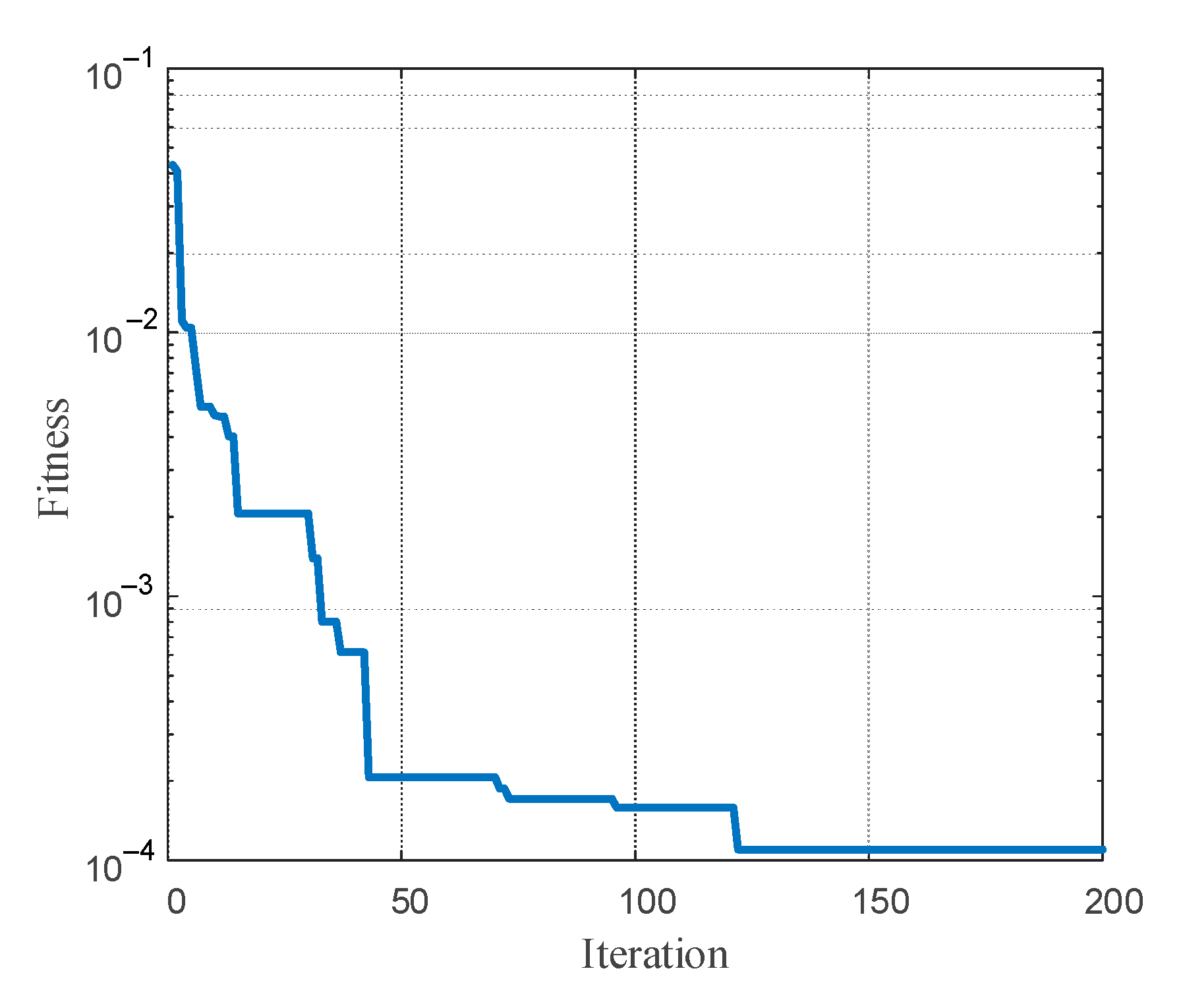
Parameter identification was carried out with the ABC algorithm in MATLAB 2018b programming environment on an Advanced Micro Devices (AMD) Core R5-4600U PC running Windows 10. No toolbox was used. In a certain range, as the size of bees increased, the algorithm generated better results. The maximum number of iterations was set to 200. When the fitness value was less than 10⁻⁶, the operation was completed. The number of employed bees was 100, the number of onlookers was 100, and the acceleration factor was 0.5. The dynamic parameter identification and convergence process of the ABC algorithm is shown in Figure 8. When the number of iterations reached about 200, the fitness function gradually converged and the fitness value became less than 0.002. It can be seen that the dynamic parameter identification based on the ABC algorithm had the characteristics of a fast convergence speed and a high calculation accuracy.

After 200 iterations, a total of 11 groups of parameter identification results were obtained. The dynamic model that considered the clearance and the dynamic model that did not consider the clearance were used for identification. The results are shown in

Table 3. Parameter identification results.

Identification	System Value	Identification of Clearance Model	Ideal Model Identification	Error Ratio
$I_{xx2}$ (kg·m2)	0.00467	0.00685	0.00077	0.55897
$I_{xy2}$ (kg·m2)	0	0.00803	0.00343	2.34111
$I_{xz2}$ (kg·m2)	0	0.00296	0.00783	0.37803
$I_{yy2}$ (kg·m2)	0.00533	0.00967	0.00474	7.427356
$I_{yz2}$ (kg·m2)	0	0.00189	0.00340	0.55588
$I_{zz2}$ (kg·m2)	0.00181	0.00131	0.00640	0.10893
$m_2$ (kg)	0.8596	0.84191	0.82352	0.49029
$L{s}_2$ (m)	0.03419	0.03394	0.03274	0.17241
$I_{zz1}$ (kg·m2)	0.0175	0.00834	0.00486	0.72468
$L{s}_1$ (m)	2.1391	2.13699	2.08471	0.03879
$m_1$ (kg)	0.04821	0.04815	0.05241	0.01425

.

The error rate indicated the degree of similarity between the identification results and the system value. When the error rate was greater than 1, it was indicated that the identification result based on the dynamic model that did not consider the clearance was more accurate. When the error rate was less than 1, it was indicated that the identification result based on the dynamic model that considered the clearance was more accurate. From Table 3, it can be seen that the identification results based on the dynamic model that considered the clearance were more accurate and conformed to the actual situation. When the asperities, the clearance, and the contact–collision force were taken in consideration in the dynamic model, the dynamic model was more accurate. Based on the more accurate dynamic model, the dynamic parameter identification was more accurate as well. In a word, nearly all the dynamic parameter identification results were closer to the true values when the clearance was taken into consideration.

This study provides an insight into the effect of joint clearance on dynamic parameter identification. The clearance can affect the accuracy of the dynamic model, and the accuracy of the dynamic model can affect the accuracy of the dynamic parameter identification. Dynamic parameter identification that considers joint clearance is meaningful for the high-performance control of pointing mechanisms and other robots. More accurate dynamic model in this paper can describe the effect of joint clearance on joint torque, which can reduce the effect of joint clearance on dynamic identification accuracy. Compared with the dynamic parameter identification based on the dynamic model without considering the joint clearance, the dynamic parameter identification base on the more accurate dynamic model can improve the dynamic parameter identification accuracy.

5. Conclusions

The authors of this paper conducted the dynamic parameter identification of an X–Y pointing mechanism. The clearance of the revolute joint was considered in a nonlinear dynamic model. The contact stiffness and damping coefficients of a normal contact force model were modified based on fractal theory and elastoplastic theory, which improved the accuracy of the nonlinear dynamic model. In order to increase the anti-interference of the excitation trajectory, the excitation trajectory was optimized according to the constraint conditions. The Adams dynamic simulation software was used to simulate the dynamics of the pointing mechanism while considering the revolute joint clearance, and driving torques were obtained. According to the driving torques, the ABC algorithm was used to identify the dynamic parameters based on the dynamic model that considered the clearance and the dynamic model that did not consider the clearance. Compared with the identification result based on the dynamic model that did not consider the clearance and collision, the identification result based on the dynamic model that considered the clearance and collision was more accurate. This research provides a theoretical basis for improving dynamic parameter identification accuracy and high-precision control.

References

- Yu, J.; Wu, K.; Zong, G.; Kong, X. A Comparative Study on Motion Characteristics of Three Two-Degree-of-Freedom Pointing Mechanisms. J. Mech. Robot. 2016, 8, 021027. [Google Scholar] [CrossRef]
- Muhammad, A.; Jingjun, Y.; Yan, X.; Abdus, S. Conceptual design, modeling and compliance characterization of a novel 2-DOF rotational pointing mechanism for fast steering mirror. Chin. J. Aeronaut. 2020. [Google Scholar] [CrossRef]
- Wu, J.; Wang, J.; You, Z. An overview of dynamic parameter identification of robots. Robot. Comput. Integr. Manuf. 2010, 26, 414–419. [Google Scholar] [CrossRef]
- Qin, Z.; Baron, R.L.; Birglen, R. A new approach to the dynamic parameter identification of robotic manipulators. Robotica 2010, 28, 539–547. [Google Scholar] [CrossRef] [Green Version]
- Tourassis, V.D.; Neuman, C.P. The inertial characteristics of dynamic robot models. Mech. Mach. Theory 1985, 20, 41–52. [Google Scholar] [CrossRef]
- Vivas, A.; Poignet, P.; Marquet, F.; Gautier, M. Experimental dynamic identification of a fully parallel robot. In Proceedings of the IEEE International Conference on Robotics and Automation, Taipei, Taiwan, 14–19 September 2003; pp. 3278–3283. [Google Scholar]
- Bona, B.; Indri, M.; Smaldone, N. Rapid Prototyping of a Model-Based Control with Friction Compensation for a Direct-Drive Robot. IEEE ASME Trans. Mechatron. 2006, 11, 576–584. [Google Scholar] [CrossRef]
- Swevers, J.; Verdonck, W.; Schutter, J. Dynamic Model Identification for Industrial Robots. IEEE ASME Trans. Mechatron. 2007, 27, 58–71. [Google Scholar]
- Calanca, A.; Capisani, L.M.; Ferrara, A.; Magnani, L. MIMO closed loop identification of an industrial robot. IEEE Trans. Control Syst. Technol. 2010, 19, 1214–1224. [Google Scholar] [CrossRef]
- Atkeson, C.G.; An, C.H.; Hollerbach, J.M. Estimation of inertial parameters of manipulator loads and links. Int. J. Robot. Res. 1986, 5, 101–119. [Google Scholar] [CrossRef]
- Huo, X.; Lian, B.; Wang, P.; Song, T.; Sun, T. Dynamic identification of a tracking parallel mechanism. Mech. Mach. Theory 2020, 155, 104091. [Google Scholar] [CrossRef]
- Pukelsheim, F. Optimal Design of Experiments; The Society for Industrial and Applied Mathe Matics: New York, NY, USA, 2006; pp. 408–454. [Google Scholar]
- Swevers, J.; Ganseman, C.; De Schutter, J.; Van Brussel, H. Generation of periodic trajectories for optimal robot excitation. ASME J. Manuf. Sci. Eng. 1997, 119, 611–615. [Google Scholar] [CrossRef]
- Gautier, M. Optimal motion planning for robot’s inertial parameters identification. In Proceedings of the 31st IEEE Conference on Decision and Control, Tucson, AZ, USA, 16–18 December 1992; Volume 1, pp. 70–73. [Google Scholar]
- Armstrong, B. On finding exciting trajectories for identification experiments involving systems with nonlinear dynamics. Int. J. Robot. Res. 1989, 8, 28–48. [Google Scholar] [CrossRef]
- Karaboga, D. An Idea Based on Honey Bee Swarm for Numerical Optimization; Technical Report-tr06; Erciyes University: Kayseri, Turkey, 2005. [Google Scholar]
- Park, K.J. Fourier-based optimal excitation trajectories for the dynamic identification of robots. Robotica 2006, 24, 625. [Google Scholar] [CrossRef]
- Gautier, M.; Janot, A.; Vandanjon, P.O. A new closed-loop output error method for parameter identification of robot dynamics. IEEE Trans. Control Syst. Technol. 2013, 21, 428–444. [Google Scholar] [CrossRef] [Green Version]
- Gautier, M.; Poignet, P. Extended Kalman filtering and weighted least squares dynamic identification of robot. Control Eng. Pract. 2001, 9, 1361–1372. [Google Scholar] [CrossRef]
- Kozlowski, K.R. Modelling and Identification in Robotics; Springer: London, UK, 2012; pp. 47–81. [Google Scholar]
- Ha, I.J.; Ko, M.S.; Kwon, S.K. An efficient estimation algorithm for the model parameters of robotic manipulators. IEEE Trans. Robot. Automat. 1989, 5, 386–394. [Google Scholar] [CrossRef]
- Xuan, J.; Liu, J.G.; Zhu, S.F. Identification method of hydrodynamic parameters of autonomous underwater vehicle based on genetic algorithm. J. Mech. Eng. 2010, 46, 96–100. [Google Scholar]
- Ding, L.; Wu, H.; Yao, Y.; Yang, Y.X. Dynamic model identification for 6-DOF industrial robots. J. Robot. 2015, 2015. [Google Scholar] [CrossRef] [Green Version]
- Ding, L.; Wu, H.; Yao, Y. Chaotic artificial bee colony algorithm for system identification of a small-scale unmanned helicopter. Int. J. Aerosp. Eng. 2015, 2015. [Google Scholar] [CrossRef]
- Karaboga, D.; Basturk, B. On the performance of artificial bee colony (ABC) algorithm. Appl. Soft Comput. 2008, 8, 687–697. [Google Scholar] [CrossRef]
- Swevers, J.; Ganseman, C.; Tukel, D.B.; DeSchutter, J.; VanBrussel, H. Optimal robot excitation and identification. IEEE Trans. Robot. Automat. 1997, 13, 730–740. [Google Scholar] [CrossRef] [Green Version]
- Chen, X.; Jiang, S.; Wang, S.; Deng, Y. Dynamics analysis of planar multi-DOF mechanism with multiple revolute clearances and chaos identification of revolute clearance joints. Multibody Syst. Dyn. 2019, 47, 317–345. [Google Scholar] [CrossRef]
- Schwab, A.L.; Meijaard, J.P.; Meijers, P. A comparison of revolute joint clearance models in the dynamic analysis of rigid and elastic mechanical systems. Mech. Mach. Theory 2002, 37, 895–913. [Google Scholar] [CrossRef]
- Wang, Z.; Tian, Q.; Hu, H.; Flores, P. Nonlinear dynamics and chaotic control of a flexible multibody system with uncertain joint clearance. Nonlinear Dyn. 2016, 86, 1571–1597. [Google Scholar] [CrossRef]
- Chen, X.; Jia, Y.; Deng, Y.; Wang, Q. Dynamics behavior analysis of parallel mechanism with joint clearance and flexible links. Shock Vib. 2018, 2018. [Google Scholar] [CrossRef] [Green Version]
- Xiang, W.; Yan, S.; Wu, J. Dynamic analysis of planar mechanical systems considering stick-slip and Stribeck effect in revolute clearance joints. Nonlinear Dyn. 2019, 95, 321–341. [Google Scholar] [CrossRef]
- Erkaya, S. Effects of Joint Clearance on the Motion Accuracy of Robotic Manipulators. J. Mech. Eng. 2018, 64, 82–94. [Google Scholar]
- Flores, P.; Koshy, C.S.; Lankarani, H.M.; Ambrósio, J.; Claro, J.C.P. Numerical and experimental investigation on multibody systems with revolute clearance joints. Nonlinear Dyn. 2011, 65, 383–398. [Google Scholar] [CrossRef] [Green Version]
- Zhang, Z.; Xu, L.; Flores, P.; Lankarani, H.M. A Kriging model for dynamics of mechanical systems with revolute joint clearances. ASME J. Comput. Nonlinear Dynam. 2014, 9, 031013. [Google Scholar] [CrossRef]
- Li, K.L.; Tsai, Y.K.; Chan, K.Y. Identifying joint clearance via robot manipulation. Proc. Inst. Mech. Eng. C J. Mech. Eng. Sci. 2018, 232, 2549–2574. [Google Scholar] [CrossRef]
- Ruderman, M.; Hoffmann, F.; Bertram, T. Modeling and identification of elastic robot joints with hysteresis and backlash. IEEE Trans. Ind. Electron. 2009, 56, 3840–3847. [Google Scholar] [CrossRef]
- Erkaya, S.; Uzmay, I. Determining link parameters using genetic algorithm in mechanisms with joint clearance. Mech. Mach. Theory 2009, 44, 222–234. [Google Scholar] [CrossRef]
- Han, X.; Li, F.; Gao, Z.; Li, S. Dynamic Characteristics of Space Mechanism Considering Friction and Stiffness. CJME 2020, 56, 170–180. [Google Scholar]
- Whitehouse, D.J.; Archard, J.F. The Properties of Random Surfaces of Significance in their Contact. Proc. Math. Phys. Eng. Sci. 1971, 316, 97–121. [Google Scholar]
- Wang, S.; Komvopoulos, K. A Fractal Theory of the Interfacial Temperature Distribution in the Slow Sliding Regime: Part I—Elastic Contact and Heat Transfer Analysis. J. Tribol. 1994, 116, 812–822. [Google Scholar] [CrossRef]
- Li, S.; Han, X.; Wang, J.; Sun, J.; Li, F. Contact Model of Revolute Joint with Clearance Based on Fractal Theory. CJME 2018, 31. [Google Scholar] [CrossRef] [Green Version]
- Kogut, L.; Etsion, I. Elastic-plastic contact analy sis ofa sphere and a rigid flat. ASME J. 2002, 69, 657–662. [Google Scholar]
- Hertz, H. Ueber die Berührung fester elastischer Körper. J. Für Die Reine Und Angew. Math. 2006, 1882, 156–171. [Google Scholar]
- Majumdar, A.; Bhushan, B. Fractal Model of Elastic Lastic Contact between Rough Surfaces. ASME J. Tribol. 1991, 113, 1–11. [Google Scholar] [CrossRef]
- Flores, P.; Lankarani, H.M. Dynamic response of multibody systems with multiple clearance joints. ASME J. Comput. Nonlinear Dyn. 2012, 7, 031003. [Google Scholar] [CrossRef]
Figure 1.
Approximate contact model of considering joint clearance.
Figure 2.
Schematic diagram of the gap.
Figure 3.
The X–Y pointing mechanism with clearance.
Figure 4.
Coordinate system of the X–Y pointing mechanism with clearance.
Figure 5.
Rotational angle curves: (a) rotational angle curve of shafting 1 and (b) rotational angle curve of shafting 2.
Figure 6.
Angular velocity curves: (a) the angular velocity curve of shafting 1 and (b) the angular velocity curve of shafting 2.
Figure 7.
Angular acceleration curves: (a) the angular acceleration curve of shafting 1 and (b) the angular acceleration curve of shafting 2.
Figure 8.
Convergence effect of the ABC algorithm for dynamic parameter identification.