Globally Optimal Redundancy Resolution with Dynamic Programming for Robot Planning: A ROS Implementation


1
Department of Computer Engineering, Electrical Engineering and Applied Mathematics (DIEM), University of Salerno, 84084 Fisciano, Italy
2
Robotic Exploration, ALTEC S.p.A., 10146 Torino, Italy
*
Author to whom correspondence should be addressed.
Robotics 2021, 10(1), 42; https://0-doi-org.brum.beds.ac.uk/10.3390/robotics10010042
Submission received: 2 February 2021
/
Revised: 27 February 2021
/
Accepted: 1 March 2021
/
Published: 4 March 2021
(This article belongs to the Special Issue Advances in Industrial Robotics and Intelligent Systems)
Abstract
:Dynamic programming techniques have proven much more flexible than calculus of variations and other techniques in performing redundancy resolution through global optimization of performance indices. When the state and input spaces are discrete, and the time horizon is finite, they can easily accommodate generic constraints and objective functions and find Pareto-optimal sets. Several implementations have been proposed in previous works, but either they do not ensure the achievement of the globally optimal solution, or they have not been demonstrated on robots of practical relevance. In this communication, recent advances in dynamic programming redundancy resolution, so far only demonstrated on simple planar robots, are extended to be used with generic kinematic structures. This is done by expanding the Robot Operating System (ROS) and proposing a novel architecture meeting the requirements of maintainability, re-usability, modularity and flexibility that are usually required to robotic software libraries. The proposed ROS extension integrates seamlessly with the other software components of the ROS ecosystem, so as to encourage the reuse of the available visualization and analysis tools. The new architecture is demonstrated on a 7-DOF robot with a six-dimensional task, and topological analyses are carried out on both its state space and resulting joint-space solution.
1. Introduction
When a robot is redundant with respect to its task, the inverse kinematics problem admits an infinite set of solutions almost everywhere in its workspace. It results in augmented dexterity that can be exploited to achieve several objectives, which are usually desirable for a multitude of real applications, such as obstacle avoidance and constrained motions, improvement of manipulability and local or global optimization of generic performance indices [1]. Choosing the joint-space configuration in agreement with the criteria above for each point of the given end-effector trajectory is usually referred to as redundancy resolution.
Redundancy resolution via global optimization of performance indices is of particular interest in real applications as it allows saving resources, such as energy and time, and consequently maximizing the use of the robotic asset. On the other hand, such a technique requires time to provide a solution, therefore it is only suited for off-line planning scenarios. In space applications of exploration and construction, the minimization of energy translates into increasing the number of operations that can be completed within the available energy budget. In manufacturing industries, redundancy can be exploited to perform tasks as fast as possible, so as to increase the plant throughput. Both applications are characterized by an off-line programming approach, where the controller references either are generated a long time before they are executed, as in space applications with windowed communications, or are computed once and executed several times, as in automated manufacturing.
If the environment in which the robotic asset operates is subject to contingencies, there still is a chance to optimize the resources by coupling the off-line planner with an on-board planner. The latter should allow for the execution of the trajectory computed off-line, so that resources are still globally optimized, until some unplanned event arises, in which case the plan has to be modified. Yet the modifications could be implemented in a neighborhood of the globally optimal solution.
In the literature, the problem of maximizing or minimizing an integral function, subject to geometric or differential constraints, is addressed by making use of calculus of variations, either through the Euler-Lagrange formulation [2] or the Pontryagin’s maximum principle [3], dynamic programming (DP) [4,5], or other numerical optimization techniques, as by Shen et al. [6], among the others. Calculus of variations only provides necessary conditions for optimality and is, therefore, prone to sub-optimal solutions. Such conditions are given in the form of second-order differential equations and related boundary conditions. When initial and final joint positions are not assigned, velocities are constrained at the beginning and at the end of the trajectory. This results in a Two-Point Boundary Value Problem (TPBVP) made of a system of non-linear differential equations. Such problems rarely have a closed-form solution and numerical methods are usually employed [7,8]. Unfortunately, on the practical side, off-the-shelf numeric solvers do not guarantee the achievement of a solution, if it exists, and the successful computation might depend on a suitable choice of an initial guess [7]. Lastly, the equations that make up the TPBVP can be derived from Euler-Lagrange or Pontryagin’s Maximum Principle necessary conditions only for some specific objective functions and constraints. Real applications, foreseeing the employment of industrial robots with state and actuation limits performing complex tasks, usually require the definition of more complex objectives and constraints. Limiting our analysis to geometric and kinematic considerations, typical real-world constraints include joint mechanical limits, maximum/minimum velocities and accelerations, as well as collisions and self-collisions. There exist both unilateral and bilateral constraints, which are defined on the state variables and their derivatives (up to the second order). Fitting such constraints in a mathematical formulation based on calculus of variations is not straightforward [9]. For all these reasons, numerical approaches and, in particular, discrete dynamic programming ones, proved to be much more promising in solving redundancy in real scenarios, because of their flexibility [4,5,10,11,12].
Guigue et al. [4] first applied a dynamic programming algorithm to an industrial use case, where a 7-DOF manipulator is inserted in a supersonic wind tunnel and a trajectory is planned to Pareto-optimize the square norm of velocities and the aerodynamic interference. In a later work [12], by using the same use case, they confirmed the superiority of the dynamic programming method over calculus of variations in approximating the Pareto optimal set. Other examples of similar DP-inspired redundancy resolution algorithms concern applications of laser cutting and fiber placement [5,10,11]. They adopt a discrete representation, which is used to demonstrate that a formulation of the problem in terms of graph theory is possible, through which the search space can be modeled as an acyclic directed graph and the so-called dynamic programming algorithm is, in truth, an optimal path search algorithm [11]. Dynamic programming has been also successfully employed for redundancy resolution of parallel kinematic machines (PKM) [13].
In a previous work [14], we demonstrated that the achievement of the globally optimal solution is subject to building a complete representation of the state space and designing an algorithm capable of transiting between posture sets, crossing singularities or semi-singularities. Building upon a topological analysis of the inverse kinematics mapping, we adopted a formulation of the problem based on multiple state space grids and developed a procedure to perform a simultaneous optimal search on these grids. Although the presence of multiple grids had already been discussed in previous works, no evidence was given on the possibility of exploring them together, possibly compromising the global-optimality of the solution. On the other hand, our algorithms [9,14], which boast the capability of returning the globally optimal solution, have only been demonstrated on simple planar robots. We remark that, since they are based on a discretization of the state space, global optimality should be intended here as resolution-optimality, i.e., the solution is globally optimal, across all homotopy classes, within the finite set of feasible trajectories in the discretized state space. For small discretization steps, the DP redundancy resolution algorithm returns a solution that is homotopic to the real global optimum. As clarified next, because of the characteristics of the problem, a resolution-optimal solution can be found even though the local optimization problems are not convex.
The objective of this communication is to provide an implementation for complex robotic structures, effectively turning in practice the outcomes of our topological analysis [14]. At the same time, a unified architecture, built upon the Robot Operating System (ROS) [15], is proposed so as to respect the usual requirements of maintainability, re-usability, modularity and flexibility of a robotic software library. To the best of our knowledge, ROS is not currently equipped with a globally optimal inverse kinematics library for redundant manipulators: our aim is to fill this gap. Furthermore, since previous implementations were application-specific, thereby requiring specific coding for accommodating generic constraints and objective functions, we aim at overcoming this limit by the design of suitable interfaces allowing for an easy integration of custom requirements. Being the underlying methodology introduced in previous works [9,14], the main contribution of this paper is on the application. First, a topological analysis is carried out of a realistic 7-degrees-of-freedom redundant industrial manipulator, then, we design an efficient trajectory planner/inverse kinematics solver for spatial robots, based on dynamic programming, considering actuation constraints. We show that the algorithm is able to compute resolution-optimal solutions in a time frame that is compatible with the considered off-line applications.
In Section 2 we recall the fundamental traits of the problem formulation based on multiple state space grids and dynamic programming. Therein, we give some notions of topology that are necessary to the comprehension of the problem. In Section 3, we first describe how redundancy resolution is addressed in ROS and what the extension points are for the design of our modules. Then, we present a modular architecture of a resolution-optimal DP-inspired redundancy solver integrated in ROS, where the user can plug custom objective functions and constraints. In Section 4, we demonstrate the capabilities of the solver on a 7-DOF robot and give a topological interpretation of the results. We discuss about the advantages of the proposed architecture in Section 5 and also highlight its limitations. The conclusions of the work are drawn in Section 6, where we also propose some lines of development for the future.
2. Materials and Methods
2.1. Discrete Dynamic Programming
Although a continuous time formulation of the dynamic programming problem is possible, this communication is limited to the discrete time systems, as the objective here is to propose a solution that can be directly implemented on digital hardware.
A trajectory , with , is given in the task space. Assume to discretize such that , where is the sampling interval, and . The following discrete time system is given with its initial conditions:
where , i.e., the joint positions, represents the state vector of the system, is the input vector, and is a generic discrete-time first-order inverse kinematics expression containing the constants . The dimension of depends on the particular inverse kinematics model and it is for minimal representations [16]. The objective is to find the optimal sequence of inputs that minimizes or maximizes a given cost function defined, in general, on both the state and input vectors and their derivatives.
Usually, is not free, but constrained to belong to a certain time-variant domain . Its time derivative may also be limited to a given domain , which is, in principle, time-variant as well as input-variant [4]:
Thus, at each i, the set of admissible values of , from which it is possible to reach , is given by the intersection between and the set of -values respecting the constraint on the derivative, i.e.,
where the Euler approximation has been used in place of . More in general, the definition above could be extended to represent the intersection of all the constraints on and its higher-order derivatives.
Let the objective function to optimize be
where is the cost of the final configuration. The assumption is made that the cost function computed locally l only depends on the states, on the inputs and on their first-order derivatives, but in general, more complex functions could be defined.
Rewrite the cost function in a recursive form and use the Euler approximation for and :
Assume that the optimization criterion is to minimize . By using the Bellman principle, we could then write:
where is the optimal return function and the optimal cost.
2.2. State Space Grids
In the majority of the works mentioned in Section 1, the input vector is defined using the joint selection method (or joint space decomposition), which foresees the selection of variables from the joint position vector. Alternatively, the joint combination method requires the definition of r functions of the joint positions, which is a more generic setup that also includes joint selection [16]. For instance, for Guigue et al. [12], is of dimension one and corresponds to the sum of two joint variables. If is the direct kinematics function, the inclusion of r additional functions yields the augmented kinematics , i.e.,
In this case, when the redundancy parameter is given, the remaining joint positions can be computed as
To deal with a problem that is computationally feasible, it is convenient to discretize the state space, instead of the input space, so that the admissible inputs are only those that, once plugged into the dynamic system (1), yield states in the discrete domain. However, if (8) is considered, the discretization of the state space can be obtained through the discretization of the input space. Furthermore, let us assume to adopt a joint selection parametrization, whose practical advantages will be clarified in Section 3. The selected joint domains are thus discretized according to , where ‘∘’ represents the Hadamard product and is the vector of the sampling intervals, defined on each axis of the domain and . Because of (8), the state space is also discretized. This allows building a grid of dimensions in and , where i is the stage index, or waypoint index, and is the vector of the redundancy parameters indices. Each node in the grid contains a configuration computed as
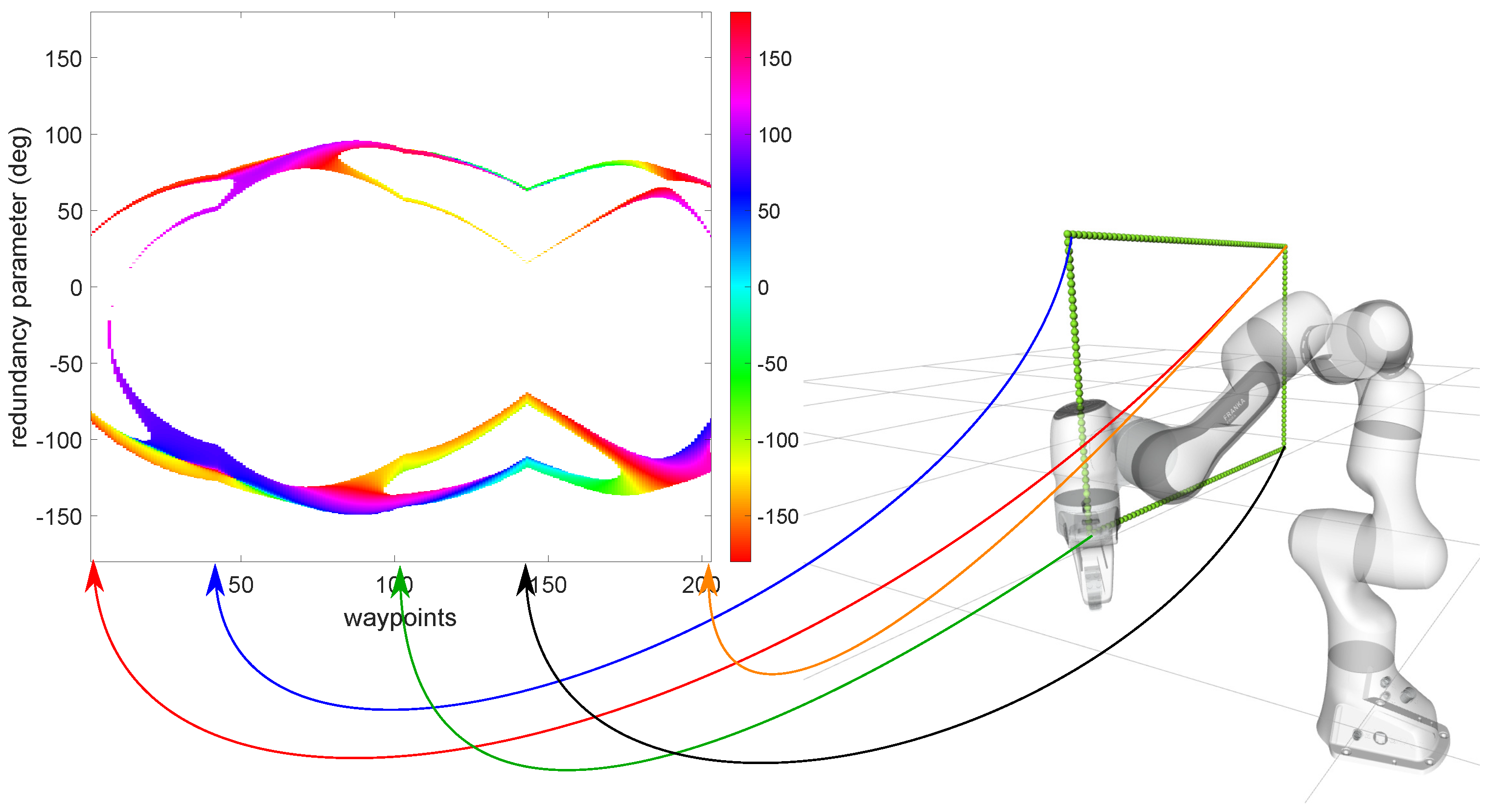
with and . A pictorial view of this process is given in Figure 1 for the case (one degree of redundancy, i.e., ): each column in the grid corresponds to a waypoint on the path and the nodes in a column span the self-motion manifold(s) lying in the null-space. Grids combine self-motions with path tracking and are, therefore, the pre-image of the workspace path in the configuration space.
The “augmented” kinematic function in (9), also termed node function, is equivalent to a standard inverse kinematic function of a non-redundant manipulator, meaning that is not unique, but a finite set of solutions exists. The number of such solutions only depends on the mechanical characteristics of the manipulator and is equal to 2, 2, 4 and 16 for planar, spherical, regional and spatial manipulators respectively [17,18]. However, for some specific kinematic structures, as well as for some specific trajectories [19], the actual number of solutions could be less than the maximum theoretical value. For instance, for most six-axis industrial manipulators, the number of distinct configurations is equal to 8 [11]. Multiple inverse kinematic solutions imply the existence of multiple grids. Therefore, let us rewrite Equation (9) to make the grid index g explicit:
All the inverse kinematic solutions along the assigned path can be classified so as to ensure continuity for each single grid, determining a continuous posture set. For a redundant planar manipulator with Denavit-Hartenberg reference frames, such a classification reduces to testing the sign of the “elbow” joint, so that one grid represents the elbow-down configurations and the other the elbow-up ones. If the kinematic chain is made of many joints, identifying the elbow could be not immediate. Indeed, the elbow itself depends on the chosen redundancy parameter: it will be the joint variable nullifying the extended (or augmented) Jacobian’s determinant; its sign will mark the separation between elbow-down and elbow-up inverse kinematic solutions [14]. In general, if the redundancy parameter changes, the extended Jacobian changes too, and the joint variable nullifying its determinant could be different, as well as the criterion to distinguish between continuous posture sets. For a generic redundant manipulator, the extended Jacobian determinant could be made of several factors. From the topological point of view, all the solutions determining the same signs for such factors are said to belong to the same extended aspect [20] and constitute a continuous posture set. If a grid contains solutions from one and only one extended aspect, it is said to be homogeneous [14]. This concept will be useful in the discussion that follows in Section 2.3.
As a concluding remark on state space grids, it is important to highlight that, although an extended Jacobian is virtually defined once the redundancy parameter is selected, it is never used for kinematic inversion. In agreement with (10), inverse kinematics is always positional, so that the optimization is immune to singularities and algorithmic singularities. As will be clarified next, transitions through singularities are nominal in a discrete dynamic programming approach and, indeed, this is a relevant advantage of this technique over others, including calculus of variations.
2.3. DP-Inspired Search Algorithm
If all the states by which the manipulator can transit are available in the grids, the optimization problem reduces to the selection of the nodes that provide the minimum cost. In this case, the problem is equivalent to that of finding the optimal path on an acyclic directed graph [11], which means that an optimal solution can be found regardless of the Bellman optimality principle, which would rather be necessary if the state set was continuous. Thus, we keep the problem decomposition typical of dynamic programming, where the local optimization problem is simply a node selection problem, which is typical of search algorithms on trees and graphs [21]. With this formulation, several implementations are possible. For instance, we proposed a forward (i.e., from the first waypoint to the last) iterative implementation [14], but alternatives exist to proceed backward (i.e., from the last waypoint to the first) and/or using recursive approaches. It has to be noted that if a forward implementation was chosen, Equation (6) should be rewritten as
In this case it is convenient to redefine as:
and as:
The choice between forward and backward implementation is not, in general, arbitrary, as it often depends on considerations about performance and on the hardware architecture used, as well as on the boundary conditions of the problem.
To better understand how boundary conditions affect the choice, we could highlight that the optimal cost function (backward) or (forward) are conditioned by the sequence of inputs enabled at each i. In many practical cases, unless the environment in which the robot moves is particularly constrained, applications require that either the initial joint positions or the final ones or both are assigned or otherwise constrained (e.g., cyclic joint trajectories). The optimal solution and the value of the cost function will then vary together with the initial or final set of inputs. So we may write as a function of such sets [4], having or .
Assume to run our forward dynamic programming algorithm once, starting with inputs in and ending with inputs in . One execution of the algorithm is sufficient to provide the solution together with its cost for the optimal joint-space paths ending in each single element of . From the practical standpoint, the upside is that one may decide to select a sub-optimal solution if its cost does not vary too much from the optimal cost, while the final joint positions are much more favorable for the particular task the robot has to execute.
On the other hand, if one asked for a solution starting from a specific , this may require an additional execution of the algorithm, either proceeding backward or by explicitly forcing the initial condition at the moment is defined. In other words, one execution of the forward algorithm with free initial conditions does not guarantee the computation of a solution for each input in , as well as one execution of the backward algorithm with free final conditions does not guarantee the computation of a solution for each input in .
Considering the grid representation of Section 2.2, and assuming a forward implementation, we may rewrite Equation (11) as
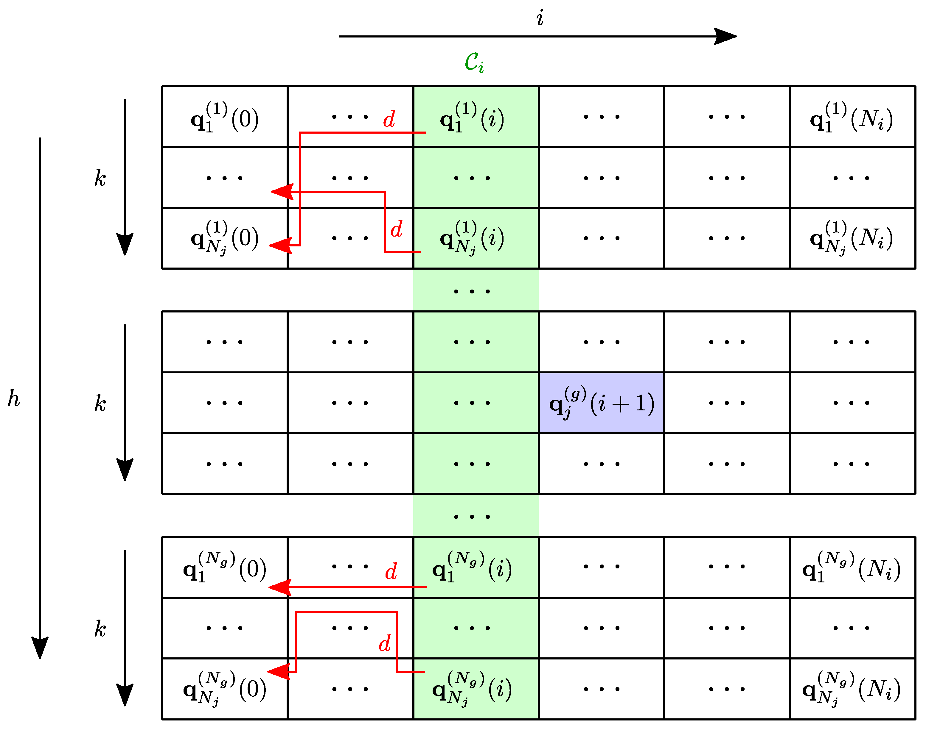
where is the local cost to move from node on grid h to the node on grid g, while is the maximum order derivative for which a constraint is defined; for instance, if acceleration constraints are imposed, . A pictorial view is given in Figure 2 for . For each enabled node at (in blue), an optimal predecessor is selected among those that belong to (in green) by solving the local optimization problem in (14). Higher-order constraints yielding are checked by using the chain of d predecessors represented by the red arrows, which allows computing the discrete approximations of derivatives.
In case Pareto-optimal solutions have to be found, the cost comparison cannot be performed, for each pair of nodes at subsequent stages, on the basis of a scalar cost function. The minimization in (14) is replaced by the dominance rule [4]. Said z the number of performance indices in the Pareto-optimal setup, an objective vector is Pareto-optimal if there does not exist another objective vector such that and for at least one index j. This definition allows defining the dominance rule: given two nodes and , for which the cumulative cost is computed in transiting towards the same node , is said to dominate if improves the vectorial cost function of for at least one performance index, without worsening the others. As a consequence, the optimal predecessor of a given node at i is not a single node at (the predecessor is not unique), as each node might improve the objective vector in a different direction. Every time a dominating node is identified, it enters the list of the optimal predecessors of and the dominated nodes are removed from the same list. As for the scalar objective case, the process is repeated for each i and .
With respect to previous implementations, our algorithms [9,14] provide the evidence that the resolution-optimal solution can be achieved by applying (14) onto all the grids at the same time, i.e., exploring the whole configuration space, and transiting between such grids when necessary, through singularities or semi-singularities of the kinematic chain, using configurations from different extended aspects. They differ in that the former does not make any specific assumption on the homogeneity of the grids, while the latter assumes to work with homogeneous grids to reduce the computational complexity. Both algorithms adopt a forward iterative implementation since, in practical situations, it is more convenient to compute an optimal solution for each single final configuration, starting from one initial configuration, corresponding to the current state of the system. In this communication, we do not make any prior assumption on the grids [9]. However, if we can ensure or detect that grids are homogeneous, we can exploit this information to speed up the search [14].
The computational complexity of the algorithm [9], assuming that the same number of samples is chosen for all the redundancy parameters, is . This is due to the fact that for each waypoint ( waypoints overall) and for each node in the grids ( nodes for each waypoint), a comparison shall be made with each node at the next waypoint ( overall). If the grids are homogeneous, transition points (i.e., nodes corresponding to singularities or semi-singularities where the transition between grids/extended aspects is possible) are clearly identified and the comparisons with the nodes at the next waypoint are only performed within the same grid, lowering the computational complexity to . For a given manipulator, is constant, regardless of the trajectory and, in general, . Thus, the computational complexity can be approximated, in most of the cases, to . Also, homogeneous grids are characterized by continuity of solutions, meaning that, if a certain node does not satisfy the velocity constraints, a farther node will not satisfy them either: this is the assumption at the basis of our optimization [14]. In other words, the velocity constraints allow reducing the number of comparisons for each couple of waypoints to a limited window of nodes, whose cardinality is , with . Therefore, the computational complexity reduces to .
Since all the nodes satisfying the constraints are tested to find the optimum at each stage, resolution-optimality is guaranteed even though the problem in (14) is not convex. Indeed, our method is based on the Bellman optimality principle, ensuring that the solution of the lowest cost is returned for a given discretization of the state space. The compliance of our method to the necessary conditions of calculus of variations has been verified in [9], for a much simpler use case (a planar robot), for which a formulation based on calculus of variations can be obtained straightforwardly.
While this approach might sound demanding in terms of CPU time and memory occupancy, the results of the computational complexity analysis, as well as the specific topological features of spatial robots subject to real-world constraints suggest that solving problem (14) is doable within a time horizon that is compatible with the off-line planning applications mentioned in Section 1. This is shown in Section 4 with an example.
3. ROS Implementation
3.1. Designing an Extension for MoveIt!
MoveIt! [22] is the planning framework of ROS, including several libraries for motion planning, manipulation, 3D perception, kinematics, control and navigation. To the purpose of extending it to perform resolution-optimal inverse kinematics along a specified workspace trajectory, we focus on the analysis of three concepts of interest, which are capabilities, planners and inverse kinematics.
For a robotic manipulator, the MoveIt! user can plan joint-space trajectories and perform several other actions through capabilities, exposed by the move_group node. For instance, the MoveGroupCartesianPathService is used to plan Cartesian paths (straight lines) passing by pre-defined waypoints, the MoveGroupPlanService performs the point-to-point trajectory planning in the joint space, the MoveGroupKinematicsService computes direct and inverse kinematics, and so on.
Except for the MoveGroupCartesianPathService, the move_group node does not allow for any other form of planning in the joint space along a constrained end-effector trajectory. MoveIt! provides several planners, such as OMPL and STOMP [23], just to mention some, which are typically employed in a point-to-point planning scenario, i.e., move the end-effector to a new location along an arbitrary path. Additional constraints can be specified in the Motion Plan Request [24] for any link in the kinematic chain, including the end-effector, but planning for complex paths may not be straightforward and just a few possibilities exist to tune the process to work with generic (possibly multiple) objective functions and application-specific constraints. As far as the MoveGroupCartesianPathService is concerned, the user defines the workspace waypoints, then the end-effector trajectory is simply calculated by first order interpolation. The joint-space planning consists of computing the inverse kinematics for each single waypoint in the interpolated set, but, for a redundant manipulator, no mean exists to control the optimality of the solutions in the joint space along the whole trajectory.
On the other hand, since the dynamic programming algorithm presented in Section 2 is no more than a resolution-optimal inverse kinematic procedure, we may think to extend the inverse kinematics capabilities of MoveIt!. Nonetheless, the resolution-optimal planning is defined on a pre-defined set of waypoints, so that the objective function and constraints can regard the derivatives of the joint position variables, which will depend on the time law defined at the end-effector.
The algorithm we aim to extend MoveIt! with is a planner in that it computes a joint-space trajectory from infinite possible solutions, but, at the same time, it is an IK solver, as it works with an assigned workspace trajectory. Because resolution-optimal inverse kinematics is different from other capabilities of the framework, we believe that providing the functionality as a new move_group capability is the most seamless solution.
3.2. Requirements
On the basis of the considerations above, let us consider the following requirements for our extensions:
- Req. 1:
- to allow for a seamless integration with the ROS ecosystem, so as to reuse, as much as possible, the available technologies (e.g., visualization and analysis tools);
- Req. 2:
- to support the generation of multiple homogeneous grids;
- Req. 3:
- to perform a search on such grids to find the resolution-optimal joint-space solution [9];
- Req. 4:
- to support the optimization for homogeneous grids [14];
- Req. 5:
- to allow for the addition of user-defined constraints and objective functions;
- Req. 6:
- to allow for the topological analysis of the state space and the resolution-optimal trajectory.
3.3. Context
Our moveit_dp_redundancy_resolution package, publicly available on the Internet [25], constitutes an additional move_group capability, which is offered to the MoveIt! users through a ros::ServiceServer. Specific messages, called GetOptimizedJointsTrajectory, are exchanged through the service interface. The user can be any ROS node that implements a ros::ServiceClient interface and is able to assembly and send a GetOptimizedJointsTrajectoryRequest.
To exploit, as much as possible, the available visualization and analysis tools, i.e., Req. 1:, the results of the computation performed by the resolution-optimal planner are published through ros::Publisher objects on specific pre-existing topics, so that other nodes from the ROS ecosystem, such as RViz and rqt_multiplot, can be used to animate the robot along the assigned trajectory and to plot the resulting joint position, velocity and acceleration curves respectively.
Furthermore, in order to satisfy Req. 6:, several functions are provided to export the data structures of interest to the filesystem, to be later imported by additional analysis tools, such as MATLAB functions/scripts or replayed through ROS bagfiles.
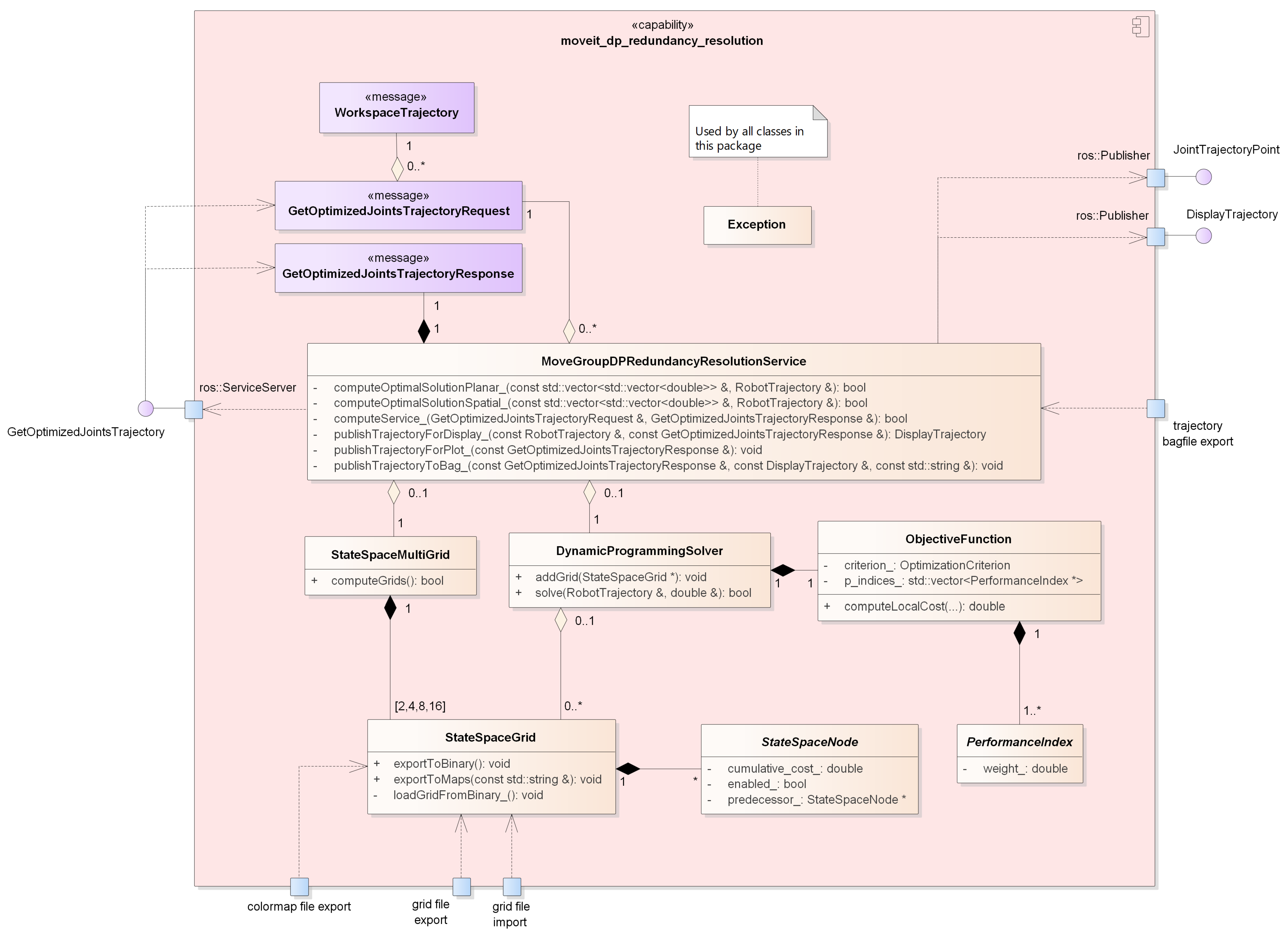
The moveit_dp_redundancy_resolution context is reported in Figure 3, where the extensions are drawn in red. Together with the main ROS developments, additional analysis functions have been developed in MATLAB to perform the off-line topological analysis of both the state space and the resulting resolution-optimal joint-space trajectory. State space grids are exported to custom binary formats, while optimal trajectories are exported to bagfiles and imported in MATLAB through the rosbag interface.
3.4. Architectural Design
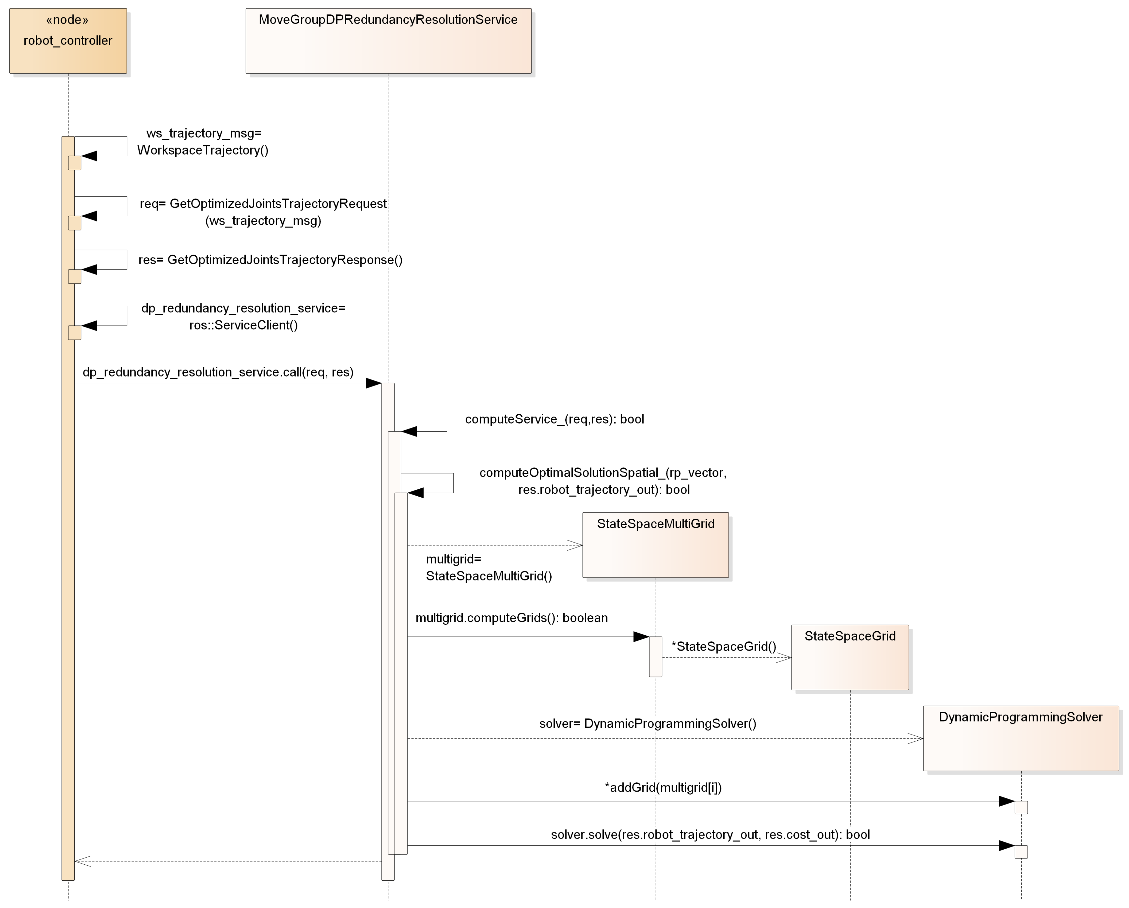
Internally, the ros::ServiceServer is hosted in the MoveGroupDPRedundancyResolutionService class, which constitutes the capability plugin. It is in charge of receiving requests, calling the lower level functions, building up responses and disseminating them through publishers, as well as generating bagfiles. It is instantiated at run-time, depending on the configured move_group capabilities and usually stands next to other default capabilities, as mentioned in Section 3.1. Its client counterpart, the robot_controller node, can call its service or other move_group capabilities, covering a broad range of planning scenarios. For example, one may request a point-to-point planning to OMPL and then use the generated workspace trajectory to issue a resolution-optimal redundancy resolution request. The same could be done with a workspace trajectory generated with the MoveGroupCartesianPathService capability, as will be shown in Section 4.
Behind the MoveGroupDPRedundancyResolutionService, several other objects interact to satisfy the requirements of Section 3.2. In particular, the StateSpaceGrid is the class implementing the data structure representing the joint space along the assigned trajectory. It provides import/export functions for the grid’s custom binary file format as well as the generation of colormaps in the form of raster images that can be directly interpreted by the human user for quicklook purposes. To deal with homogeneous grids, state space grids cannot be generated independently, as it is necessary that the multiple IK solutions are classified per extended aspect, as observed in Section 2.2. For this reason, multiple grids are created by a single execution of the IK solver, supervised by a StateSpaceMultiGrid object. Its primary objective is to control the non-redundant IK solver implementing (10) and to classify the solutions, so as to satisfy Req. 2:.
To speed up the calculation of the state space grids, it is convenient to adopt an analytic inverse kinematic solver that is several orders of magnitude faster than numeric solvers. In the ROS framework, a possibility is given by IKFast, which can find all the IK solutions on the order of 6 microseconds, while most numeric solvers may require even 10 milliseconds or longer, and convergence is not certain [26]. IKFast performs an off-line analytic kinematic inversion and generates a C++ library containing the algebraic IK solver, able to return all the solutions for given end-effector pose. The off-line process may require several minutes, but is independent from the assigned trajectory and, thus, needs to be executed only once for a given kinematic chain. Currently, IKFast is able to manage open kinematic chains with one degree of redundancy. The value of the redundancy parameter has to be provided at the time the algebraic solver is called, which is the case of the DP grids considered in this communication. Nonetheless, it is worth observing that, in this context, it is not necessary that the IK solver natively supports redundant inverse kinematics, as the redundancy parameters are given for each single grid node and the inverse kinematics always involve a non-redundant kinematic chain. This means that our solution is scalable with respect to an arbitrary redundancy degree and IKFast can always be used, provided a suitable definition of the redundant (i.e., including the redundant joints) and non-redundant (i.e., excluding the redundant joints) planning groups.
The equations in (14) are implemented by the DynamicProgrammingSolver class, supporting multi-grid search, thereby satisfying Req. 3:. Since state space grids are added to the solver one by one, specific posture sets can be excluded by not passing them to the solver. To satisfy Req. 4:, the optimization can be explicitly enabled/disabled, depending on whether homogeneous grids can be obtained.
The moveit_dp_redundancy_resolution package provides two extension points, which are the abstract classes PerformanceIndex and StateSpaceNode. The former allows for the definition, through a specific XML-based language, of custom performance indices that can be combined together in an ObjectiveFunction. This is done offline, through configuration files. Optionally, performance indices can be characterized by a weight, used for weighted optimization. Otherwise, they are inserted in a vector and the solution will be Pareto-optimal (in a discrete sense, as discussed above). On the other hand, the StateSpaceNode class allows for the definition of application-specific semantics (even beyond resolution-optimal inverse kinematics) and related constraints. For instance, one may think of using the same classes for time-optimal planning along specified paths, provided that a specific StateSpaceNode implementation is given. These two classes allow satisfying Req. 5:.
3.5. Use of Numeric Solvers
IKFast is characterized by the nice property of returning all the IK solutions in a single call to the solver. Furthermore, under certain circumstances, such solutions could be returned in the same order with respect to the extended aspects. When this happens, no post-processing is required on the IK solutions to generate homogeneous grids. Otherwise, either an explicit analytic factorization of the Jacobian is available, or numeric techniques are employed in order to ensure continuity in the state space.
If an analytic solution cannot be computed at all, or is hard to obtain, numeric solvers can be used instead. They are characterized by the property of returning one or no solution for each single call to the solver and their processing is notoriously time-consuming. To still have some control on the execution time, it is extremely important that the conditions characterizing the extended aspects are known beforehand, so that the search space of the solver can be drastically reduced. If this is not the case, the employment of numeric solvers practically rules out the usage of dynamic programming, as multiple IK searches do not guarantee the achievement of solutions in different extended aspects, but, worse, the same solution may be returned multiple times, making inverse kinematics a time-consuming try-and-error process.
In our implementation, we also provide the possibility of using the numeric solver KDL [27], but with planar manipulators only, where we know the condition separating the (two) extended aspects. This capability is transparently provided by the MoveGroupDPRedundancyResolutionService class. In our experience, for more complex cases where the Jacobian’s factorization is not available, the grids generation time becomes much greater than the time needed for the DP search itself and, consequently, the algorithm becomes unusable in any case of practical relevance.
4. Results
4.1. Use Case Description
To demonstrate that the methodology developed in the previous sections can be effectively applied to a real scenario, let us consider a real robotic arm with 7 degrees of freedom, to which a task constrained in position and orientation is assigned, with a time law. In a first trial, the objective is to reduce the energy consumption indirectly through the minimization of the square norm of joint velocities. Sub-optimal solutions are not of interest, hence the globally optimal one must be found. In a second trial, while minimizing the energy consumption as before, in a Pareto-optimal setup, the distance between the elbow (corresponding to the fourth joint) and an obstacle in the workspace is maximized so as to find a collision-free joint-space trajectory. Since the Panda robot by Franka Emika [29] has 7 degrees of freedom and is the flagship robot of MoveIt!, it is a convenient choice for the experiment at hand.
The modified Denavit-Hartenberg parameters [30] of the Panda robot [31] are reported in Table 1. Let us set the joint position, velocity and acceleration limits according to the datasheet. Limits on the jerk are not considered, but, as noticed by Gao et al. [5], they contribute to generating smoother solutions, which is necessary in all the cases where the resulting trajectory has to be executed on real hardware.
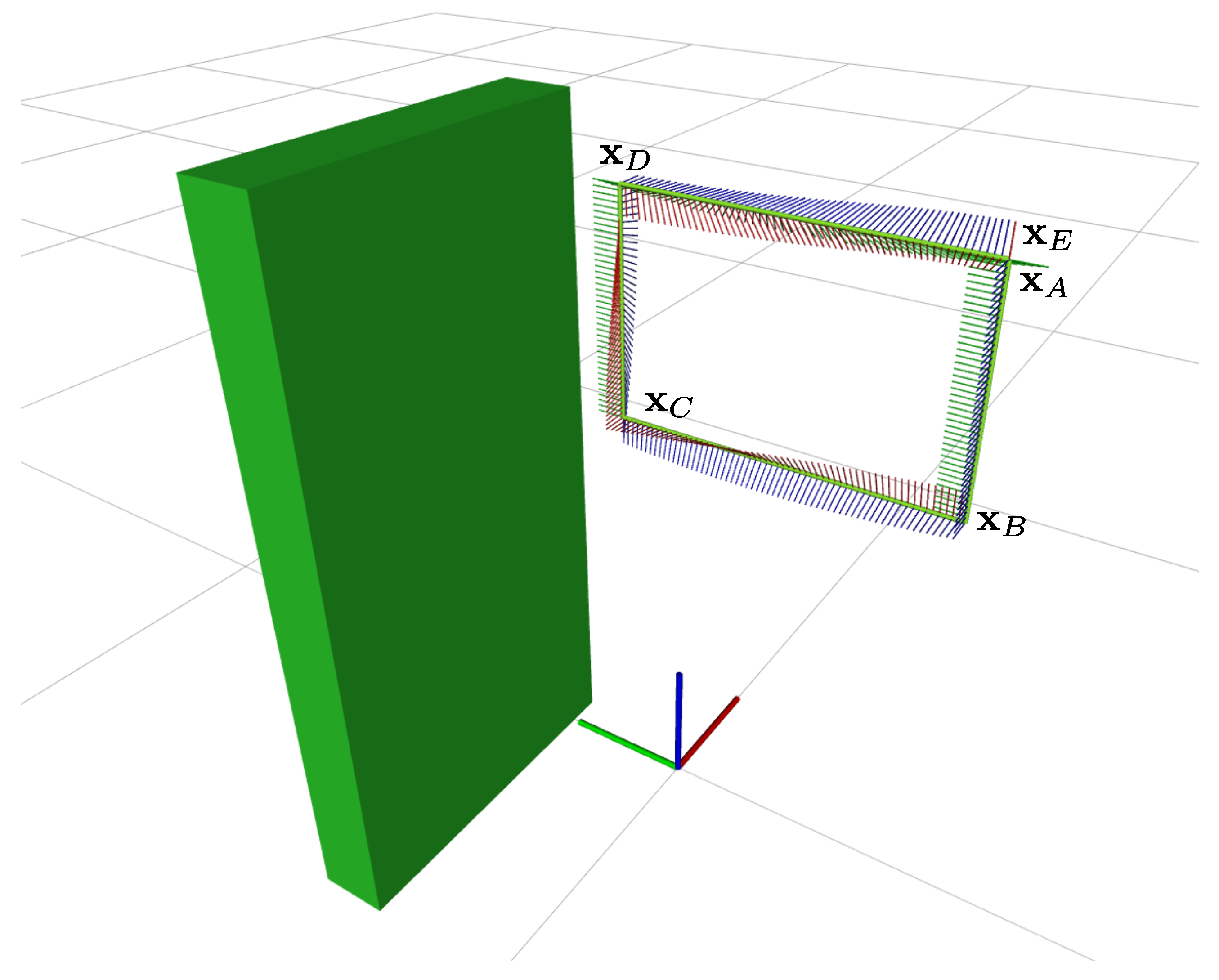
The workspace path is defined in terms of position and orientation and is depicted in Figure 6, together with the base reference frame and the obstacle. The axes x, y and z are in red, green and blue respectively. The planning is performed for the end-effector’s flange that has to visit five waypoints, in the order , , , and , describing the corners of a rectangle in the y-z plane, with variable orientation. Their values with respect to the base reference frame, considering a roll-pitch-yaw representation for the orientation, are
All the points in between each pair of waypoints are obtained by linear interpolation, with a linear resolution not exceeding 0.01 m. A time law is defined so as to complete the whole trajectory in 60 s, with a constant time offset between consecutive points. The total number of points is .
4.2. Grids Computation
As mentioned above in Section 3.4, grids are computed through the StateSpaceMultiGrid class, making use of the IKFast kinematic plugin. The plugin is based on a C++ solver generated off-line, which requires to select a redundant joint with respect to which inverse kinematics expressions are computed. In general, the choice of the redundancy parameter is not arbitrary, for two reasons:
- when fixing the redundant joints to specific values, the manipulator must be no longer redundant in order for (10) to return a finite number of solutions: at algorithmic singularities, i.e., configurations nullifying the determinant of the extended Jacobian, this is not the case.
Both issues are beyond the scope of this paper, but we note that solutions exist to select redundant joints in view of performing inverse kinematics, as well as correctly representing internal motions [32]. In our case, we can obtain an IKFast solver by selecting the redundancy parameter . In fact, since joint 4 is in the middle of the kinematic chain and its axis does not intersect any other joint axis, we minimize the chances of encountering degenerate cases and of handling more complicated expressions [26]. A posteriori, we verify that the selected parameter is representative of the internal motion for the assigned path, i.e., state space grids do not degenerate to lines.
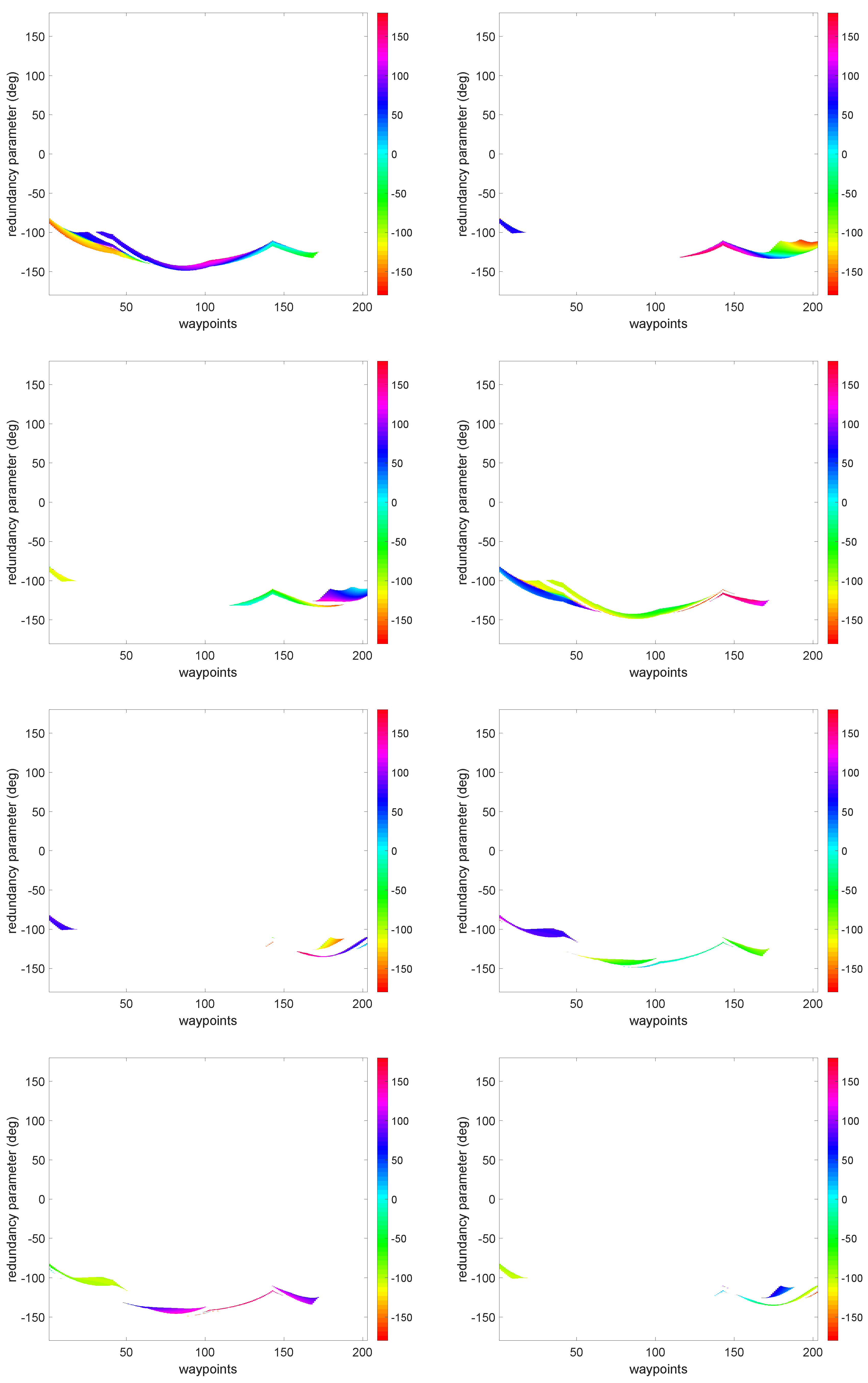
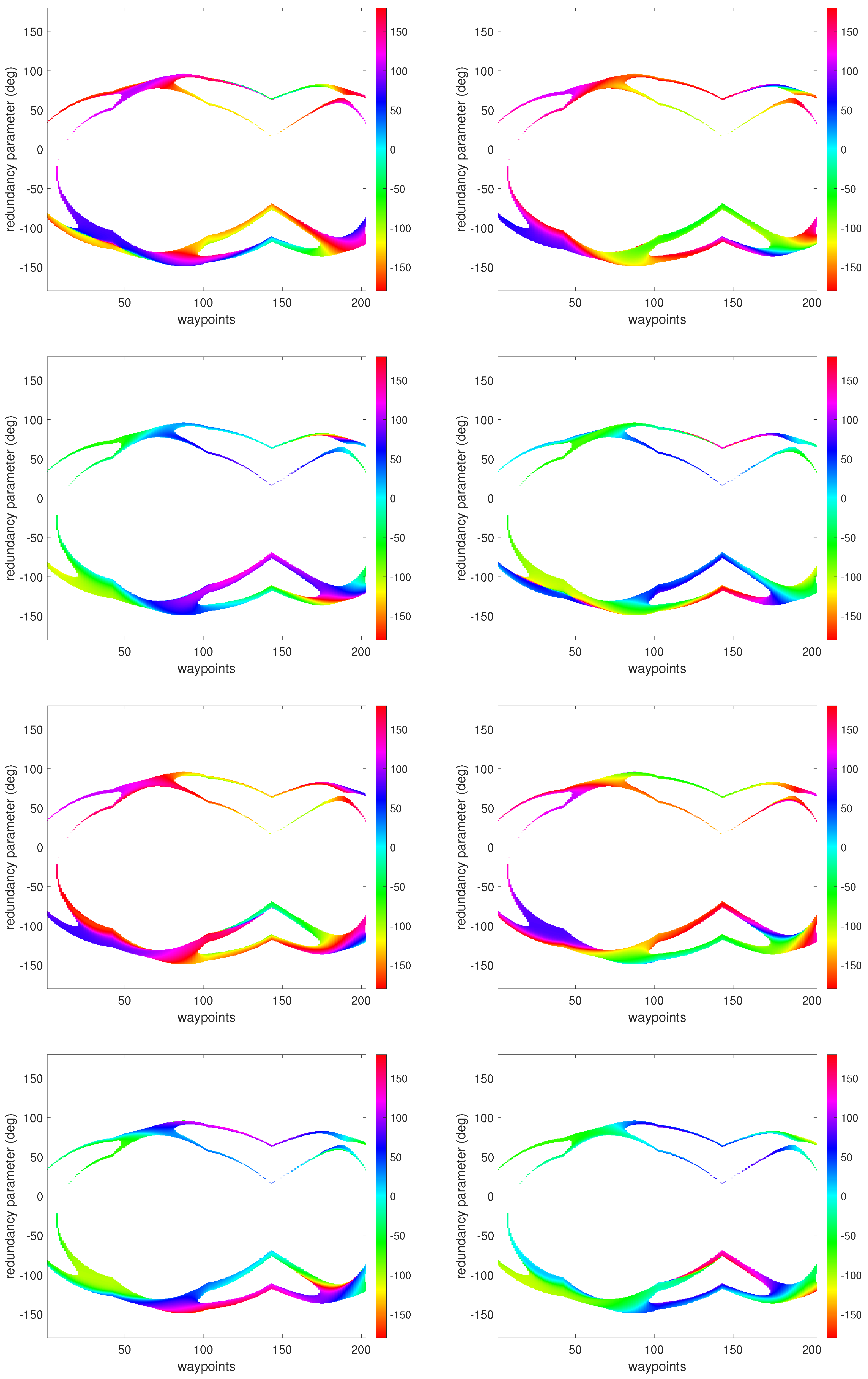
The redundancy parameter can be discretized so that , either between deg and 180 deg, which yields a resolution of deg, or between its physical limits, i.e., deg and deg, which yields a resolution of about deg. The Panda manipulator has 8 IK solutions, i.e., , for all the points on the trajectory, but in practice, because of joint limits, some points have less. The “slices” corresponding to of the grids computed with IKFast are reported in Figure 7, while those computed neglecting joint limits, for comparison purposes, are reported in Figure 8.
The first interesting thing to notice about these grids is that they are homogeneous, as evident from those of Figure 8. The extended Jacobian , obtained from the rectangular Jacobian by adding the row , cannot be easily factorized, implying that we are not provided with analytic conditions to classify the solutions of IKFast. For this reason, the following three conditions are used, obtained from an a-posteriori numerical analysis of the solution sets:
- ;
- ;
- .
Each of the grids in Figure 7 and Figure 8 corresponds to a different combination of the conditions above, providing an homogeneous classification of the solutions. It is possible to demonstrate that both and are factors of and, being the “augmented” Panda manipulator of type 1, according to Wenger [19], they are sufficient conditions for classifying the solutions.
The second trait of interest is that there might exist redundancy parameters other than that are more representative of the internal motion, for the trajectory assigned. In fact, by looking at the grids of Figure 8 (without joint limits), a large portion of the joint domain does not contain any solution. This means that large variations of the other joints shall be expected for little variations of the redundancy parameter: a fine discretization of the redundancy parameter is needed for the dynamic programming algorithm to provide a smooth solution. We recall that, in our case, the selection of is unavoidable for IKFast to produce an anlytical IK solver.
Lastly, it is worth noting that joint limits, in real scenarios, notably reduce the search space, giving a chance to the dynamic programming algorithm to find the resolution-optimal solution in a short time. Also, because of joint limits, the Panda is not able to track the assigned trajectory remaining in the same extended aspect, as none of the grids admits a feasible joint-space path from (corresponding to ) to (corresponding to ). Hence, the robot will need to reconfigure its posture on the way by passing through singularities of its kinematic subchains.
4.3. Globally Optimal and Pareto-Optimal Solution
Since grids are homogeneous, the search can be optimized. Thus, both our algorithms [9,14] can be executed to find the resolution-optimal solution on the grids of Figure 7. Table 2 reports the execution time of both algorithms and different discretization steps of the redundancy parameter, together with the associated cost function, for the case where only energy minimization is considered. Tests have been executed on a 64-bit Ubuntu 16.04 LTS OS running on an Intel® CoreTM i7-2600K CPU @ 3.40GHz × 8. No multi-core execution model has been used in the tests.
It is interesting to notice that there is not any considerable improvement in the performance by using the optimized algorithm in place of the unoptimized algorithm. This means that either position or acceleration limits are almost everywhere stricter than velocity limits for the assigned trajectory. This is in contrast to the use cases where the existence of much less unfeasible cells (i.e., white regions) allows velocity constraints activate first [14].
The convergence rate that we may estimate from the values of the cost function, compared to our previous use case [14], is a confirmation that is very sensitive for the considered trajectory, meaning that small variations of yield considerable changes in the solution for the other joints and, as consequence, in the final value of the cost function.
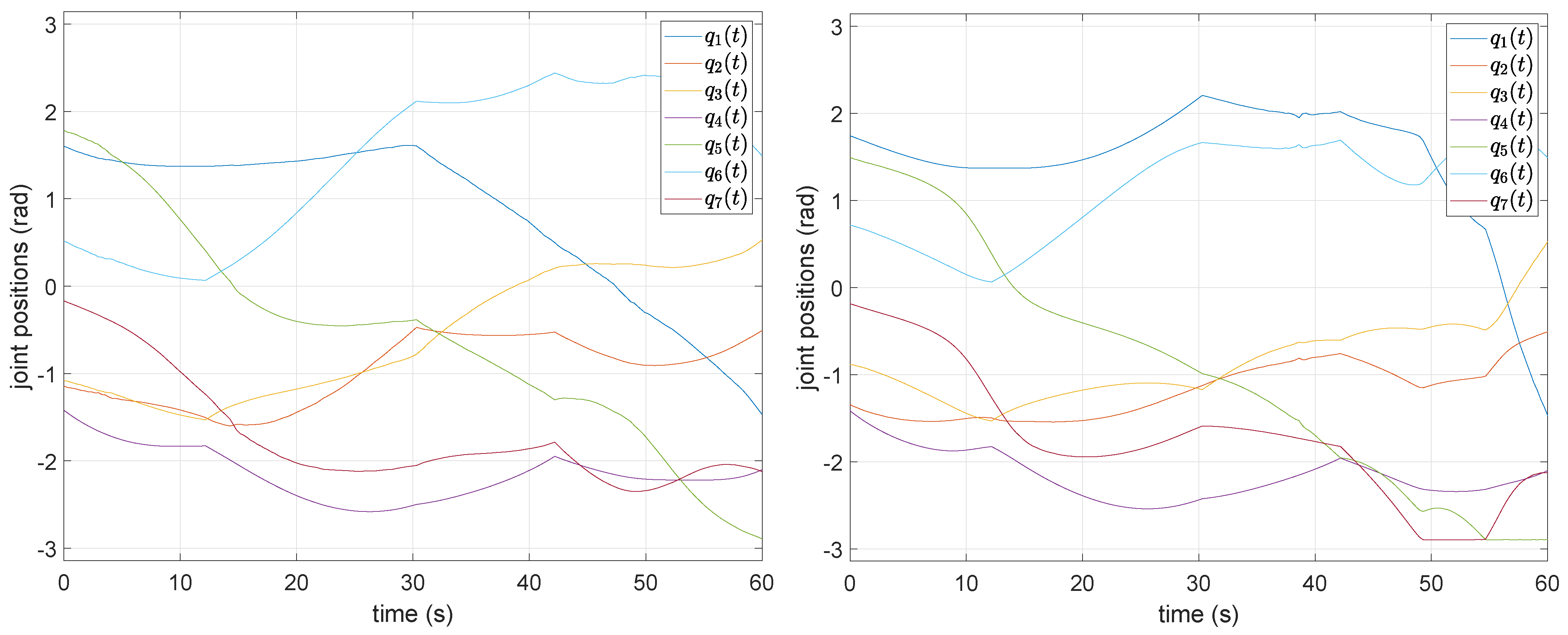
The solution obtained for is reported in Figure 9 (left). It starts from grid 5 (i.e., , , ), then, at s (), it jumps to grid 6 (i.e., , , ) and, at s (), to grid 1 (i.e., , , ). For the majority of the trajectory, up to s (), the solution lies on grid 1. Afterwards, it transits to grid 2 (i.e., , , ) and terminates, achieving 3 posture reconfigurations in total and visiting 4 different extended aspects. As commented in Section 2.3, posture reconfigurations always happen on the boundaries of the feasible (non-white) regions, where two or more of the maps have the same color for all the joints (only is shown in Figure 7). It is easy to verify that this is the case for the sequence of grids visited by the algorithm and transitions at the stages mentioned above.
In the Pareto-optimal setup, in order to provide the solver with a unique optimization criterion (minimization or maximization), the distance from the obstacle is maximized by minimizing the distance between joint 4 and the point , lying on the opposite side with respect to the robot, with the effect of “pulling” it away from the obstacle. Among the solutions in the Pareto set, we select the one that minimizes the norm of the objective vector. For , the cost is , corresponding to square norm of velocities and distance from respectively, while the joint-space solution is shown in Figure 9 (right). As shown in the video [33], the dynamic programming algorithm achieves the computation of an obstacle-free trajectory, while the robot collides if only the square norm of velocities is minimized.
As far as the solutions of Figure 9 are concerned, the reader may clearly notice the discontinuities in the derivative of the joint positions at each of the three intermediate corners of the trajectory. In between these points the curves are not everywhere smooth. As commented by Gao et al. [5], either a post-processing step or the introduction of jerk constraints would be desirable to allow for the execution on real hardware.
5. Discussion
With respect to previous works using a similar DP-based problem formulation, we focused on the design of a maintainable, re-usable, modular and flexible ROS extension that can be generic enough to be employed in a broad range of applications. We provided clear extension points to adapt the software to specific scenarios and introduce custom requirements, such as specific constraints and objective functions. Our solution foresees the development of a minimal amount of code to introduce such modifications, because, when possible, they are enforced through configuration files.
The whole extension is provided in the form of a new move_group capability, meaning that the already existing interfaces are reused as much as possible, so that the user can benefit from already available analysis and visualization tools. Also, we implemented several file export functions, relying as much as possible on existing formats, e.g., bagfiles, so that further tools can be developed even in environments outside of ROS, such as MATLAB.
We emphasized the capability of our algorithm of exploring multiple grids at the same time, which was not evident in previous works, thus ensuring the achievement of the resolution-optimal solution. In our treatment, we did not renounce to the topological analysis of both the manipulator’s null space along the trajectory and the resulting reslution-optimal joint-space solution. Although this is more complicated for spatial manipulators than planar ones, some key features of the problem can be highlighted, as the feasibility of the task and the necessity of traversing singularities or semi-singularities to complete it. Attention was paid to the computational complexity and, in fact, we extended previous algorithms [9,14] to be applied to real robots and demonstrated that, depending on the chosen redundancy parameter and joint limits, not necessarily homogeneous grids yield lower computation times. However, on the other hand, we showed that for real manipulators, dynamic programming is perfectly suited for redundancy resolution as the constraints characterizing real applications drastically reduce the search space and yield a fast convergence.
In our implementation, inverse kinematics plays an important role. First of all, it only concerns position kinematics, thus the robot is free to pass through its singularities as no Jacobian inversion is performed. Second, if an analytic IK solver is available, state space grids can be computed without any knowledge of the extended aspects, and their homogeneity can be imposed numerically. On the contrary, if an analytic solver is not available, and the extended Jacobian cannot be factorized, finding all the possible solutions could be cumbersome, especially in the presence of joint limits. If there is not any certainty that the state space is completely represented, the global optimality of the solution could be affected as well.
Beside possible application-specific extensions, several improvements are possible for our ROS-based implementation. For instance, because the state space is discretized, it might be possible that the solution resulting from the application of the algorithms described in Section 2.3 is not feasible on real hardware. Rather, in other circumstances, it might happen that the trajectory is feasible, but it is not smooth enough to be repeated over and over again without damaging the mechanical parts on the long run. The proposed formulation is straightforward, but, in practice, is not enough to ensure that the motion is always feasible and smooth. In fact, on one hand, the output joint trajectory could exceed joint torque capacities and, on the other, could result in oscillations of the joints because of its non-smoothness. Indeed, while the usage of acceleration constraints allows for smooth joint position functions, it might not be enough to guarantee smoothness at velocity level. In such cases, it might be suitable considering additional constraints on the derivative of the acceleration, which could also be provided in the robots datasheets [5].
Together with the imposed constraints, the discretization step of the redundancy parameter also plays an important role in the generation of smooth joint-space trajectories. It is clear that the finer the discretization is, the smoother the trajectory can be, but this comes to the detriment of time. Indeed, some redundancy parameters have a lower sensitivity with respect to the motion to be performed, meaning that for large changes of their value, all the other variables in play, such as the joint position variables, change less. If this is the case, a coarser discretization can be used for the redundancy parameter, as it is very representative of the motion, resulting in a smooth trajectory, still at a reasonable computation time. Alternatively, an iterative approach can be used, where a finer discretization is performed in the neighborhood of a solution obtained with a coarser discretization at the previous iteration [5]. This technique yields satisfactory results, but may compromise the optimality of the solution if the first discretization is too coarse.
In some other works [10,11], the trajectory smoothness has also been explicitly included in the performance index to optimize. Specific smoothness measures can be suitably combined with other performance indices of interest for the specific application, but the result will always be a sub-optimal solution with respect to each of the indices. Gao et al. [5] consider a different approach, which is based on the post-processing of the solution. In particular, the redundancy parameter curve is smoothened by applying a fifth-order polynomial approximation. Then, in order to guarantee that the trajectory is exactly tracked, inverse kinematics is solved again with the new values of the redundancy parameter.
6. Conclusions
In this paper we proposed a novel architecture to perform redundancy resolution through the global optimization of performance indices, employing a dynamic programming formalism. In particular, the problem formulation foresees the discretization of the state space and its representation in the form of multiple grids. Then, a DP-inspired graph search algorithm is used to ensure the achievement of the resolution-optimal solution.
The developed software components extend the open-source framework ROS, and integrate seamlessly with the existing packages so as to promote the reuse of the available visualization and analysis tools. On the other hand, they provide clear extension points that can be used to introduce user-specific requirements, so that the new capability can be easily adopted in a broad range of applications, with a minimum development effort, even beyond redundancy resolution.
If the underlying state space grids are characterized by continuity, i.e., they are homogeneous, the developed algorithm can exploit this feature to optimize the multi-grid search. This is particularly advantageous when the velocity limits are stricter than other constraints. Moreover, the proposed architecture provides the means to analyze the intermediate and final products of the computation from the topological point of view, and further analysis tools can be developed in MATLAB or other languages.
Nonetheless, our architecture does not guarantee that the resolution-optimal joint-space solution can be directly sent to a real robot controller, although additional constraints and/or processing steps can be defined either through our extension points or the ROS ecosystem.
Future work may concern the introduction of parallel computational models, which would further improve the performance of the algorithm, as well as the extension toward other problems/semantics, such as time-optimal planning along specified paths.
Author Contributions
Conceptualization, E.F. and P.C.; methodology, E.F.; software, E.F. and F.S.; validation, E.F.; investigation, E.F.; resources, F.S. and P.C.; data curation, E.F. and F.S.; writing—original draft preparation, E.F.; writing—review and editing, E.F., F.S. and P.C.; visualization, E.F.; supervision, F.S. and P.C.; project administration, P.C.; funding acquisition, P.C. All authors have read and agreed to the published version of the manuscript.
Funding
This research was partly funded by Italian Ministry of Education, University and Research (MIUR) grant number CUP D49D17000250006. The APC was funded by the University of Salerno.
Institutional Review Board Statement
Not applicable.
Informed Consent Statement
Not applicable.
Data Availability Statement
The source code presented in this study is openly available in GitHub/Zenodo [25], version v0.1.0. More data are available on request from the corresponding author.
Conflicts of Interest
The authors declare no conflict of interest.
References
- Siciliano, B.; Khatib, O. Springer Handbook of Robotics; Springer International Publishing: Berlin/Heidelberg, Germany, 2016. [Google Scholar] [CrossRef]
- Kazerounian, K.; Wang, Z. Global versus local optimization in redundancy resolution of robotic manipulators. Int. J. Robot. Res. 1988, 7, 3–12. [Google Scholar] [CrossRef]
- Nakamura, Y.; Hanafusa, H. Optimal redundancy control of robot manipulators. Int. J. Robot. Res. 1987, 6, 32–42. [Google Scholar] [CrossRef]
- Guigue, A.; Ahmadi, M.; Hayes, M.J.D.; Langlois, R.; Tang, F.C. A dynamic programming approach to redundancy resolution with multiple criteria. In Proceedings of the IEEE International Conference on Robotics and Automation, Rome, Italy, 10–14 April 2007; pp. 1375–1380. [Google Scholar] [CrossRef]
- Gao, J.; Pashkevich, A.; Caro, S. Optimization of the robot and positioner motion in a redundant fiber placement workcell. Mech. Mach. Theory 2017, 114, 170–189. [Google Scholar] [CrossRef]
- Shen, Y.; Huper, K. Optimal trajectory planning of manipulators subject to motion constraints. In Proceedings of the 12th International Conference on Advanced Robotics, Seattle, WA, USA, 17–20 July 2005. [Google Scholar] [CrossRef]
- Ascher, U.M.; Mattheij, R.M.M.; Russell, R.D. Numerical Solution of Boundary Value Problems for Ordinary Differential Equations; Society for Industrial and Applied Mathematics: Philadelphia, PA, USA, 1995. [Google Scholar] [CrossRef]
- Keller, H.B. Numerical Methods for Two-Point Boundary-Value Problems; Courier Dover Publications: Garden City, NY, USA, 2018. [Google Scholar]
- Ferrentino, E.; Chiacchio, P. A topological approach to globally-optimal redundancy resolution with dynamic programming. In ROMANSY 22–Robot Design, Dynamics and Control; Arakelian, V., Wenger, P., Eds.; Springer: Cham, Switzerland, 2018; Volume 584, pp. 77–85. [Google Scholar] [CrossRef]
- Pashkevich, A.P.; Dolgui, A.B.; Chumakov, O.A. Multiobjective optimization of robot motion for laser cutting applications. Int. J. Comput. Integr. Manuf. 2004, 17, 171–183. [Google Scholar] [CrossRef]
- Dolgui, A.; Pashkevich, A. Manipulator motion planning for high-speed robotic laser cutting. Int. J. Prod. Res. 2009, 47, 5691–5715. [Google Scholar] [CrossRef] [Green Version]
- Guigue, A.; Ahmadi, M.; Langlois, R.; Hayes, M.J.D. Pareto optimality and multiobjective trajectory planning for a 7-DOF redundant manipulator. IEEE Trans. Robot. 2010, 26, 1094–1099. [Google Scholar] [CrossRef]
- Cavalcanti Santos, J.; Martins da Silva, M. Redundancy Resolution of Kinematically Redundant Parallel Manipulators Via Differential Dynamic Programing. J. Mech. Robot. 2017, 9. [Google Scholar] [CrossRef]
- Ferrentino, E.; Chiacchio, P. On the optimal resolution of inverse kinematics for redundant manipulators using a topological analysis. J. Mech. Robot. 2020, 12. [Google Scholar] [CrossRef]
- What is ROS? Available online: http://www.ros.org/ (accessed on 3 March 2021).
- Ferrentino, E.; Chiacchio, P. Redundancy parametrization in globally-optimal inverse kinematics. In Advances in Robot Kinematics 2018; Lenarcic, J., Parenti-Castelli, V., Eds.; Springer: Cham, Switzerland, 2018; Volume 8, pp. 47–55. [Google Scholar] [CrossRef]
- Burdick, J.W. On the inverse kinematics of redundant manipulators: Characterization of the self-motion manifolds. In Proceedings of the 4th International Conference on Advanced Robotics, Scottsdale, AZ, USA, 14–19 May 1989; Waldron, K.J., Ed.; Springer: Berlin/Heidelberg, Germany, 1989; Volume 4, pp. 25–34. [Google Scholar] [CrossRef]
- Burdick, J.W. On the Inverse Kinematics of Redundant Manipulators: Characterization of the Self-Motion Manifolds. In Proceedings of the IEEE International Conference on Robotics and Automation, Scottsdale, AZ, USA, 14–19 May 1989; pp. 264–270. [Google Scholar] [CrossRef]
- Wenger, P. A New General Formalism for the Kinematic Analysis of All Nonredundant Manipulators. In Proceedings of the IEEE International Conference on Robotics and Automation, Nice, France, 12–14 May 1992; pp. 442–447. [Google Scholar] [CrossRef]
- Pámanes, J.A.; Wenger, P.; Zapata, J.L. Motion Planning of Redundant Manipulators for Specified Trajectory Tasks; Advances in Robot Kinematics; Springer: Dordrecht, The Netherlands, 2002; pp. 203–212. [Google Scholar] [CrossRef]
- Sniedovich, M. Dijkstra’s algorithm revisited: The dynamic programming connexion. Control. Cybern. 2006, 35, 599–620. [Google Scholar]
- MoveIt. Available online: https://moveit.ros.org/ (accessed on 3 March 2021).
- MoveIt Planners. Available online: https://moveit.ros.org/documentation/planners/ (accessed on 3 March 2021).
- MoveIt Concepts. Available online: https://moveit.ros.org/documentation/concepts/ (accessed on 3 March 2021).
- Ferrentino, E.; Salvioli, F. ROS/MoveIt! Extension for Redundancy Resolution with Dynamic Programming. GitHub/Zenodo. Available online: https://zenodo.org/record/3236880#.YAsFiehKhPY (accessed on 3 March 2021).
- Diankov, R. Automated Construction of Robotic Manipulation Programs. Ph.D. Thesis, Carnegie Mellon University, Pittsburgh, PA, USA, 26 August 2010. Available online: http://www.programmingvision.com/rosen_diankov_thesis.pdf (accessed on 3 March 2021).
- KDL Wiki. Available online: http://www.orocos.org/kdl (accessed on 3 March 2021).
- Ferrentino, E.; Chiacchio, P. Topological analysis of global inverse kinematic solutions for redundant manipulators. In ROMANSY 22–Robot Design, Dynamics and Control; Arakelian, V., Wenger, P., Eds.; Springer: Cham, Switzerland, 2018; Volume 584, pp. 69–76. [Google Scholar] [CrossRef]
- Panda Powertool. Available online: https://www.franka.de/panda (accessed on 3 March 2021).
- Khalil, W.; Kleinfinger, J. A new geometric notation for open and closed-loop robots. In Proceedings of the IEEE International Conference on Robotics and Automation, San Francisco, CA, USA, 7–10 April 1986; pp. 1174–1179. [Google Scholar] [CrossRef]
- Franka Control Interface Documentation. Available online: https://frankaemika.github.io/docs/ (accessed on 3 March 2021).
- Zaplana, I.; Basanez, L. A novel closed-form solution for the inverse kinematics of redundant manipulators through workspace analysis. Mech. Mach. Theory 2018, 121, 829–843. [Google Scholar] [CrossRef] [Green Version]
- Ferrentino, E.; Salvioli, F. Redundancy Resolution for Energy Minimization and Obstacle Avoidance with Franka Emika’s Panda Robot. Available online: https://youtu.be/AxL755_t3_o (accessed on 3 March 2021).
Figure 1.
Mapping of the workspace path in the joint space yielding the state space grids.

Figure 2.
Pictorial representation of the local optimization problem.

Figure 3.
Context diagram.

Figure 4.
Hybrid decomposition/class diagram.

Figure 5.
Sequence diagram representing dynamic programming redundancy resolution.

Figure 6.
Workspace path assigned to the Panda arm, together with the base reference frame and obstacle.
Figure 6.
Workspace path assigned to the Panda arm, together with the base reference frame and obstacle.

Figure 7.
Panda grids (each corresponding to a different extended aspect) representing for the trajectory described in Section 4.1 considering joint limits.
Figure 7.
Panda grids (each corresponding to a different extended aspect) representing for the trajectory described in Section 4.1 considering joint limits.

Figure 8.
Panda grids (each corresponding to a different extended aspect) representing for the trajectory described in Section 4.1 neglecting joint limits.
Figure 8.
Panda grids (each corresponding to a different extended aspect) representing for the trajectory described in Section 4.1 neglecting joint limits.

Figure 9.
Discrete globally optimal (left) and Pareto-optimal (right) solution for the Panda example.
Figure 9.
Discrete globally optimal (left) and Pareto-optimal (right) solution for the Panda example.


Table 1.
Panda modified Denavit-Hartenberg parameters.
| J1 | 0 | 0 | ||
| J2 | 0 | 0 | ||
| J3 | 0 | |||
| J4 | 0 | |||
| J5 | ||||
| J6 | 0 | 0 | ||
| J7 | 0 | |||
| Flange | 0 | 0 | 0 |
Table 2.
Cost function and performance of DP redundancy resolution algorithm for the Panda example, minimizing the square norm of velocities.
Table 2.
Cost function and performance of DP redundancy resolution algorithm for the Panda example, minimizing the square norm of velocities.
| Redundancy Parameter Resolution | Non-Optimized Algorithm [9] | Optimized Algorithm [14] | Cost | |
|---|---|---|---|---|
| 360 | 0.48 deg | 11 s | 11 s | 4.27 |
| 720 | 0.24 deg | 54 s | 54 s | 2.76 |
| 1440 | 0.12 deg | 4 min | 4 min | 2.44 |
| 2880 | 0.06 deg | 14 min | 13 min | 2.16 |
| 4000 | 0.04 deg | 27 min | 26 min | 2.04 |
Publisher’s Note: MDPI stays neutral with regard to jurisdictional claims in published maps and institutional affiliations. |
© 2021 by the authors. Licensee MDPI, Basel, Switzerland. This article is an open access article distributed under the terms and conditions of the Creative Commons Attribution (CC BY) license (http://creativecommons.org/licenses/by/4.0/).
Share and Cite
MDPI and ACS Style
Ferrentino, E.; Salvioli, F.; Chiacchio, P. Globally Optimal Redundancy Resolution with Dynamic Programming for Robot Planning: A ROS Implementation. Robotics 2021, 10, 42. https://0-doi-org.brum.beds.ac.uk/10.3390/robotics10010042
AMA Style
Ferrentino E, Salvioli F, Chiacchio P. Globally Optimal Redundancy Resolution with Dynamic Programming for Robot Planning: A ROS Implementation. Robotics. 2021; 10(1):42. https://0-doi-org.brum.beds.ac.uk/10.3390/robotics10010042
Chicago/Turabian StyleFerrentino, Enrico, Federico Salvioli, and Pasquale Chiacchio. 2021. "Globally Optimal Redundancy Resolution with Dynamic Programming for Robot Planning: A ROS Implementation" Robotics 10, no. 1: 42. https://0-doi-org.brum.beds.ac.uk/10.3390/robotics10010042
Note that from the first issue of 2016, this journal uses article numbers instead of page numbers. See further details here.