Particle Swarm Optimization—An Adaptation for the Control of Robotic Swarms


1
Department of Electronic & Electrical Engineering, University of Bath, Bath BA2 7AY, UK
2
Department of Mechanical Engineering, University of Bath, Bath BA2 7AY, UK
*
Author to whom correspondence should be addressed.
Robotics 2021, 10(2), 58; https://0-doi-org.brum.beds.ac.uk/10.3390/robotics10020058
Submission received: 9 March 2021
/
Revised: 25 March 2021
/
Accepted: 2 April 2021
/
Published: 8 April 2021
(This article belongs to the Section Intelligent Robots and Mechatronics)
Abstract
:Particle Swarm Optimization (PSO) is a numerical optimization technique based on the motion of virtual particles within a multidimensional space. The particles explore the space in an attempt to find minima or maxima to the optimization problem. The motion of the particles is linked, and the overall behavior of the particle swarm is controlled by several parameters. PSO has been proposed as a control strategy for physical swarms of robots that are localizing a source; the robots are analogous to the virtual particles. However, previous attempts to achieve this have shown that there are inherent problems. This paper addresses these problems by introducing a modified version of PSO, as well as introducing new guidelines for parameter selection. The proposed algorithm links the parameters to the velocity and acceleration of each robot, and demonstrates obstacle avoidance. Simulation results from both MATLAB and Gazebo show close agreement and demonstrate that the proposed algorithm is capable of effective control of a robotic swarm and obstacle avoidance.
1. Introduction
Particle Swarm Optimization (PSO) [1] is a popular swarm intelligence algorithm that is used to minimize a cost function (or maximize a fitness function) in a multidimensional space. PSO uses multiple particles, with the velocity of each particle updated based on costs evaluated and shared by the entire swarm. PSO has been used successfully in many different tasks, including artificial neural network training, scheduling problems, and calibration problems [2,3,4,5]. Optimization commonly takes place in a synthetic environment, where virtual particles are allowed to roam without any physical constraints.
The PSO algorithm itself has multiple parameters, and many studies have provided design guidelines for selecting these parameters to ensure both stability and rapid convergence [6,7,8,9,10]. These studies have made several assumptions. The non-stagnant distribution assumption model is so far the closest to completely describing PSO, and the study employing it was able to prove order-1 and order-2 stability of the algorithm [10]. These orders of stability show that over time, both the expected position of a particle and its variance converge to a constant. All the existing analyses study the evolution of the swarm as a whole, and there are no studies of the short-term behavior of each particle.
1.1. PSO in Swarm Robotics
Swarm Robotics is the study of how a swarm of small, simple, and usually identical robots can be used to perform tasks that are not readily performed by a single robot. A swarm robotic system can be characterized by its robustness, flexibility and scalability [11,12]. Swarm robotic systems can be used for many different tasks (e.g., spatial organization, collective motion and decision making [12]). The particle swarms in PSO are analogous to a physical robotic swarm. Therefore, it comes as no surprise that PSO has been proposed as a control strategy for swarm robotic systems [13]. Indeed, several modified PSO algorithms have been proposed for this purpose [14,15,16]. The main focus of these algorithms is to incorporate obstacle avoidance in the movement of the robots. Some other swarm intelligence algorithms that have been proposed for use as swarm controllers in target localization tasks are Glowworm Swarm Optimization (GSO), Artificial Bee Colony Optimization (ABCO), Bacterial Foraging Optimization (BFO), the Firefly algorithm and the Bees algorithm [13].
The use of PSO as a robot controller in swarm robotic systems has the following general problems:
- 1.
- As recognized by Hereford et al [17], the particles in PSO are assumed to be physically unconstrained (i.e., unconstrained velocity and acceleration); an assumption that does not hold for physical robots.
- 2.
- The control of the robots, and the updating of the robots’ states, are performed asynchronously. The rate at which the velocity is updated depends on the speed of robot control system. Therefore, changing the loop delay of a controller will result in different characteristics of the physical system, even if the PSO parameters used remain the same.
The parameter tuning guidelines that are suitable for PSO as applied to numerical parameter optimization are not therefore applicable for swarm robotics applications. Furthermore, PSO when used specifically in source localization tasks, also has the following problems:
- 3.
- PSO assumes an immutable environment. That is because PSO does not consider if the cost (fitness) of past locations might change with time. This is clearly incompatible to real-world robotic applications where both the state of the source and the environment can change.
- 4.
- It is impossible for the swarm to know the location of a source before a particle has passed directly over it, this is incompatible with collision avoidance.
These problems have prevented PSO from being more widely used in swarm robotics. The first problems that need to be addressed are Problems 1 and 2 since they prevent PSO from being used in swarm robotics in general (i.e., they are not limited to source localization). In this paper necessary changes are introduced to the original PSO algorithm to solve these problems. Furthermore, a formalized parameter selection technique is presented that ensures order-1 and order-2 stability of the system, while accommodating the physical constraints (velocity and acceleration limits) of the individual robots. This leads to a new form of PSO with dynamic velocity control and obstacle avoidance that outperforms existing methods. Section 2 provides an introduction to PSO. Section 3 modifies the PSO algorithm for use in swarm robotic systems and develops formalized parameter selection methods. A simulation environment and working example is described in Section 4 and results are given in Section 5.
2. Particle Swarm Optimization Theory
The fundamental aim of PSO is to identify the location inside a multidimensional space that minimizes a cost function by using a swarm of particles. It is also possible to maximize the function, but from this point onwards the assumption will be minimization. At each timestep, every particle calculates the cost of its current location. Each particle stores the location of its lowest cost (personal best location) and communicates it to the rest of the swarm. Therefore, every particle also knows the location with lowest cost of the whole swarm (global best location). After computing and communicating the personal and global best locations each particle updates its velocity based on these values.
Let be the cost function that needs to be minimized, where d is the number of dimensions. Let the particle swarm be a set of N particles located in , at timestep . Each particle computes the cost of its current location using f. The movement of the particles is then determined by the displacement update equation
and the velocity update equation
where and are the velocity and displacement of each particle i at timestep , respectively. The ∘ operator represents element-wise multiplication (i.e., the Schur product). Each element of the vectors and is drawn from the uniform distribution,
The location is the personal best location for particle i, such that for any timestep
Similarly, is the global best location, such that for any particle
The parameters and are the inertia weight, the cognitive coefficient and the social coefficient respectively [10]. The inertia weight prevents the particles of the swarm from diverging uncontrollably from either the personal or global best locations. Larger values of are perceived as allowing more exploration and expansion of the swarm in the problem space. Lower values of are instead used to enable rapid convergence. The cognitive coefficient and social coefficient control the rate of convergence towards a personal best () or global best () location. When , each particle will favor moving towards its personal best location, and when , the global best location [18,19,20].
To simplify further analysis, and in line with assumptions made in previous analyses, will be drawn from a distribution with well-defined mean and variance [9,10]. To follow these previous analyses further, only the behavior of a single particle will be considered, and so the index i will be omitted.
2.1. Parameter Tuning
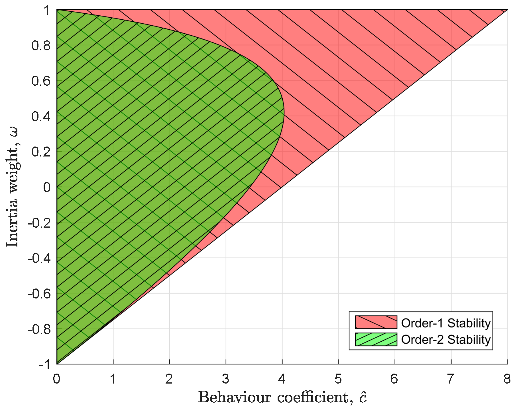
PSO stability analyses typically aim to guarantee order-1 and order-2 stability [10], although higher orders of stability can be also studied [21]. Order-1 is guaranteed by
where is the behavior coefficient and is given by
Order-2 is guaranteed by
These safe operating regions are visualized in Figure 1. The limits ensure convergence towards either of the currently known personal and global best locations [10].
2.2. Introduction to RPSO
Robotic Particle Swarm Optimization (RPSO) is a popular approach that incorporates obstacle avoidance into PSO using an additional acceleration term [14]. Therefore, the velocity update equation becomes
where is the obstacle susceptibility coefficient and each element of is drawn from the uniform distribution . The vector is a virtual force used to push the robot away from surrounding obstacles and it is given by
where P is the total number of obstacles around the robot and is a virtual repulsive force exerted by obstacle . Virtual forces are a well-studied feature in swarm robotics, used to control the position of a robot relative to its direct surroundings (e.g., obstacles or other robots). They are part of the more general Virtual Physics-based Design concept. A number of papers discuss virtual forces and offer different ways of how they can be calculated, ranging from simple position-dependent functions to more complex functions that are typically inspired from real-world physical forces (e.g., spring-dumper systems) [22,23,24,25]. In this paper we make use of simple position-dependent virtual forces to achieve aggregation, but more complex functions should be equally applicable. To define , let be a vector of distances between the robot and surrounding obstacles, such that at the robot has collided with obstacle p. Therefore, a virtual repulsive force is given by
where is the position of the center of the robot, is the position of the center of obstacle p. The parameter is the sensitivity parameter and adjusts the intensity of the repulsive force.
The value of relative to and greatly affects the performance of the algorithm [14]. When , the effect of the last term of (9) may not be sufficient to force the robot to avoid an obstacle. On the other hand, when , the robot becomes overly sensitive to obstacles. Furthermore, all three acceleration terms are unbounded and can increase arbitrarily, leading to further collisions.
2.2.1. Dynamic Velocity Control
Traditionally PSO parameters are tuned before running the algorithm and they remain constant throughout the operation of the algorithm. Couceiro et al. proposed that the value of could be dynamically recalibrated [14]—a form of Dynamic Velocity Control (DVC). When no obstacles are present, tends to 0, but it grows the closer the robot is to an obstacle. However, even if this strategy is employed the unbounded nature of the acceleration terms in (9) can still result in collisions.
For the strategy to work, it must be possible to calculate the maximum velocity that a robot can reach without colliding with an obstacle, and then ensure that this velocity is never exceeded by the RPSO controller. Fortunately, this requirement aligns with the more general problems given in Section 1.1, and they can be solved together by relating the RPSO parameters to the maximum velocity of the robot.
3. Particle Swarm Optimization in Swarm Robotics
3.1. Adaptation of PSO for Swarm Robotics
To formalize the relationship between the PSO parameters and the velocity (and acceleration) of the robot it is necessary to re-state the governing equations. First, a modified form of the update Equation (1) is required,
where represents the discrete timestep (and thus 1/ the update rate) of the PSO controller, which represents the time taken to evaluate a new displacement and velocity vector. Delays caused by inter-robot communication and processing of sensor input will lead to larger values of . The robot may employ other low-level local controllers for tasks that require a higher refresh rate (e.g., motor controllers, data collection and data fusion controllers etc.).
Furthermore, in (2), the terms and are unconstrained, producing what was called Acceleration by Distance by Kennedy [1]. Constraints can be realized by replacing (2) with
The sgn function, which is given by
is also taken from the work of Kennedy (where its use is implied), and limits the maximum acceleration of a single robot by constraining each term of the velocity update equation. Please note that the sgn function is not a smooth function and may result in chattering [26] under certain conditions. A smooth function can be used instead (e.g., tanh or some type of a logistic function with outputs in the range (−1,1)) to avoid this. This paper considers the sgn function for simplicity, but all the results of the following analysis can be applied to the aforementioned smooth functions as well.
3.2. Updated Parameter Tuning Stability Criteria
The stability criteria of (6) and (8) must now be redefined for (13) to ensure stability. Using any of the stability analysis methods mentioned (i.e., [9,10]), the criteria for both order-1 and order-2 stability now become
However, using negative values of would result in the velocity of the robot changing direction at every timestep. Similarly, using negative values for would drive the robots away from the personal and global best locations. Therefore, the criteria of (15) become
3.3. Control of Velocity and Acceleration
An analysis of how the inertia weight and the cognitive coefficient impact on the velocity and acceleration of the robot is now possible. This analysis will consist of three stages: First a state model will be derived in matrix form that describes a robot at each timestep, secondly the state model will be decomposed to understand how the state changes from one timestep to another, and finally expressions for the maximum velocity and acceleration of the robot will be derived in terms of and .
Equation (13) can be simplified based on the stability study of Trelea [7] so that
where is the weighted average of and as shown below
The vector is a random vector of which each component is drawn from the uniform distribution such that
3.3.1. State Model
In control theory, the state of a robot may be described by its position and velocity at a specific timestep. The state vector , which describes the state of motion in each of the d dimensions for a single robot, is given by
where describes the state of motion in only a single dimension j such that
where and are the components of position () and velocity (). PSO algorithms have no interdependency between dimensions, therefore it is possible to use the single-dimension state vector as a general description of every dimension of . Therefore, Equations (12) and (17) can be written in matrix form for each dimension j as
where the right-hand-side consists of a deterministic term and a stochastic term , such that
This is a second order system in terms of position and velocity. However, as the objective is to understand how and will affect velocity and acceleration, acceleration will be included as a state variable. By differentiating (17), the acceleration is given by
The positional stability of PSO has been proven previously, and both the velocity and the acceleration are linearly independent of the position [9,10]. Therefore, for the sake of simplification position will be removed from the state. Thus, a new single-dimension state vector is defined as
Using (17) and (21), the new state model is given by
where the right-hand-side consists of a deterministic term and a stochastic term , such that
3.3.2. State Space Analysis
As explained, (22), describes only a single dimension j. Similarly, the following analysis will initially be performed on a single dimension j and at the end all dimensions will be combined to describe the behavior of the full velocity and acceleration vectors.
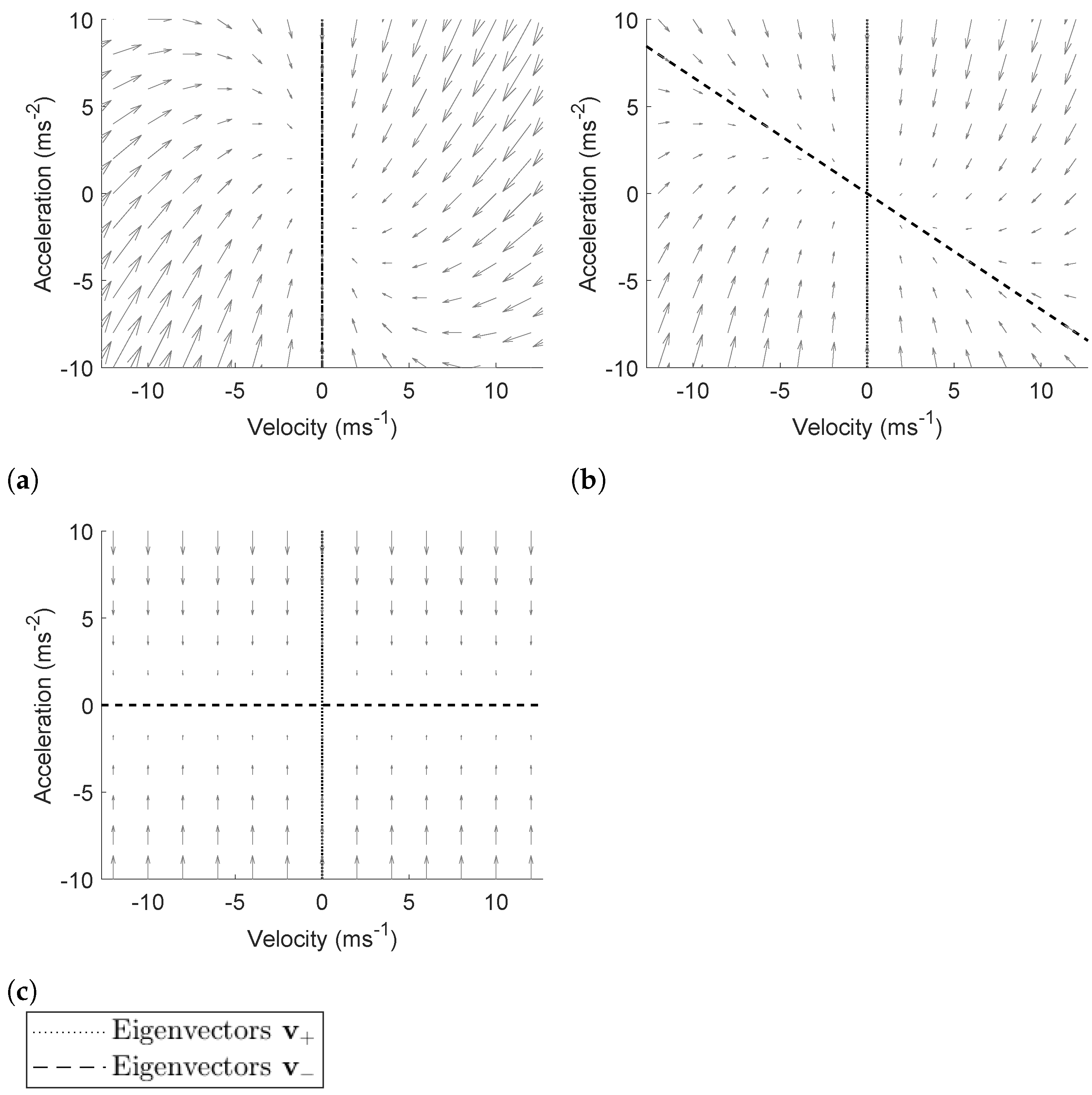
Figure 2a–c are phase-space plots that describe the effect of the linear dependencies of the system (i.e., the deterministic term) for , and . In these plots, each state vector (e.g., , ) describes a single point. The arrows in the phase-space plots show the direction of change from to and the length of the arrows is proportional to the magnitude . The arrows in the phase-space plots show that the linear dependencies described by always cause the state vector to asymptotically converge towards the origin for .
The phase-space plots do not show the exact location of on the plots. It can be shown that always lies on the line
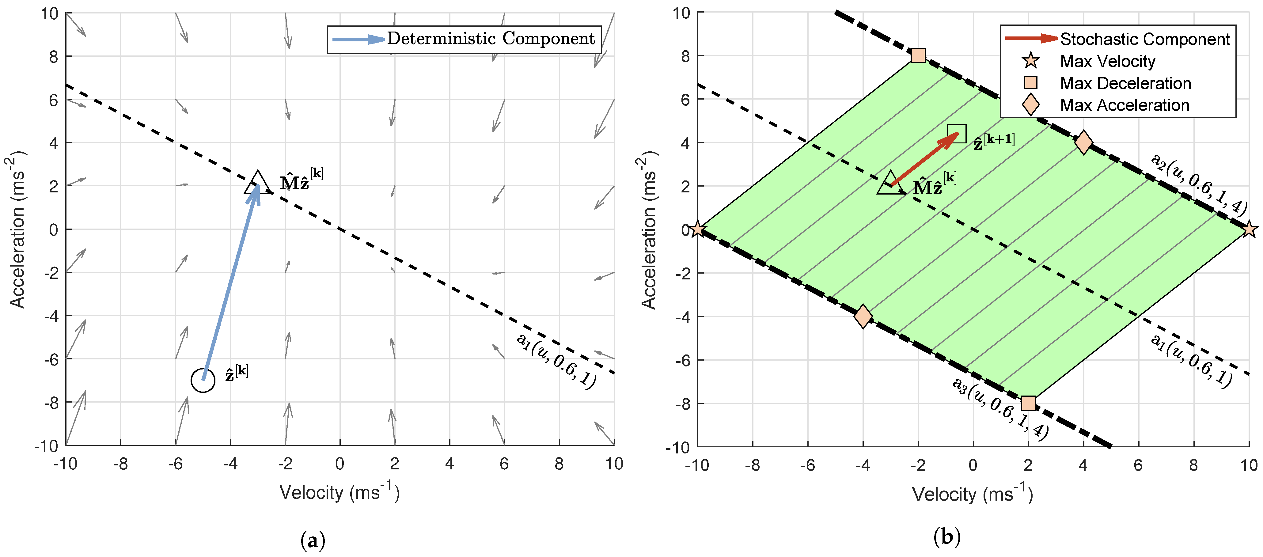
For proof, see Appendix A. Combining this with Figure 2a–c, it is possible to completely predict the location of for any , as shown in Figure 3a.
With the location of known, the possible locations of can now be calculated. It is possible to show that always lies in between the lines
For proof, see Appendix A.1. An example of this can be also seen in Figure 3b.
3.3.3. Derivation of Extreme Cases
Lastly, the purpose of this analysis was to identify the relationship between maximum velocity and acceleration and the values of and . It can be shown that there will always exist an asymptotically maximum velocity given by
such that . For proof see Appendix A.2. Figure 3b (green/shaded region) illustrates all the possible locations of , when . The stars (★) represent the locations with velocity or .
Similarly, it can be shown that there will always exist a maximum acceleration given by
and an asymptotically maximum deceleration given by
For proof see Appendix A.3. The squares (■) in Figure 3b represent the points of maximum deceleration and the diamonds (◆) the points of maximum acceleration .
To find the maximum magnitude U of the velocity vector it is necessary to equate each of its components to , such that
Similarly,
Finally, it is now possible to find expressions for the behavior coefficient and inertia weight in terms of , , U, d and that consider the physical capabilities of the robots
Equation (32) can be difficult to use in its current form. To simplify it, a new parameter is introduced. In (32), it must be the case that and , in order for to be satisfied. That means that the larger the maximum acceleration is compared to the maximum velocity, the smaller must be to ensure stability of the system. Therefore, and can be also expressed using
Following this, it can be made sure that satisfies the conditions of (16) using
3.4. Generalized Adapted PSO
The analysis presented can now be applied to a more general velocity update equation that has an arbitrary number of n acceleration terms. Let us define the velocity update equation of the Generalized Adapted PSO as
where , , …, are locations in the real world and
Please note that the coefficients , … do not have a name at this stage. Equation (35) is algebraically equivalent to (17) if
and
Therefore, it is now possible to apply the analysis presented in this paper, starting from Section 3.3, to the Generalized Adapted PSO algorithm. The rest of this section will outline design guidelines explaining how the Generalized Adapted PSO can be tuned to ensure that it outputs the desired maximum velocity and acceleration. Afterwards, the next section will show how RPSO can be adapted so that it is described by Generalized Adapted RPSO and how the design guidelines can be used to properly implement DVC (see Section 2.2.1) to avoid collisions with obstacles.
3.5. Guidelines
It is now possible to provide a set of design guidelines for the application of the Generalized Adapted PSO to swarm robotic tasks. The parameter selection steps are as follows:
- Identify the controller loop delay: needs to be large enough to accommodate the time delay introduced by computationally expensive tasks and communications between robots.
- Identify U: The desired maximum speed of the robot. It must be made sure that this does not exceed the actual maximum speed that the robot can achieve.
- Calculate either or : The desired maximum acceleration or deceleration using (33). It must be made sure that they do not exceed the actual maximum acceleration or deceleration that the robot can achieve.
- Calculate and : Use (31) and (32) respectively.
- Ensure that and satisfy the criteria of (16): If not, then a faster controller is required (i.e., smaller )
- Select appropriate values for , , …, : The sum of the individual coefficients must satisfy (37).
Traditional guidelines for PSO tuning in parameter optimization tasks aim to control the convergence properties of the swarm (e.g., faster convergence, exploration/exploitation tendencies etc.). This is because in original PSO, the PSO parameters are directly linked to the convergence behavior of the swarm. In Generalized Adapted PSO though, the PSO parameters are primarily used to provide optimal control of the robots. The guidelines provided ensure that the values of , , , …, are properly tuned to provide the desired maximum velocity and acceleration, which will often be the physical maximum velocity and acceleration of the robot. Increasing the values of these parameters further will not result in faster convergence, and it can cause desynchronization between the PSO controller and the robot, resulting in poor control. Therefore, if faster convergence is required, robots with higher maximum velocity and acceleration need to be used. The practitioner can still control the exploration/exploitation tendencies of the swarm, by adjusting the values of , , …, , like in the original PSO, but the limitations and guidelines provided in this paper should also be followed.
Generalized Adapted PSO can become more computationally intensive, the more terms are added to the velocity update equation. Nevertheless, due to the simplicity of the algorithm, it is expected to be computationally simple compared to other tasks that robots usually need to perform (e.g., distance measurement using LiDAR, communication, vision etc.). On the other hand, other computationally intensive tasks may interfere with the operation of Generalized Adapted PSO. To avoid this, the value of needs to be carefully selected. The timestep size is a powerful feature of Generalized Adapted PSO that allows the robot to predict its state in the next timestep. Therefore, as long as accommodates all possible delays, it can ensure optimal control of the swarm.
4. Application to a Real-World System
In contrast to previous work, the analysis presented in this paper focuses on the timestep-to-timestep behavior of the robots. Therefore, (31) and (32) can be used to dynamically adjust the Generalized Adapted PSO parameters independently for each robot, based on the maximum velocity and acceleration that are desired at any time. This can be achieved by using the guidelines of Section 3.5. This is a novel and important capability, and an absolute necessity for the implementation of DVC. To showcase the importance of this capability, and the power of DVC, several simulations were performed.
4.1. Implementation of Dynamic Velocity Control
The following algorithm aims to dynamically adjust the RPSO parameters at each timestep, to control the maximum velocity of each robot. The algorithm forces the robot to move at lower speeds, the closer it is to obstacles or other robots. When implemented correctly, this can prevent collisions with obstacles and other agents.
First, it is important to bound each accelerating term of (9), using the sgn function. Therefore, the RPSO velocity update equation becomes
Now (31) and (32) can be used to dynamically re-calibrate the RPSO parameters at every timestep (given that ). Thus, the robot can slow down in the presence of an obstacle so that it is easier to avoid. In order to perform this dynamic re-calibration (the list of distances to the nearest obstacles) is sorted in order from smallest to largest, such that is the distance to the closest obstacle. Similarly, let
be a vector of speeds, such that is the minimum speed required for the robot to collide with the closest obstacle in the next timestep. The value can be used to prevent collision with obstacle p by selecting a desired maximum speed U using
where . The value of can be reduced to accommodate for a larger error in odometry and distance measurements. From here, the RPSO parameters are calibrated using the guidelines of Section 3.5. The calibration strategy follows three main steps.
Step 1: The sum must be small enough to ensure that at least for the next timestep, it will be impossible for the robot to collide with the closest obstacle. In this case, is assumed to be 0 and . This addresses the case where the robot is not repelled by the closest obstacle at a specific timestep, because happens to be small.
- Set the desired maximum speed .
- Using (33), calculate the desired maximum acceleration .
- Using (31), .
- Using , calculate and based on the desired ratio .
Step 2: The sum must be small enough to ensure that at least for the next timestep, it will be impossible for the robot to collide with the second closest obstacle. This prevents the problematic case where while being repelled by the closest obstacle, the robot ends up colliding with another obstacle. In this case, . As before,
- Set the desired maximum speed .
- Using (33), calculate the desired maximum acceleration . Please note that needs to be the same as in the previous step, in order to result in the same value for as described in (34).
- Using (31), .
- Finally, .
Step 3: The inertia weight can be calculated using (34). One important characteristic of this calibration strategy is that when , then . This means that when the robot is at an equal distance from two obstacles, there is no repulsive effect on the robot, allowing it to pass through the obstacles. This will happen no matter how big the opening is between the obstacles, as long as the robot can fit through it.
5. Results
To demonstrate the performance of the DVC algorithm proposed in Section 4.1, a number of simulations were performed in MATLAB and Gazebo [27]. The MATLAB simulations were idealized, whereas the Gazebo simulations included a more detailed real-time physics model where the inertia of the robots is applied. The algorithms compared in the simulations are:
- The original RPSO algorithm described by (9) with constant parameters.
- The adapted RPSO algorithm described by (38) with constant parameters.
- The adapted RPSO algorithm described by (38) with DVC.
5.1. World and Robot Description
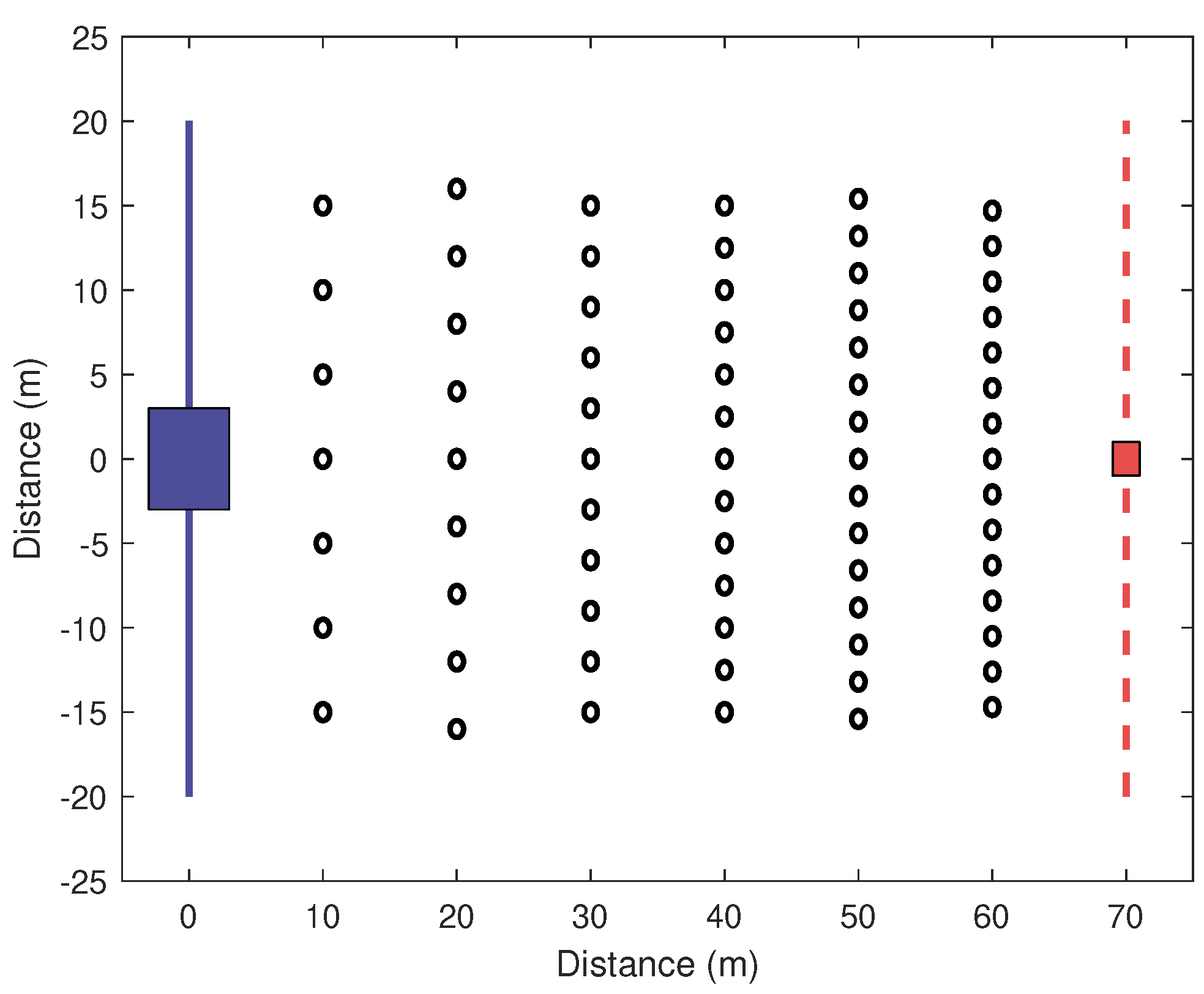
The world used in all simulations is shown in Figure 4, the blue square is the area where the robots are initialized, the red square is the target (global minimum of the cost function, the cost is equal to the distance between the robot and the source) and the circles are obstacles. The obstacles become denser the closer to the target.
Swarm intelligence algorithms such as PSO are inherently scalable [13]. That means that the same algorithm should be applicable to large swarms (>100 robots) and small swarms (<20 robots) without additional tuning. That said, there is a minimum number of robots required for a swarm to be effective. In this paper, it was chosen to demonstrate the new PSO algorithms on a small swarm of 6 robots. The robots of the swarm are based on the Robotnik Summit XL Steel platform [28], a popular robotic platform with available specifications and simulation models (e.g., Gazebo models). The robots can move within the two-dimensional world, and collisions with obstacles or other robots can occur. If a collision occurs the robot is considered to become disabled and cannot move any further. The robots are assumed to have unlimited communication range and bandwidth, and each robot can communicate with every other robot in the swarm at all times.
A low-cost obstacle-detection short-range LiDAR sensor can have maximum range starting from 4 [29], so the obstacle-detection range was set to 3 , to avoid operating at the sensor’s maximum range. Due to the way that the Gazebo simulations operate, a robot can detect obstacles in its detection range even if they are “hidden” behind other obstacles. This contradicts how a LiDAR would detect obstacles and it can result in multiple repulsive forces being exerted from the same direction. To avoid this, each robot separates its surroundings into six equally sized radially separated regions. Only the repulsive forces exerted by the closest body in each region are accounted for the calculation of the total repulsive force.
The robots are limited to 3 / maximum speed (the actual maximum speed of the Summit XL Steel). The actual maximum acceleration of Summit XL Steel is not available, but it is assumed to be very high, since it uses electric motors which are characterized by high acceleration. To achieve a large , the weight must be also large and therefore needs to be small (see (33) and (34)).
The cognitive coefficient allows the robot to explore the environment around it and overcome obstacles, while the social coefficient encourages the robot to move towards the global best location . As both coefficients are of importance in source localization tasks it is assumed that
The values for , and can be either constant or dynamic at every timestep. Both scenarios will be studied in the following simulations.
5.1.1. Original RPSO with Constant Values
For the original RPSO algorithm, the magnitudes of the single values , and rarely matter. This is because it is very easy for the resulting velocity of the algorithm to be higher than the maximum velocity of the robot. Instead, what matters is the ratio , as it is also suggested by the original RPSO work, since this will control the direction of the requested velocity. In order to allow direct comparison between the algorithms, the same cases will be used for the original RPSO, as for the adapted RPSO with constant values.
5.1.2. Adapted RPSO with Constant Values
In the case of the adapted RPSO, all the terms of the velocity update equation are bounded using the sgn function. Therefore, it is possible to tune the parameters using (31) and (32). The parameters are tuned so that the desired maximum velocity U is always equal to the physical maximum velocity of the robot. The desired maximum acceleration can be calculated using (33). From here, it is now possible to calculate the values of , and , based on the desired value of the ratio . For the following simulations, three cases will be tested: , , and .
5.1.3. Adapted RPSO with DVC
For adapted RPSO with DVC, , and will be recalibrated at every timestep for each robot depending on its current state, as explained in Section 4.1. Lastly, the simulations were created to resemble typical real-world robotic applications (e.g., a swarm of drones navigating through a forest or a city). The values of some of the parameters used (, , , and ) were selected heuristically to match such applications. Changing the value of the parameters , , and is expected to affect all cases in the same way. In the case of , it is only used by one of the tested cases (adapted PSO with DVC) and optimization of this parameter is beyond the scope of this paper. Table 1 shows the values assigned to these parameters throughout all the simulations, along with the values of the parameters , and for each tested case.
To assess the performance of each swarm, the fitness of the swarm is calculated using
where the right-hand side of the equation is the horizontal distance from the origin to the Center of Mass (CoM) of the swarm. As previously mentioned, robots that have collided with obstacles or other robots are considered to be “collided”. The percentage of robots that have collided by the end of the simulation is also used as a secondary metric.
5.2. MATLAB Simulations
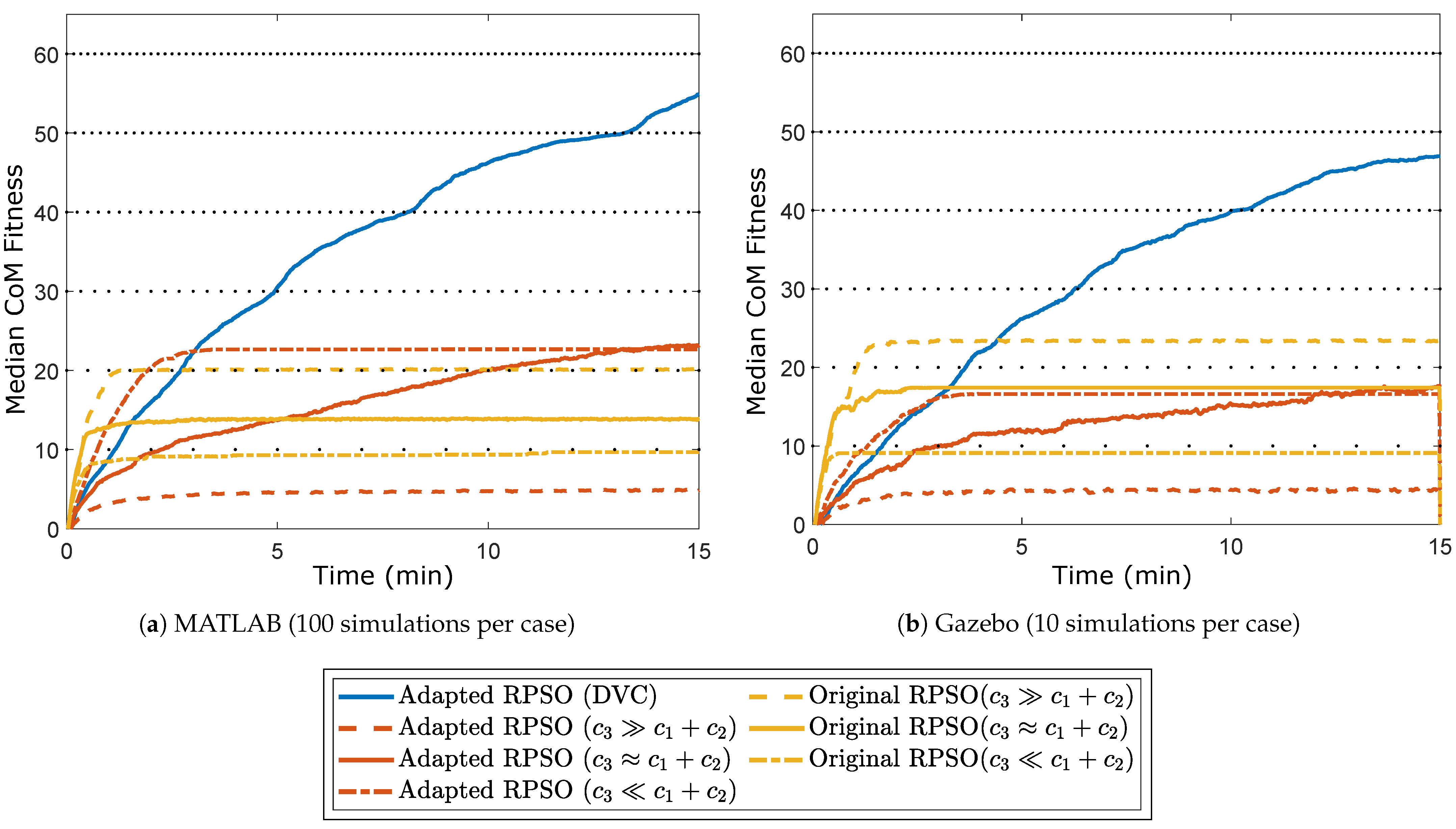
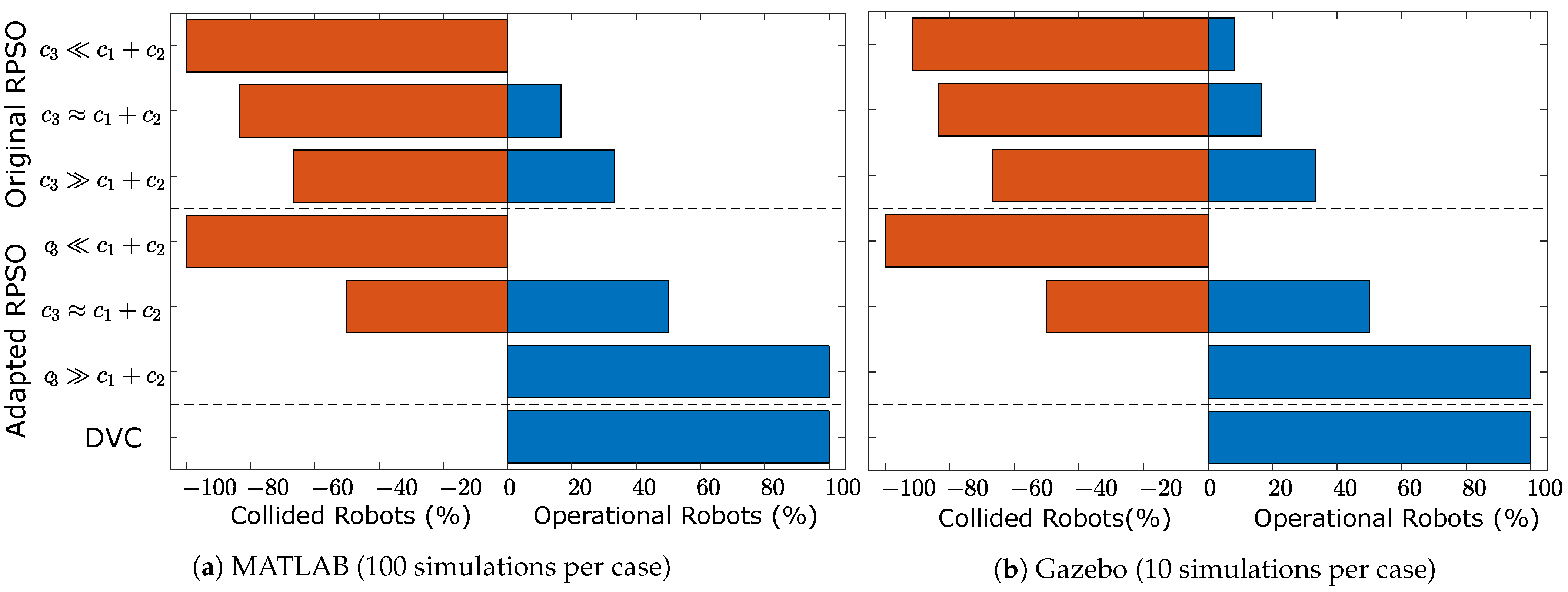
MATLAB was used to simulate the swarm over 100 repeats, with no physics engine. This number of simulations was selected because it could produce a clear behavioral trend for each algorithm. Figure 5a shows the median CoM fitness over time for each algorithm and Figure 6a shows the median number of collided vs operational robots at the end of the simulation.
As it can be seen from the results of Figure 5a, with adapted RPSO with DVC, the CoM of the average swarm manages to pass through the fifth layer of obstacles (fifth dotted line) before the end of the simulation. This contrasts with the other algorithms that do not manage to pass through the third layer. All cases of the original RPSO appear to progress quickly at the beginning, this is in fitting with the fact that the original RPSO almost always operates at the maximum velocity permitted by the physical constraints of the robot. On the other hand, all cases of the adapted RPSO (including DVC) progress more slowly.
In Figure 6a, it can be seen that all cases of both the original RPSO and the adapted RPSO follow the predicted behavior, i.e., as gets larger compared to , the number of collisions decreases. For small , adapted RPSO results in only collisions, while for large , it results in no collisions. All the cases of original RPSO however have very low survivability.
Lastly, the only cases that end up with absolutely no collisions are the adapted RPSO with large and the adapted RPSO with DVC. Comparing the two cases in Figure 5a, it can be seen that the adapted RPSO with large has the lowest overall fitness out of all cases. In contrast, the adapted RPSO with DVC has the highest overall fitness. This shows that the adapted RPSO with DVC completely overshadows all other cases, both in terms of fitness and robot survivability. This is attributed to the DVC strategy used. The strategy makes use of the velocity boundaries introduced by adapted RPSO, to slow down a robot in the presence of an obstacle, making it practically impossible to collide with any obstacles or other agents. At the same time, the robot is still capable of navigating through small openings; a capability that is not shared by the other two algorithms.
5.3. Gazebo Simulations
To expand on the results of the MATLAB simulations, a number of more realistic simulations were run in Gazebo (benefiting from a detailed Physics Engine). The robots are equipped with contact sensors to detect collisions and with mecanum wheels for holonomic motion. The motion of the robots is governed by the forward and inverse kinematic equations of the mecanum wheels [30]. The robots move by forces being applied on them and they have inertia. Please note that for the Gazebo simulations, apart from the high-level swarm behavior controller described by each studied RPSO case, each robot also employs underlying low-level motor controllers and data collection nodes that operate at a higher refresh rate. The timestep used for these controllers is .
Figure 5b and Figure 6b show the median CoM fitness over time and the median number of collided vs operational robots for each tested case, respectively. Comparing Figure 5a,b, it can be seen that there are small differences. Specifically, there is a small reduction in the overall performance of the adapted RPSO cases, which can be probably attributed to the imperfect motion of mecanum wheels (i.e., the maximum speed of the robot is limited when it is moving towards certain directions). However, the adapted RPSO with DVC performs better than the other algorithms, reaching an average fitness of 47 by the end of the simulation. When it comes to Figure 6a,b, the results look almost identical for all cases. The original RPSO with appears to have limited survivability that is not observed in the MATLAB simulations.
6. Discussion
This paper has introduced a modified version of the Particle Swarm Optimization algorithm, called Adapted PSO, for use as a robot controller in robotic swarms. This was achieved by bounding the terms of the PSO velocity update equation using the sgn function and by including the timestep size . A PSO parameter selection process was also formalized, by analysing the timestep-to-timestep behavior of a PSO particle. The new parameter tuning equations offer direct control of the desired maximum velocity and maximum acceleration of each robot.
To validate the proposed changes, another modified PSO algorithm called Robotic-PSO (RPSO) that includes obstacle avoidance, was adapted according to the proposed guidelines. The parameter tuning equations were also used to dynamically retune the parameters of Adapted RPSO in real time; a process called Dynamic Velocity Control (DVC). Adapted RPSO was compared to original RPSO in simulations, and it was shown to offer significantly better control over the swarm. Adapted RPSO with DVC was able to navigate inside a difficult environment of obstacles without resulting in any collisions. This contrasts with the original RPSO which was not able to navigate far into the environment and almost always resulted in collisions.
The inclusion of the sgn function effectively bounds the terms of the velocity update equation, addressing Problem 1. The inclusion of the parameter in the parameter tuning equations solves the synchronisation problem between the PSO position and velocity update equations, addressing Problem 2. The effect of this can be directly seen in the results of Section 5.2 and Section 5.3, where 1 . Such a large loop delay is typically unsuitable for most applications of this scale (1–100 ) as it can result in collisions and poor control of the robot. That being said, adapted RPSO with DVC controls the swarm such that robots of diameter 1 can pass through openings of size without any risk of colliding, even when such a large value of is used.
In its current form, the PSO controller presented in this paper can be used for tasks that require the swarm to move to a certain location by setting the global best location as that location. It is furthermore possible to use the algorithm in several source localization and tracking tasks (i.e., source localization using olfaction). That being said, for PSO to be used as a generalized source localization algorithm, Problems 3 and 4 still need to be overcome. Nevertheless, there already exist candidate solutions. For example it might be possible to overcome the limitation that PSO needs to operate in an immutable environment (Problem 3), by slowly increasing the cost of the current personal best and global best locations exponentially, forcing the robot to re-update them. The performance of these candidate solutions can now be properly implemented on simulated and physical swarms using the methods proposed in this paper, ensuring that the operation of the swarms will not be affected by Problems 1 and 2.
Finally, the adaptation of RPSO in this paper provides a direct application of the adapted PSO algorithm presented. The performance of Adapted RPSO with DVC in Section 5.2 and Section 5.3 shows that it is possible to incorporate different tasks into the Generalized Adapted PSO velocity update equation as individual terms and control them by re-calibrating the PSO parameters at each timestep. Similarly, it might be possible to incorporate other tasks (e.g., flocking, target trapping and pattern formation) into the Generalized Adapted PSO equation as additional PSO terms. Each task is run separately from the rest and they are all merged by the Generalized Adapted PSO velocity update equation. The practitioner needs only to identify a simple strategy for the re-calibration of the PSO parameters that will control which tasks are given more importance in different situations. In this way, the Generalized Adapted PSO velocity update equation takes the form of a general swarm control framework for robotic swarms. Such a framework could eventually lead to the standardization of swarm intelligence algorithms.
The work presented is generalized, and there exist many parameters that can affect the behavior of the robot that could be further included into the tuning process. Some of the most important are minimum turning radius, maximum rotational speed and maximum rotational acceleration. These characteristics represent significant obstacles in the use of PSO as a controller for the traditional non-holonomic robots (e.g., differential drive, traditional steering, forward flight etc.).
7. Conclusions
This paper introduced a new PSO algorithm called Adapted PSO and formalized parameter selection guidelines that specifically enable the application of PSO as a controller in robotic swarms. This has been achieved by considering the physical properties of the robots, including the desired maximum velocity and acceleration, and relating these to the inertia weight and the cognitive and social coefficients via a state model. Coupled with the introduction of the controller loop delay, these new guidelines also guarantee both order-1 and order-2 stability. Thus, solving the two key problems (lack of constraints and asynchronous control) that have so far limited the formal application of PSO to the control of robotic swarms. The new algorithm is compared to original PSO in simulations, and it is shown to excel both in terms of navigation through a difficult environment and robot survivability.
Author Contributions
Conceptualization, G.R., B.M., A.H.; methodology, G.R., B.M., A.H.; software, G.R.; validation, G.R., B.M., A.H.; formal analysis, G.R., B.M., A.H.; investigation, G.R., B.M., A.H.; resources, B.M.; data curation, G.R.; writing—original draft preparation, G.R.; writing—review and editing, G.R., B.M., A.H.; visualization, G.R., B.M., A.H.; supervision, B.M., A.H.; project administration, B.M.; funding acquisition, B.M. All authors have read and agreed to the published version of the manuscript.
Funding
This research and the APC were funded by both the UK Natural Environment Research Council (NERC) and Engineering and Physical Sciences Research Council (EPSRC) grant number NE/N012070/1.
Institutional Review Board Statement
Not applicable.
Informed Consent Statement
Not applicable.
Data Availability Statement
Not applicable.
Conflicts of Interest
The authors declare no conflict of interest. The funders had no role in the design of the study; in the collection, analyses, or interpretation of data; in the writing of the manuscript, or in the decision to publish the results.
Appendix A. Lemma 1
Lemma 1.
For all , will always lie on the line given by:
Proof.
The matrix has eigenvectors
and respective eigenvalues
Matrix is diagonalizable, since it is of size and has 2 distinct eigenvalues. Therefore, the column space of is fully described by the span of the eigenvectors that are associated with non-zero eigenvalues as shown below
This implies that C() is a line and its characteristic equation is given by
and the vector will always lie on it. □
Appendix A.1. Lemma 2
Lemma 2.
For all , the vector will always be located in between the lines
Proof.
The vector is a vector of random magnitude and is always parallel to the line
It has maximum length when
Lemma 1 says that always lies on the line of (23). When as shown in (A4), the vector must lie on the line
Conversely, when , the vector must lie on the line
Therefore, in all other cases, the vector must always be located between the lines and . □
Appendix A.2. Theorem 1
Theorem 1.
For all ω, and , there will always exist a maximum velocity such that
Proof.
To find the value of , let a robot accelerate in a single direction so that
In this case, (A5) represents a non-homogeneous first-order linear recurrence relation. Assuming that and , the maximum velocity is given by
Therefore, if a robot is allowed to accelerate as much as possible towards a specific direction, its velocity will asymptotically approach resulting in for any value of . □
Appendix A.3. Theorem 2
Theorem 2.
For all ω, and , there will always exist a maximum acceleration and a maximum deceleration .
Proof.
The maximum acceleration can be found by setting in (21) and assuming that the sgn function is positive, resulting in
Conversely, the maximum deceleration can be found by setting in (21) and assuming that the sgn function is negative, resulting in
Substituting (A6) in (A8) results in the relationship between and
Equations (26) and (A9) are well-defined expressions of and in terms of , and , under the only conditions that and . Therefore, under these conditions, and . □
References
- Kennedy, J.; Eberhart, R. Particle swarm optimization. In Proceedings of the ICNN’95-International Conference on Neural Networks, Perth, WA, Australia, 27 November–1 December 1995; Volume 4, pp. 1942–1948. [Google Scholar] [CrossRef]
- Parsopoulos, K.E.; Vrahatis, M.N. Particle Swarm Optimization and Intelligence: Advances and Applications; Information Science Publishing (IGI Global): London, UK, 2010. [Google Scholar]
- Liu, C.; Chu, Y.; Wang, L.; Zhang, Y. Application and the parameter tuning of ADRC based on BFO-PSO algorithm. In Proceedings of the 2013 25th Chinese Control and Decision Conference (CCDC), Guiyang, China, 25–27 May 2013; pp. 3099–3102. [Google Scholar] [CrossRef]
- Crawford, B.; Soto, R.; Monfroy, E.; Palma, W.; Castro, C.; Paredes, F. Parameter tuning of a choice-function based hyperheuristic using Particle Swarm Optimization. Expert Syst. Appl. 2013, 40, 1690–1695. [Google Scholar] [CrossRef]
- Pluhacek, M.; Senkerik, R.; Viktorin, A.; Kadavy, T.; Zelinka, I. A Review of Real-World Applications of Particle Swarm Optimization Algorithm BT-AETA 2017-Recent Advances in Electrical Engineering and Related Sciences: Theory and Application; Springer International Publishing: Cham, Switzerland, 2018; pp. 115–122. [Google Scholar]
- Ozcan, E.; Mohan, C.K. Particle swarm optimization: Surfing the waves. In Proceedings of the 1999 Congress on Evolutionary Computation-CEC99 (Cat. No. 99TH8406), Washington, DC, USA, 6–9 July 1999; Volume 3, pp. 1939–1944. [Google Scholar] [CrossRef]
- Trelea, I.C. The particle swarm optimization algorithm: Convergence analysis and parameter selection. Inf. Process. Lett. 2003, 85, 317–325. [Google Scholar] [CrossRef]
- Liu, Q. Order-2 Stability Analysis of Particle Swarm Optimization. Evol. Comput. 2014, 23. [Google Scholar] [CrossRef] [PubMed]
- Bonyadi, M.R.; Michalewicz, Z. Stability Analysis of the Particle Swarm Optimization Without Stagnation Assumption. IEEE Trans. Evol. Comput. 2016, 20, 814–819. [Google Scholar] [CrossRef]
- Cleghorn, C.W.; Engelbrecht, A.P. Particle swarm stability: A theoretical extension using the non-stagnate distribution assumption. Swarm Intell. 2018, 12, 1–22. [Google Scholar] [CrossRef] [Green Version]
- Tan, Y.; Zheng, Z.Y. Research Advance in Swarm Robotics. Def. Technol. 2013, 9, 18–39. [Google Scholar] [CrossRef] [Green Version]
- Nedjah, N.; Junior, L.S. Review of methodologies and tasks in swarm robotics towards standardization. Swarm Evol. Comput. 2019, 50, 100565. [Google Scholar] [CrossRef]
- Senanayake, M.; Senthooran, I.; Barca, J.C.; Chung, H.; Kamruzzaman, J.; Murshed, M. Search and tracking algorithms for swarms of robots: A survey. Robot. Auton. Syst. 2016, 75, 422–434. [Google Scholar] [CrossRef]
- Couceiro, M.S.; Rocha, R.P.; Ferreira, N.M.F. A novel multi-robot exploration approach based on Particle Swarm Optimization algorithms. In Proceedings of the 2011 IEEE International Symposium on Safety, Security, and Rescue Robotics, Kyoto, Japan, 31 October–5 November 2011; pp. 327–332. [Google Scholar] [CrossRef]
- Wang, Z.; Qin, L.; Yang, W. A self–organising cooperative hunting by robotic swarm based on particle swarm optimisation localisation. Int. J. Bio-Inspired Comput. 2015, 7, 68–73. [Google Scholar] [CrossRef]
- Kumar, A.S.; Manikutty, G.; Bhavani, R.R.; Couceiro, M.S. Search and rescue operations using robotic darwinian particle swarm optimization. In Proceedings of the 2017 International Conference on Advances in Computing, Communications and Informatics (ICACCI), Udupi, India, 13–16 September 2017; pp. 1839–1843. [Google Scholar] [CrossRef]
- Hereford, J.M.; Siebold, M.; Nichols, S. Using the Particle Swarm Optimization Algorithm for Robotic Search Applications. In Proceedings of the 2007 IEEE Swarm Intelligence Symposium, Honolulu, HI, USA, 1–5 April 2007; pp. 53–59. [Google Scholar] [CrossRef]
- Clerc, M.; Kennedy, J. The particle swarm-explosion, stability, and convergence in a multidimensional complex space. IEEE Trans. Evol. Comput. 2002, 6, 58–73. [Google Scholar] [CrossRef] [Green Version]
- Kennedy, J. Particle swarm optimization. In Encyclopedia of Machine Learning; Springer: Boston, MA, USA, 2010; pp. 760–766. [Google Scholar]
- Shi, Y.; Eberhart, R.C. Parameter selection in particle swarm optimization. In Evolutionary Programming VII; Springer: Berlin/Heidelberg, Germany, 1998; pp. 591–600. [Google Scholar]
- Poli, R. Dynamics and Stability of the Sampling Distribution of Particle Swarm Optimisers via Moment Analysis. J. Artif. Evol. Appl. 2008, 2008. [Google Scholar] [CrossRef] [Green Version]
- Spears, W.M.; Spears, D.F.; Hamann, J.C.; Heil, R. Distributed, Physics-Based Control of Swarms of Vehicles. Auton. Robot. 2004, 17, 137–162. [Google Scholar] [CrossRef]
- Khaldi, B.; Cherif, F. A Virtual Viscoelastic Based Aggregation Model for Self-Organization of Swarm Robots System; Lecture Notes in Computer Science (Including Subseries Lecture Notes in Artificial Intelligence and Lecture Notes in Bioinformatics); Springer: Cham, Switzerland, 2016; Volume 9716, pp. 202–213. [Google Scholar] [CrossRef]
- Garone, E.; Nicotra, M.; Ntogramatzidis, L. Explicit reference governor for linear systems. Int. J. Control 2018, 91, 1415–1430. [Google Scholar] [CrossRef]
- Hosseinzadeh, M.; Garone, E. An Explicit Reference Governor for the Intersection of Concave Constraints. IEEE Trans. Autom. Control 2020, 65, 1–11. [Google Scholar] [CrossRef]
- Utkin, V. Chattering Problem. IFAC Proc. Vol. 2011, 44, 13374–13379. [Google Scholar] [CrossRef]
- Koenig, N.; Howard, A. Design and use paradigms for Gazebo, an open-source multi-robot simulator. In Proceedings of the 2004 IEEE/RSJ International Conference on Intelligent Robots and Systems (IROS) (IEEE Cat. No.04CH37566), Sendai, Japan, 28 September–2 October 2004; Volume 3, pp. 2149–2154. [Google Scholar] [CrossRef] [Green Version]
- Robotnik Automation S.L.L. SUMMIT-XL STEEL MOBILE ROBOT. Available online: https://robotnik.eu/products/mobile-robots/summit-xl-steel-en (accessed on 10 January 2021).
- Benewake (Beijing) Co., Ltd. CE30 3D Obstacle-Avoidance LiDAR. Available online: http://en.benewake.com/product/detail/5c34571eadd0b639f4340ce5 (accessed on 15 February 2021).
- Taheri, H.; Qiao, B.; Ghaeminezhad, N. Kinematic model of a four mecanum wheeled mobile robot. Int. J. Comput. Appl. 2015, 113, 6–9. [Google Scholar] [CrossRef]
Figure 1.
The safe operating regions defined by allowable values of that guarantee order-1 and order-2 stability.
Figure 1.
The safe operating regions defined by allowable values of that guarantee order-1 and order-2 stability.

Figure 2.
The phase-space graph for three different cases: (a) , (b) (in this specific case ), (c) . In all three cases the system is stable. Also, in (a) (extreme case) and (b) (normal case), the system is asymptotically convergent towards the origin.
Figure 2.
The phase-space graph for three different cases: (a) , (b) (in this specific case ), (c) . In all three cases the system is stable. Also, in (a) (extreme case) and (b) (normal case), the system is asymptotically convergent towards the origin.

Figure 3.
Example that shows the deterministic effect of (a) and the stochastic effect of (b) on a random position of , for , and . No matter the location of , the point will always be located closer to the origin, lying on . The point will always be located in between the lines and . The vector is always parallel to the hatching lines of the shaded-hatched region, which have gradient . The shaded-hatched region represents all possible states . For this system, , and .

Figure 4.
The obstacle map used in both MATLAB and Gazebo simulations. The blue square on the left shows the starting area where robots are initialized and the red square on the right shows the position of the target. The obstacles become denser the closer to the target.
Figure 4.
The obstacle map used in both MATLAB and Gazebo simulations. The blue square on the left shows the starting area where robots are initialized and the red square on the right shows the position of the target. The obstacles become denser the closer to the target.

Figure 5.
Median CoM fitness over time results for different cases. The dotted lines represent the obstacle layers of the obstacle course.
Figure 5.
Median CoM fitness over time results for different cases. The dotted lines represent the obstacle layers of the obstacle course.

Figure 6.
The expected number of collided vs operational robots at the end of the median simulation for different cases.
Figure 6.
The expected number of collided vs operational robots at the end of the median simulation for different cases.


Table 1.
Table of values used for different parameters.
| Algorithm | Case | ||||||
|---|---|---|---|---|---|---|---|
| Adapted RPSO | DVC | 0.9 | 0.9 | 1 | 1 | - | - |
| - | 0.9 | 1 | 1 | 0.2864 | 1.1455 | ||
| 0.4296 | 0.8591 | ||||||
| 0.5728 | 0.5728 | ||||||
| Original RPSO | - | 0.9 | 1 | 1 | 0.2864 | 1.1455 | |
| 0.4296 | 0.8591 | ||||||
| 0.5728 | 0.5728 |
Publisher’s Note: MDPI stays neutral with regard to jurisdictional claims in published maps and institutional affiliations. |
© 2021 by the authors. Licensee MDPI, Basel, Switzerland. This article is an open access article distributed under the terms and conditions of the Creative Commons Attribution (CC BY) license (https://creativecommons.org/licenses/by/4.0/).
Share and Cite
MDPI and ACS Style
Rossides, G.; Metcalfe, B.; Hunter, A. Particle Swarm Optimization—An Adaptation for the Control of Robotic Swarms. Robotics 2021, 10, 58. https://0-doi-org.brum.beds.ac.uk/10.3390/robotics10020058
AMA Style
Rossides G, Metcalfe B, Hunter A. Particle Swarm Optimization—An Adaptation for the Control of Robotic Swarms. Robotics. 2021; 10(2):58. https://0-doi-org.brum.beds.ac.uk/10.3390/robotics10020058
Chicago/Turabian StyleRossides, George, Benjamin Metcalfe, and Alan Hunter. 2021. "Particle Swarm Optimization—An Adaptation for the Control of Robotic Swarms" Robotics 10, no. 2: 58. https://0-doi-org.brum.beds.ac.uk/10.3390/robotics10020058
Note that from the first issue of 2016, this journal uses article numbers instead of page numbers. See further details here.