
Trajectory Extrapolation for Manual Robot Remote Welding


1
Institute for Material Science and Welding Techniques, University of Applied Science Hamburg, Berliner Tor 5, 20099 Hamburg, Germany
2
Research and Transfer Center FTZ-3i, University of Applied Science Hamburg, Berliner Tor 5, 20099 Hamburg, Germany
*
Author to whom correspondence should be addressed.
†
These authors contributed equally to this work.
Robotics 2021, 10(2), 77; https://0-doi-org.brum.beds.ac.uk/10.3390/robotics10020077
Submission received: 15 April 2021
/
Revised: 16 May 2021
/
Accepted: 20 May 2021
/
Published: 23 May 2021
(This article belongs to the Topic Motion Planning and Control for Robotics)
Abstract
:This article describes an algorithm for the online extrapolation of hand-motion during remote welding. The aim is to overcome the spatial limitations of the human welder’s arms in order to cover a larger workspace with a continuous weld seam and to substantially relieve the welder from strain and fatigue. Depending on the sampled hand-motion data, an extrapolation of the given motion patterns is achieved by decomposing the input signals in a linear direction and a periodic motion component. An approach to efficiently determine the periodicity using a sampled autocorrelation function and the subsequent application of parameter identification using a spline function are presented in this paper. The proposed approach is able to resemble all practically relevant motion patterns and has been validated successfully on a remote welding system with limited input space and audio-visual feedback by an experienced welder.
1. Introduction
To decrease programming effort, improve ergonomics, and reduce hazards to the welder, remote welding applications are pursued [1,2,3,4,5,6,7,8,9]. The typical setup consists of a motion input device and a standard industrial robot with a welding torch attached. The input devices range from complex applications of VR technology [10] to simpler methodologies using infrared optical motion sensors [11,12]. A comprehensive overview of different approaches is given in Section 3 of the review paper [13]. The common problem with those approaches is the limited tracking region of the input device, whereas longer, and even more important, continuous welding seams are to be manufactured [14]. To achieve these long continuous welding seams, solutions have been presented [15,16,17,18] that apply 2D laser-scanning before the welding in order to pre-calculate a trajectory. However, it is still beneficial to directly control the torch’s motion to save time and to respond to unexpected variations in material properties, as they are frequently present in repair applications [19].
Recent work performed by the authors of the paper [20] introduces a promising approach to tackle the problem of the limited workspace of the motion input devices, as illustrated in Figure 1. When the motion of the input device, which is tracked by the robot, reaches the boundary of the input device’s acquisition space, the robot’s motion is continued by extrapolation of the input trajectory for a period of time. In the meantime, the input device can be re-positioned into a convenient position and the control is resumed to the tracking of the input device thereafter. The extrapolation algorithm uses a discrete Fourier transformation (DFT) approach to isolate the dominant spatial frequency and is able to generate the continuous motion pattern for the weaving motion in concave and convex shapes by estimating parameters of a sine template function. As a result, spatial motions must be composable by a single sine function per degree of freedom. Thus, the practically relevant Christmas-tree-shaped motion pattern is extrapolated with limited fidelity only and the algorithms proposed in the paper [20] still have to be validated in practical welding experiments.
In this paper, we introduce an approach based on a sampled autocorrelation function and a spline parameter estimation that is applicable to the practically relevant straight line, weaving, and Christmas-tree-shaped (see the publication [21]) motion patterns. Successful experimental results using real-life input motion data and practically performed remote welding validations are presented and discussed.
2. Problem Description
For the input device, the coordinate system depicted in Figure 2 is applied. A dummy torch tracked by a stereoscopic vision system is used and the main motion is performed in the y-z-plane. Details of the signal processing and the integration into the robot control are given in Section 4.1 of this article.
A Christmas-tree-shaped input trajectory obtained from a practical weld is depicted in Figure 3.
This is the trajectory to be extrapolated in order to achieve a continuous weld and the control by the input device has to be resumed afterward without causing any discontinuities in torch position and velocity. The proposed algorithm has been successfully applied to straight-line and weaving motion patterns, but the discussion in the following section is based on the most complex motion pattern shape, the Christmas tree shape. It can be seen from the data that compared to synthetic signals a lot of hand tremor is present, which is quite typical for manual welding [22,23,24].
The following goals must be met:
- The overall direction of the welding seam must be kept. Therefore, the linear motion components must be isolated from periodic ones.
- The macroscopic shape of the weld must be kept so that the outer geometry of the seam still connects the workpieces properly.
- Tremor-induced microscopic motion must not be mistaken for a periodic macroscopic motion pattern.
3. Extrapolation Algorithm
The extrapolated robot trajectory is calculated for the motion in the y-z-plane, whereas the last measured angles , , and , as well as the last measured x-coordinate, are kept constant during extrapolation. Equations are given for the y-coordinate of the plane only; the motion in the z-direction is calculated analogously.
The first step of the algorithm determines the overall direction of the weld and distinguishes between linear motion with tremor present and an intended periodic welding motion pattern.
3.1. Motion Linear Direction and Periodic Component Frequency Estimation
The input signal captured by the vision system at the sample times is split in its Cartesian components and modeled according to Equation (1) for each component in order to estimate the linear motion parameters (axis intercept) and (slope).
In Equation (1), is the vector containing the y-component of the input signal over time. denotes a vector representing the residuals of the parameter estimation problem, which are unknown as well as the parameters . The affine linear parameters are determined by QR-decomposition of the regressor matrix using the Armadillo math package [26,27] over 15 s of measurement data and denoted as . After this parameter estimation, the residual signal vector is calculated by
which removes the linear components from the signal and the RMS value of the residual signal is used to determine if tremor motion only or a significant intended periodic motion are present in the signal. A threshold value is chosen empirically from the measured motion patterns as shown in Figure 3. The periodic welding pattern shows a motion amplitude that is significantly larger than the tremor component, which is typically lower than a threshold of 3 mm. This value is determined by letting welders draw a straight line by hand at a typical welding speed of 10 mm/s and measuring the RMS value of the tremor.
If the threshold is not exceeded, the extrapolation is performed by
where and are the elements of the estimated vector , k is the index of the extrapolation signal and T is the sample time period.
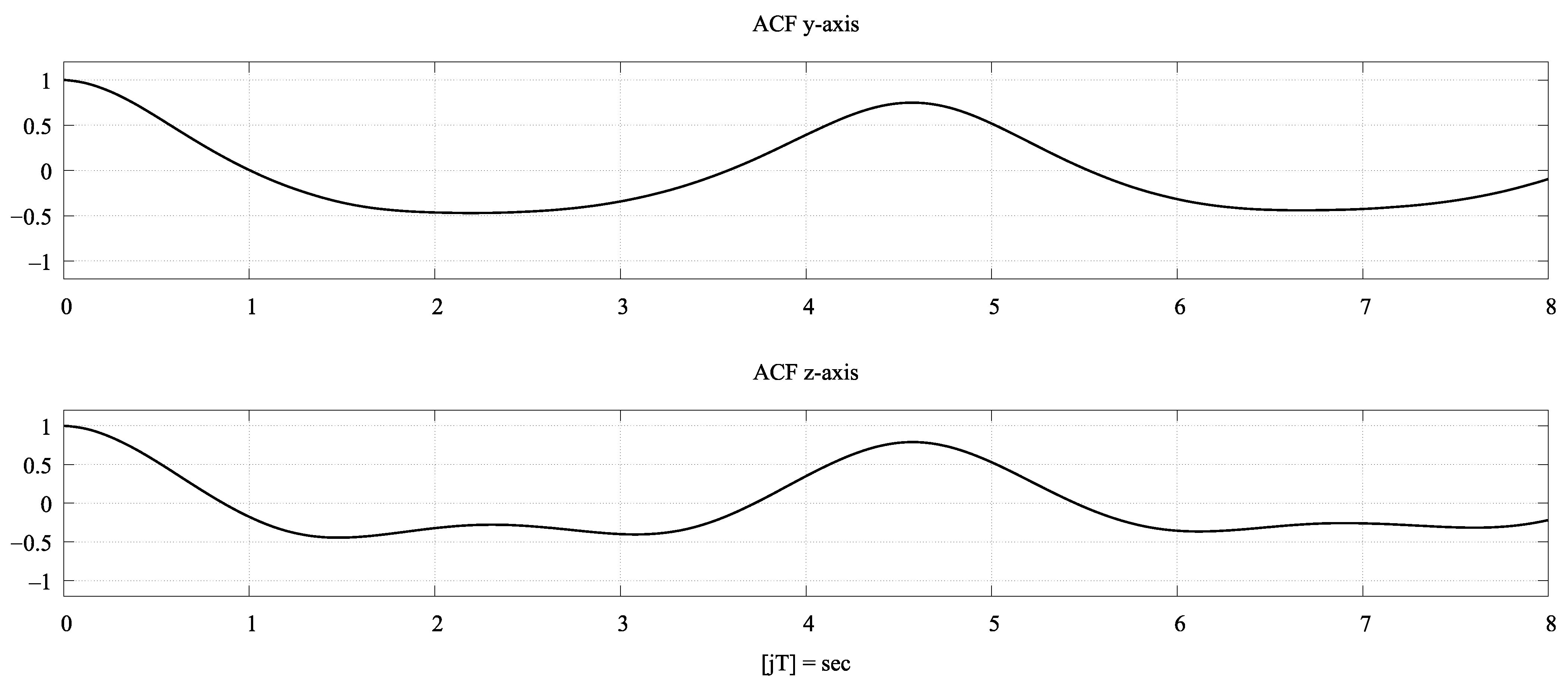
If the threshold for the tremor-only motion is exceeded and thus, a significant periodic motion pattern is present in the residual vector , the period of the most prominent frequency is estimated by calculating the autocorrelation function of the signal according to Equation (4).
Figure 4 shows the plot of the autocorrelation function (ACF) calculated from the measured welding motion depicted in Figure 3. The highest maximum is always found at zero time delay, resulting from a perfect correlation of the signal with itself. The second-highest maximum represents the most significant periodic motion frequency determined by its time delay .
To identify the second-highest maximum efficiently, Equation (4) is calculated at a discrete number of equally spaced probe points first and then evaluated for a possible region in which to find it. Candidate regions are determined by all probe points that have two lower neighbor probe points. Then, from these points, the candidate with the highest value is chosen. As a result, the left index l and the right index r of the neighbors are used and the dominant motion frequency is therefore determined by a linear search according to Equation (5).
This approach reduces the computational effort of the dominant motion frequency identification, since the computationally expensive autocorrelation function has to be calculated for the probe points and the samples contained in the interval , only.
3.2. Periodic Motion Generation
In the case that the input motion is not determined as a straight line, a periodic motion pattern has to be continued by the extrapolation algorithm as a second step. After estimating the frequency of the periodic motion, the last signal period is used to fit spline segments to n equidistant supporting points in order to resemble the periodic motion signal. The spline function used is given by Equation (6).
In this equation, is the starting sample index for the respective spline segment and , , and are the spline parameters to become identified. The spline should match all supporting points of the residual signal exactly except the first and the last ones, where the arithmetic mean is matched in order to achieve a smooth periodic signal. This condition yields the first set of coefficients of the spline function:
Introducing h as the number of signal samples between two spline-supporting points, the -coefficients are determined by
with
which is constant because of the equidistant supporting points and thus, can be precalculated. The remaining coefficients of the spline function are determined by
To correct for small-amplitude errors in order to maintain the outer geometry of the weld seam, the maxima and the minima of the spline are adjusted by a scaling factor g and an offset o according to the median values for the maxima and minima of the last three periods of the input signal:
The extrapolation signal is then composed by
introducing the blending term
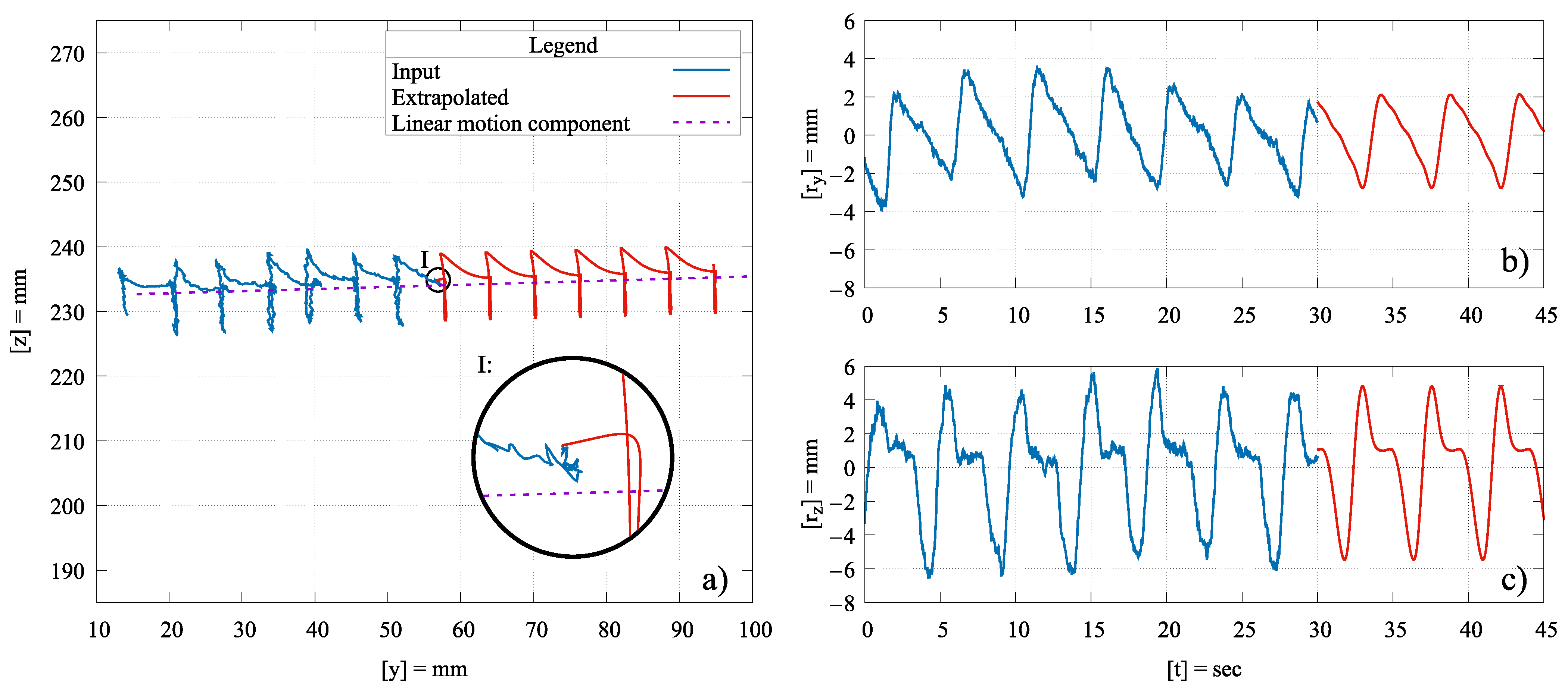
which is required for a smooth transition from the measurement to the extrapolation function, because Equations (7) and (9) are applied to determine the spline coefficients (the last and the first spline segments share a common sample point). Figure 5 shows the algorithm applied to the measured input signal (compare Figure 3) for spline sample points per residual motion period.
It can be seen that the choice of the number of sample points, as well as the amplitude adjustment by the median amplitude of the last 3 periods of the input signal, lead to a suitably fitting shape of the extrapolated signal. With all spline coefficients determined, Equation (19) can be calculated online for an unlimited period of time.
3.3. Resumption of the Control by the Input Device
At the point in time when the operator chooses to take back manual control, the relative translational motion with reference to the starting point of the input trajectory is added to the actual translatory position of the extrapolated signal directly. However, it turns out by practical experience that the rotational motion has to be blended in from the new input signal according to
( and , respectively), with used for tuning the blending speed. This allows the operator to adjust for orientation misalignment during the next motion patterns while the algorithm provides a continuous trajectory for the robot. When the orientation error is sufficiently small, i.e.,
is met for all orientation angles, the output is switched back to the input device again.
4. Experimental Validation
To validate the proposed extrapolation algorithm for its practical feasibility, single V-grooves were welded. The 8 mm metal sheets (EN 10025-2 material: S235JR + AR) were prepared with a 30-degree edge and were pre-positioned and tacked to each other. The seams to be welded were at least 150 mm (in length) and ranged up to 200 mm in length. All seams were welded in a flat position (ISO 6947: PA/ASME, Sec. IX: 1G) using a 1 mm diameter wire (ISO 14341-A: G42 4 M21 3Si1) and argon (ISO 14175: I1) as the shielding gas. The wire feed rate and the used current settings were varied over the tests. A trained and experienced welder operated the system. After welding a straight-line root seam, the top bead was used to activate the extrapolation algorithm and to resume manual control afterward to finish the weld seam. The operator performed the manual welding process of the top-bead for at least 30 s with a Christmas-tree-shaped hand motion before he activated the extrapolation algorithm. The extrapolation algorithm was applied for at least 30 s before resuming the manual control. The parameters of the equations used in the experiments are given in Table 1. Focus is put on the quality impact of the hand tremor suppression and if visible differences in the weld seam’s surface pattern occur, especially at the beginning of the extrapolation.
4.1. Input Device and Robot Working Cell Setup
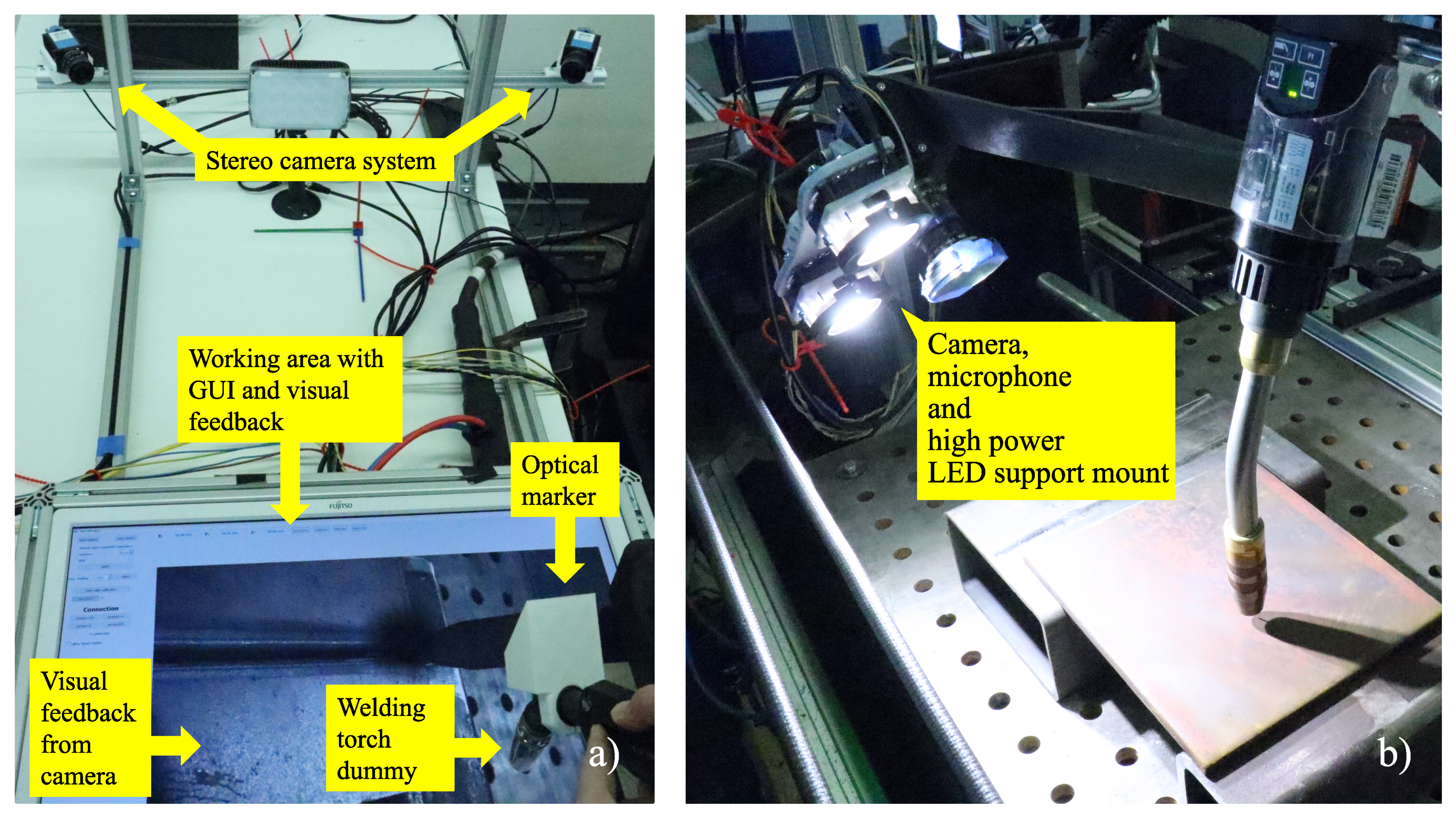
The experiments were carried out on a research setup for remote robot welding. To capture the hand-motion of the operator, a stereoscopic sensor system was used that consists of two DMK33GP2000e cameras [28], as can be seen in Figure 6a. During the welding process, visual information was provided to the operator from underneath a transparent ground plate by a computer display. The workspace provided a mm cube to operate in. The robot used is a KR6 Agilus R900, which was operated in the same room because the welding robot was mounted in an individual welding cell with an exhaust system and a height-adjustable protection glass. The workspace of the robot had a defined working plane of mm. To use different tools during system operation, a fully automated pneumatic tool-change process was integrated.
A modified welding-torch-gun was used as an input device, which was tracked optically utilizing an attached optical marker. The relative pose between the tool center point and the marker was referenced by a dedicated holder. Additionally, the orientation of the working plane of the robot was aligned to the input device’s coordinate system with a 2D laser scanner.
The interface to the robot for direct motion control, the KuKa RSI [29] module, demands a deterministic response of the trajectory generation module every 4 ms. Due to the non-deterministic image-data processing time and due to the Windows 10 operating system, which is needed to take the full advantage of the used cameras, hard real-time cannot be achieved. Furthermore, the cameras of the stereoscopic vision system operate with a framerate of Hz. Therefore, the quantized data from the stereoscopic system must be either filtered by a second-order linear filter or shaped into a two-times continuously differentiable trajectory by other means. In the paper [30] the authors propose and validate an interpolation algorithm consisting of a linear Kalman filter and a PT-2 error observer, which generates an appropriate trajectory with low latency. This algorithm is calculated on a dedicated real-time PC running Linux with the PREEMPT_RT [31] patch and the resulting trajectory was used as the input signal to the extrapolation algorithm covered in this paper.
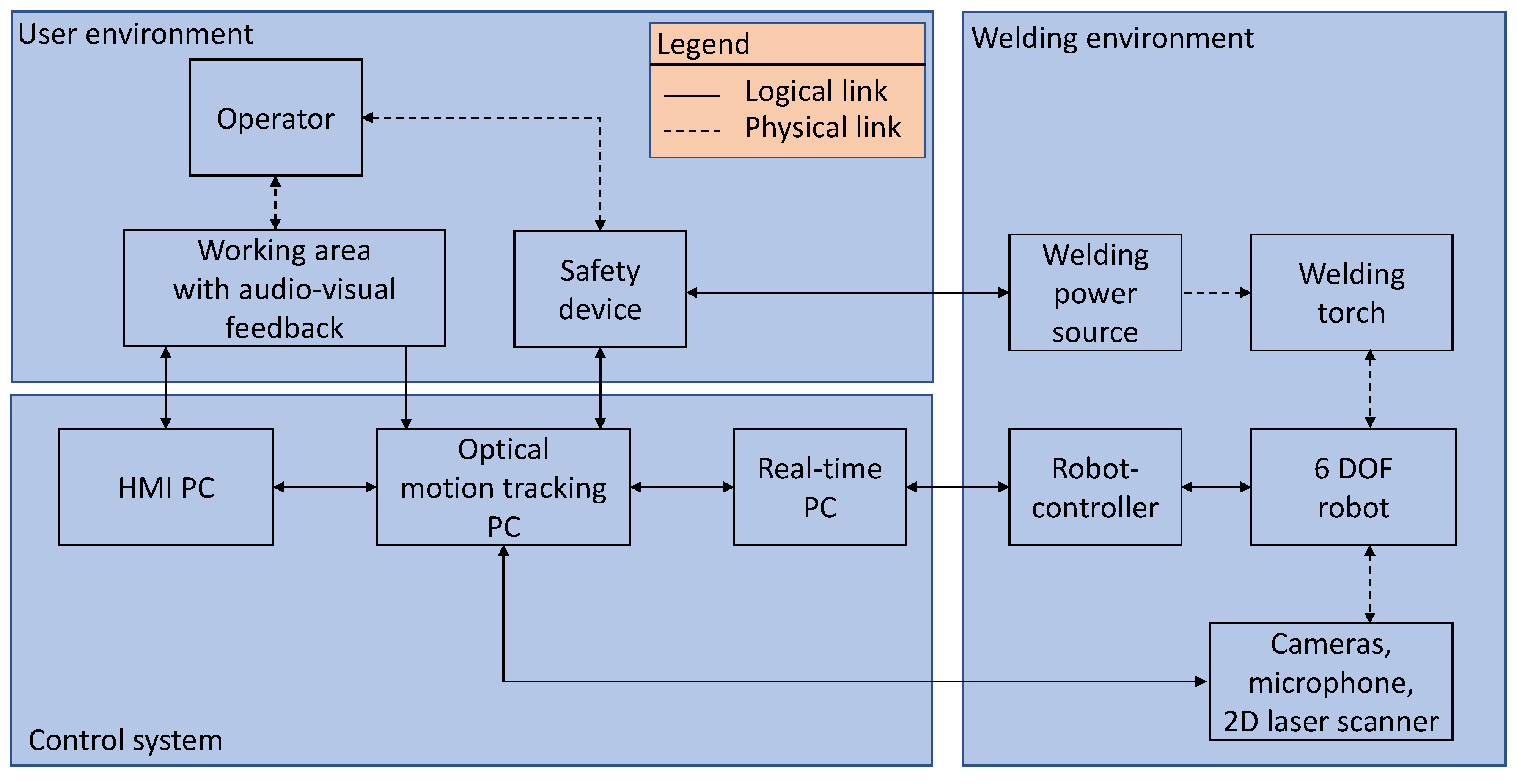
A footswitch was used to activate the extrapolation algorithm and to resume the manual control of the robot again afterward. Figure 7 gives an overview of the complete system.
4.2. Results
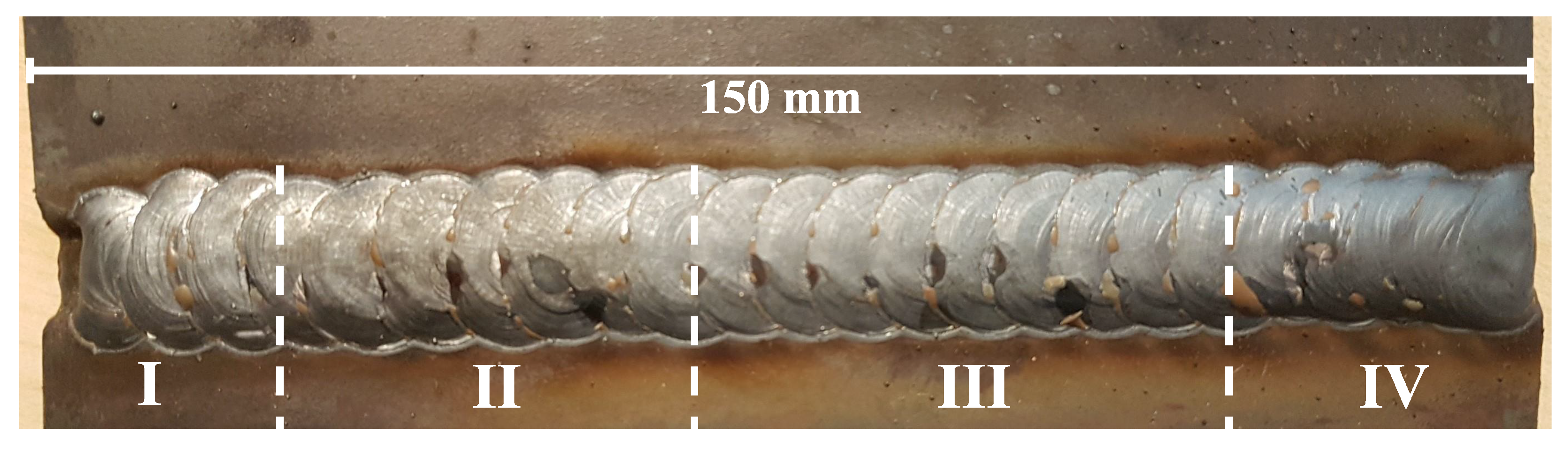
Figure 8 shows a selected representative result from the tests. Section 1 marks the area in which the operator started the seam. He ignited the arc and created the required fused material. Furthermore, the Christmas tree motion pattern was initiated visibly by the structure of the bead. The variations in the seam’s outer geometry and in the motion pattern show the adjustment process of the operator in order to achieve a proper and sound result. After a short period of time, the welder mastered the required motion and traveling speed and entered Section 2, where he continued the seam in steady-state periodic motion. Overall, the process (Section 1 and Section 2) took 44 s with a length of 60 mm.
At the end of Section 2, the extrapolation algorithm was activated and was deactivated again at the end of Section 3. Section 1 had a total length of 60 mm and the algorithm presented in this article was activated for 41.2 s to complete it. During this period, the operator could relax, oversee the welding by the robot and reposition his dummy welding torch in the working area. Deviations in the outer geometric dimensions of the seam are not recognizable without closer examination. The fused mass in combination with the extrapolation algorithm created a homogeneous weld seam. At the beginning of Section 4, the control was resumed by the operator at the holding position of the Christmas-tree-shaped motion pattern. Section 4 was 28 mm long and small differences in the seam’s outer geometric dimensions can be seen.
4.3. Discussion
The results show the performance of the presented algorithm. Without close visual inspection, a changeover from the manually performed weld to the extrapolation algorithm is not detectable. The extrapolated section of the weld is only distinguishable by its precise periodic pattern. Process parameters, such as the feed-wire rate and the flow rate of the protection gas, can be kept constant over the whole process.
The spline resembles the geometric motion pattern as well as the motion speed adequately because the visual properties of the weld do not change. The choice that the seam width is determined by the median of the extreme values of the last three periods of the input signal leads to the best outer geometry fidelity. When the number of motion periods considered is decreased, the results become too prone to geometric mistakes by the operator, which cause falsely estimated dimensions for the algorithm. Inclusion of all motion periods captured in the data set can also lead to inferior results because on some occasions the operator has to cover up small welding errors. That would mean that the operator would have to weld for 30 s close to perfection before the extrapolation algorithm could be activated. With the described solution, the operator can judge the quality of the last three periods and activate the extrapolation accordingly. When averaging instead of the median filter is used, the outer geometry fidelity decreases, because the influence of the hand-tremor is too strong.
The choice of 10 spline nodes is a good trade-off between geometric fidelity and tremor suppression. However, the optical impression of a sound weld seam is prone to subjective judgment. As a result, this parameter was tuned with the help of an experienced welder, who gave feedback on what geometric shape he intended to achieve. Fewer nodes decrease the alignment of the spline to the original signal. Simulation yields that 5 nodes are the minimum required for the reconstruction of the original signal. The variance of the error decreases strongly with an increased number of nodes until reaching 10 nodes. More nodes will further decrease the variance in small amounts but the acquisition of the tremor increases, which results in undesired spiky spline segments. The optical impression of a sound weld seam is prone to subjective judgment. As a result, we tuned this parameter with the help of an experienced welder.
The motion speed was kept adequately as well because no heightening or thinning of the seam can be observed. However, at the beginning of Section 4 a heightening frequently occurs since the operator has to resume the motion pattern and speed without aid. The filtered resumption of the orientation according to Equation (21) allows the operator to concentrate on the translatory motion first. The experiments show that this needs to be trained by the welder and leads to improved results over time. The result depicted in Figure 8 was obtained after the 5th try by an experienced welder and was the first he was satisfied with. Further aiding by visual guides on the GUI can be provided but is regarded as distracting by that particular welder. It is not possible to judge from the motion signal alone if a weld is successful or not.
To evaluate, if the signal contains periodic characteristics, the recorded manual input signal is freed from affine linear components by Equation (2) and examined by its standard deviation. Periodic signals differ strongly from tremor-loaded lines. The welder who performed the experiments showed a typical hand tremor of 2.5 mm. With an appropriate margin, the threshold was set to 3.0 mm. It is easily adjustable to any operator but proved to be an appropriate value for untrained users as well.
The pose of the welding torch (orientation and distance to the y-z-plane) in Section 2 of the discussed result was close to constant due to the trained operator’s skill. To freeze these values during the active extrapolation algorithm is important to create sufficient results. However, a referencing of this plane by the 2D laser scanner is required. If structures such as corrugated sheet metal or spherical objects such as pipes require the inclusion of the x-axis, the algorithm can easily be extended, since the motion axes are analyzed individually and decoupled from each other. However, for spherical objects, a circular component has to be added to Equation (19).
5. Conclusions and Future Work
A computationally efficient extrapolation algorithm for manual remote welding has been presented. It was experimentally validated as applicable for straight-line, weaving, and Christmas-tree-shaped motion patterns. Because of the spline approach, it is able to provide motion patterns that better resemble the geometry of a Christmas-tree-shaped weld than those based on the composition of sine-templates as proposed by the authors of the paper [20]. The base frequency estimation by using a sampled autocorrelation function proved to be suitable as well.
The experimental proof-of-concept for extrapolation, re-positioning of the input device, and subsequent resumption of control to overcome the spatial limitations of a geometrical input device was given. The experiments revealed that even long distances can be welded by the presented algorithm as long as the overall linear direction remains constant. Moreover, there is no theoretical limitation to the extrapolation length, as long as the material properties do not change. The operator is allowed to relax, supervise the process and occasionally resume manual control to adjust the overall direction or the motion pattern and then hand the control over to the algorithm again. This leads to substantial relief of strain from the operator.
A trained and experienced operator has assessed the weld quality of the samples as promising. As a result, in the near future, a metallography analysis of the weld seam will be performed to ensure that the extrapolation of the inner geometry leads to flawless welds. Afterward, a certification for the system for professional welding operations will be pursued. An improved input device and a dedicated robot tool are currently in fabrication. An extension of the algorithm incorporating distance control and an online adaptation of the overall direction during extrapolation are being considered for future work.
Author Contributions
Conceptualization, L.C.E., P.Z. and J.M.; methodology, L.C.E., P.Z. and J.M.; software, L.C.E. and P.Z.; validation, L.C.E. and P.Z.; writing—original draft preparation, L.C.E., P.Z. and J.M.; writing—review and editing, J.M. and S.S.; visualization, L.C.E. and J.M.; supervision, S.S. and J.M.; funding acquisition, S.S. All authors have read and agreed to the published version of the manuscript.
Funding
Funded by Hamburgerische Investitions-und Förderbank (IFB Hamburg) within the scope of the European Regional Development Fund, grant number: 51086029.
Institutional Review Board Statement
Not applicable.
Informed Consent Statement
Not applicable.
Acknowledgments
This work is part of the research project MeRItec.
Conflicts of Interest
The authors declare no conflict of interest. The funders had no role in the design of the study; in the collection, analyses, or interpretation of data; in the writing of the manuscript, or in the decision to publish the results.
Abbreviations
The following abbreviations are used in this manuscript:
| VR | Virtual reality |
| KUKA | Keller und Knappich Augsburg |
| RMS | Root of mean squares value |
| ACF | Autocorrelation function |
| GUI | Graphical user interface |
References
- Papakostas, N.; Alexopoulos, K.; Kopanakis, A. Integrating digital manufacturing and simulation tools in the assembly design process: A cooperating robots cell case. CIRP J. Manuf. Sci. Technol. 2011, 4, 96–100. [Google Scholar] [CrossRef]
- Papakostasa, N.; Pintzos, G.; Matsas, M.; Chryssolouris, G. Knowledge-enabled design of cooperating robots assembly cells. Procidia CIRP 2014, 23, 165–170. [Google Scholar] [CrossRef] [Green Version]
- Pellegrinelli, S.; Pedrocchi, N.; Tosatti, L.M.; Fischer, A.; Tolio, T. Multi-robot spot-welding cells: An integrated approach to cell design and motion planning. CIRP Ann. 2014, 63, 17–20. [Google Scholar] [CrossRef] [Green Version]
- Pellegrinelli, S.; Pedrocchi, N.; Tosatti, L.M.; Fischer, A.; Tolio, T. Validation of an extended approach to multi-robot cell design and motion planning. Procedia CIRP 2015, 36, 6–11. [Google Scholar] [CrossRef] [Green Version]
- Bartelt, M.; Stumm, S.; Kuhlenkoetter, B. Tool oriented Robot Cooperation. Procedia CIRP 2014, 23, 188–193. [Google Scholar] [CrossRef] [Green Version]
- Ong, S.K.; Nee, A.Y.C.; Yew, A.W.W.; Thanigaivel, N.K. AR-assisted robot welding programming. Adv. Manuf. 2020, 8, 40–48. [Google Scholar] [CrossRef]
- Brosque, C.; Galbally, E.; Khatib, O.; Fischer, M. Human-Robot Collaboration in Construction: Opportunities and Challenges. In Proceedings of the International Congress on Human-Computer Interaction, Optimization and Robotic Applications (HORA), Ankara, Turkey, 26–28 June 2020; pp. 1–8. [Google Scholar]
- Dianatfar, M.; Latokartano, J.; Lanz, M. Review on existing VR/AR solutions in human-robot collaboration. Procedia CIRP 2021, 97, 407–411. [Google Scholar] [CrossRef]
- Wang, Q.; Jiao, W.; Yu, R.; Johnson, M.T.; Zha, Y. Modeling of Human Welders’ Operations in Virtual Reality Human-Robot Interaction. IEEE Robot. Autom. Lett. 2019, 10, 2958–2964. [Google Scholar]
- Wang, Q.; Jiao, W.; Yu, R.; Johnson, M.T.; Zhang, Y. Virtual reality robot-assisted welding based on human intention recognition. IEEE Trans. Autom. Sci. Eng. 2020, 17, 799–808. [Google Scholar] [CrossRef]
- Liu, Y.; Zhang, Y.M. Control of human arm movement in machine-human cooperative welding process. Control Eng. Pract. 2014, 32, 161–171. [Google Scholar] [CrossRef]
- Liu, Y.; Zhang, Y. Toward welding robot with human knowledge: A remotely-controlled approach. IEEE Trans. Autom. Sci. Eng. 2015, 12, 769–774. [Google Scholar] [CrossRef]
- Xu, J.; Zhang, G.; Hou, Z.; Wang, J.; Liang, J.; Bao, X.; Yang, W.; Wang, W. Advances in multi-robotic welding techniques: A review. Int. J. Mech. Eng. Robot. Res. 2020, 9, 421–428. [Google Scholar] [CrossRef]
- Dharmawan, A.G.; Vibhute, A.A.; Foong, S.; Soh, G.S.; Otto, K. 3D reconstruction of complex spatial weld seam for autonomous welding by laser structured light scanning. J. Manuf. Process. 2019, 39, 200–207. [Google Scholar]
- Shah, H.N.M.; Sulaiman, M.; Shukor, A.Z.; Rashid, M.Z.A.; Jamaluddin, M.H. A review paper on vision based identification, detection and tracking of weld seams path in welding robot environment. Mod. Appl. Sci. 2019, 10, 83–89. [Google Scholar] [CrossRef] [Green Version]
- Ding, Y.; Huang, W.; Kovacevic, R. An on-line shape-matching weld seam tracking system. Robot. Comput. Integr. Manuf. 2016, 42, 103–112. [Google Scholar] [CrossRef]
- Li, X.; Li, X.; Ge, S.S.; Khyam, M.O.; Luo, C. Automatic welding seam tracking and identification. IEEE Trans. Ind. Electron. 2017, 64, 7261–7271. [Google Scholar] [CrossRef]
- Zhang, K.; Yan, M.; Huang, T.; Zheng, J.; Li, Z. A Survey of Platform Designs for Portable Robotic Welding in Large Scale Structures. J. Manuf. Process. 2019, 39, 200–207. [Google Scholar] [CrossRef]
- Norberto Pires, J.; Loureiro, A.; Bolmsjö, G. Welding Robots: Technology, System Issues and Applications; Springer: London, UK, 2006; ISBN 13: 978–1852339531. [Google Scholar]
- Eto, H.; Asada, H.H. Seamless manual-to-autopilot transition: An intuitive programming approach to robotic welding. In Proceedings of the 8th IEEE International Conference on Robot and Human Interactive Communication, New Delhi, India, 14–18 October 2019; pp. 1–7. [Google Scholar] [CrossRef]
- Marlow, F.M. Welding Know-How, 1st ed.; Metal Arts Press: Huntington Beach, CA, USA, 2012; ISBN 13 978-0-9759963-6-2. [Google Scholar]
- Erden, M.S.; Billard, A. Hand impedance measurements during interactive manual welding with a robot. IEEE Trans. Robot. 2015, 31, 168–179. [Google Scholar] [CrossRef]
- Erden, M.S.; Billard, A. Robotic assistance by impedance compensation for hand movements while manual welding. IEEE Trans. Cybern. 2016, 46, 2459–2472. [Google Scholar] [CrossRef]
- van Essen, J.; van der Jagt, M.; Troll, N.; Wanders, M.; Erden, M.S.; van Beek, T.; Tomiyama, T. Identifying Welding Skills for Robot Assistance. In Proceedings of the IEEE/ASME International Conference on Mechtronic and Embedded Systems and Applications, Beijing, China, 12–15 October 2008; pp. 437–442. [Google Scholar] [CrossRef]
- Erden, M.S. Manual Welding with Robotic Assistance Compared to Conventional Manual Welding. In Proceedings of the IEEE 14th International Conference on Automation Science and Engineering (CASE), Munich, Germany, 20–24 August 2018; pp. 570–573. [Google Scholar]
- Sanderson, C.; Curtin, R. Armadillo: A template-based C++ library for linear algebra. J. Open Source Softw. 2016, 1, 26. [Google Scholar] [CrossRef]
- Sanderson, C.; Curtin, R. An adaptive solver for systems of linear equations. In Proceedings of the 14th International Conference on Signal Processing and Communication Systems (ICSPCS), Adelaide, Australia, 14–16 December 2020; pp. 1–6. [Google Scholar] [CrossRef]
- DMK33GP2000e. Available online: https://www.theimagingsource.com/products/industrial-cameras/gige-monochrome/dmk33gp2000e/ (accessed on 13 May 2021).
- KUKA RSI. Available online: https://www.kuka.com/en-gb/services/downloads?terms=Language:en: (accessed on 13 May 2021).
- Ebel, L.C.; Zuther, P.; Maass, J.; Sheikhi, S. Motion signal processing for a remote gas metal arc welding application. Robotics 2020, 9, 30. [Google Scholar] [CrossRef]
- The Linux Foundation. Available online: https://wiki.linuxfoundation.org/realtime/start (accessed on 13 May 2021).
Figure 1.
Dealing with a limited input device tracking area. (a) Motion controlled by input device tracking, (b) motion controlled by extrapolation of the input signal while the operator re-configures the input device pose, (c) resumption of the motion control by input device tracking.
Figure 1.
Dealing with a limited input device tracking area. (a) Motion controlled by input device tracking, (b) motion controlled by extrapolation of the input signal while the operator re-configures the input device pose, (c) resumption of the motion control by input device tracking.

Figure 2.
Input coordinate system and definition of the rotation angles. The red coordinate system marks the origin of the workspace.
Figure 2.
Input coordinate system and definition of the rotation angles. The red coordinate system marks the origin of the workspace.

Figure 3.
Measured motion pattern for a Christmas-tree-shaped weld. (a) Path in the y-z-plane showing a periodic motion and hand tremor, (b,c) signals over time showing the linear and periodic motion components.
Figure 3.
Measured motion pattern for a Christmas-tree-shaped weld. (a) Path in the y-z-plane showing a periodic motion and hand tremor, (b,c) signals over time showing the linear and periodic motion components.

Figure 4.
Autocorrelation signals of the welding motion.

Figure 5.
Functioning of the algorithm. (a) Extrapolated path with the linear component added according to Equation (19), detail I showing the effect of the blending term , (b,c) resemblance of the residual periodic motion , by a spline function showing the matching of the shapes.
Figure 5.
Functioning of the algorithm. (a) Extrapolated path with the linear component added according to Equation (19), detail I showing the effect of the blending term , (b,c) resemblance of the residual periodic motion , by a spline function showing the matching of the shapes.

Figure 6.
Experimental setup. (a) Input device and GUI with audio-visual feedback, (b) workspace of the welding robot.
Figure 6.
Experimental setup. (a) Input device and GUI with audio-visual feedback, (b) workspace of the welding robot.

Figure 7.
System overview of the experimental setup showing the signal flows.

Figure 8.
Successful extrapolation of a weld seam with a Christmas-tree-shaped pattern. Section I: starting welding process and seam motion pattern; Section II: steady-state periodic motion; Section III: extrapolation algorithm applied successfully; Section IV: resumption of control by the operator.


Table 1.
Values used in experimental validation.
| Variable | Symbol | Value |
|---|---|---|
| Sample time | T | s |
| Spline supporting points | n | 10 |
| ACF horizon | m | 2000 Samples |
| Orientation error threshold | ||
| Decay (translational blending) | ||
| Blending coefficient (rotational) |
Publisher’s Note: MDPI stays neutral with regard to jurisdictional claims in published maps and institutional affiliations. |
© 2021 by the authors. Licensee MDPI, Basel, Switzerland. This article is an open access article distributed under the terms and conditions of the Creative Commons Attribution (CC BY) license (https://creativecommons.org/licenses/by/4.0/).
Share and Cite
MDPI and ACS Style
Ebel, L.C.; Maaß, J.; Zuther, P.; Sheikhi, S. Trajectory Extrapolation for Manual Robot Remote Welding. Robotics 2021, 10, 77. https://0-doi-org.brum.beds.ac.uk/10.3390/robotics10020077
AMA Style
Ebel LC, Maaß J, Zuther P, Sheikhi S. Trajectory Extrapolation for Manual Robot Remote Welding. Robotics. 2021; 10(2):77. https://0-doi-org.brum.beds.ac.uk/10.3390/robotics10020077
Chicago/Turabian StyleEbel, Lucas Christoph, Jochen Maaß, Patrick Zuther, and Shahram Sheikhi. 2021. "Trajectory Extrapolation for Manual Robot Remote Welding" Robotics 10, no. 2: 77. https://0-doi-org.brum.beds.ac.uk/10.3390/robotics10020077
Note that from the first issue of 2016, this journal uses article numbers instead of page numbers. See further details here.