On the Modelling of Tethered Mobile Robots as Redundant Manipulators

Abstract

Controlling a chain of tethered mobile robots (TMRs) can be a challenging task. This kind of system can be considered kinematically as an open-chain robotic arm where the mobile robots are considered as a revolute joint and the tether is considered as a variable length link, using a prismatic joint. Thus, the TMRs problem is decoupled into two parallel problems: the equivalent robotic manipulator control and the tether shape computation. Kinematic redundancy is exploited in order to coordinate the motion of all mobile robots forming the chain, expressing the constraints acting on the mobile robots as secondary tasks for the equivalent robotic arm. Implementation in the Gazebo simulation environment shows that the methodology is capable of controlling the chain of TMRs in cluttered environments.

1. Introduction

Since the early beginnings of mobile robotics, one of the key aspects of these systems was that of autonomy, both from a decision-making perspective, as well as from a physical one. This meant that, in the most general definition, a mobile robot should be physically unlinked from the environment or from other fixed devices. The direct consequence of this was the development and implementation of state-of-the-art energy accumulation systems, e.g., batteries, tele-control or autonomous on-board decision-making [1].

This being said, there are a set of specific cases where a physical link is unavoidable or at least exceedingly desirable:

• High-power/consumption applications, e.g., welding applications, long-duration and perpetual drone flight,
• Exploration of environments which prevent tele-control, e.g., caves, tunnels or mines, underwater environments,
• Transfer of matter from a base station to the robot, e.g., the transfer of paint and compressed air in robotized painting applications.

Although single tethered mobile robot (TMR) has been widely covered in literature, here we focus on multi-robot systems, such as: platoons [2] and trains of robots connected by cables [3,4,5]. The former concerns parallel arrangements of TMRs, and the latter regards serial arrangements or chains of mobile robots.

Using more than one mobile robot in a system forming a chain drastically increases the working space and the manoeuvrability. Previous works on this kind of system considered mainly aspects related to control and generally lacked an explicit kinematic formulation. Here, we propose a formal way to handle the kinematics of this kind of systems by treating a chain of TMRs as a serial open-chain robotic manipulator. Each mobile robot is thus represented by a revolute joint and the cable is considered as a prismatic joint. In the following, we will refer to the fixed attachment point of the chain as the base, the leading robot also as the end-effector and the robots in between as the intermediate robots.

Formally, when the number of mobile robots is two or more, the equivalent robotic manipulator becomes a redundant system. This equivalence allows us to exploit the inverse kinematics (IK) solution of redundant manipulators (RMs) to solve the problem. In this regard, constraints on the mobile robots kinematics are expressed as secondary tasks for the equivalent RM. For example, one of these constraints is the influence of the tether which must avoid touching the ground.

The present work arose from a specific industrial request about painting applications with robots very large objects, for example, small airplanes or boats. In this case, the robotics arm, used for painting, must be able to move around in an environment where the objects are not positioned with extreme precision. Robotized painting presents two main problems: the first is that it is an extremely power demanding task, which obviously cannot be performed by using only batteries; the second is that the environment is going to be harsh and operators cannot be present inside the working area. Another important application of chains of TMRs in this context is about pressure washing. In this specific case, cables must provide both power supply but also water and detergent fluid. Given these requirements and limitations, the proposed solution is to use a mobile manipulator, powered with a cable line. However, since the manipulator has to cover a large area in order to perform the required task, a direct link from the wall to the mobile manipulator is highly undesirable. The mobile manipulator must be able to navigate around the object and, in this case, the cable would hit the obstacle or tangle. For this reason, and in order to increase the manoeuvrability of the overall system, the choice of using multiple mobile robots in series is considered. The intermediate robots have the task of acting as a fairlead and of rearranging the configuration of the cables in the workspace. Nevertheless, the introduction of cables in the environment greatly complicates planning and control, and their management during the whole motion of the system.

We acknowledge that there exists a general lack of explicit kinematic formulations in literature in the field of chains of TMRs; more specifically, most contributions are limited to control theory aspects. The present work aims at tackling the industrial problem while providing a general framework in which TMRs are modeled as redundant manipulators in an exhaustive and formally elegant way.

The integration of the cable is especially straightforward within this framework; it allows a catenary-based description of the cable, thus breaking away from the limiting taut cables hypothesis while at the same time being able to compute tension forces and implement constraints on the kinematics of the robots. By assimilating the cable to a manipulator link, it is possible through appropriate methods to constrain the cable to not touch the ground and always have an elongation within a certain range. Moreover, the reconfiguration of the cable in the environment is achievable in a convenient way through the classic obstacle avoidance for manipulators. The ability to avoid hitting the ground with the cable and not to tangle somewhere in the environment granted by this approach makes the problem of planning easier. Finally, the framework allows the system of tethered robots to be easily expanded to the case of n robots by iteration.

In order to fully characterize our framework, a sensitivity analysis was performed on its main parameters, highlighting the advantages and drawbacks of the methodology.

In order to validate our results, we elected to exploit the Gazebo dynamics simulator for the motion of the robots; this allowed us to have complete control on the environment, thus helping exclude exogenous error sources linked to the non-structured, real environments.

The paper is structured as follows: in Section 2, a detailed analysis is presented of the state-of-the-art in both the field of tethered and RMs. In Section 3, the kinematic analogy is illustrated between a chain of TMRs and an RM from a general point of view. In Section 4, the case studies are presented, which consist of three omnidirectional mobile robots connected in an open chain and traveling in four different scenarios: three ideal, one related to the industrial painting task of a small plane. In Section 5, results are shown and discussed. One ideal use case and the industrial one are compared with simulations in Gazebo for validation. In the same section, the sensitivity analysis results are shown the plane case study. Finally, in the Conclusions, we highlight the main aspects of the implementation and the related results, and discuss possible future research in this direction.

2. Related Works

In the following, the two main aspects of the state-of-the-art are discussed that are relevant to the work we put forth in the following sections: tethered robots, and frameworks for solving robot redundancies.

2.1. Tethered Robots

In applications where robots have large power demands, tethers are a welcome feature; tethers are also widely used for data, communication and control in applications that require extremely high degrees of reliability. A chief example is the case of underwater robotics [6] ROVs (Remotely Operated Vehicles) since wireless communications with the ship through water is often impracticable. Literature shows application in matter transfer, e.g., for fluids [1], for traction support and assisting mobile robot on climbing steep slopes [7,8,9,10], for robotized tank inspection [11] and also for towing objects on the ground [12] and in the air [13,14,15]. They are also used in Urban Search and Rescue (USAR) [1] as well as in Unmanned Aerial Vehicles (UAVs) [16] and found use also in mobile CDPRs (Cable-Driven Parallel Robots) [17].

Fukushima et al. in 2001 studied TMRs which implemented a model of the cable called ’hyper-tether’. This methodology allows for actively controlling the tether tension and length [18]. Later, in 2014, the issue of the navigation of a TMR was tackled by Kim et al., which developed a topological method based on the homotopy class of the cable [19]. More recently, in 2015, Kim and Likhachev studied the path planning of a TMR problem using a multi-heuristic A* algorithm approach [20].

TMRs have found use in space applications, e.g., for the rovers Nanokhod [1] and the ESA ROSA MicroRover [21], where mission constraints about dimensions and mass of the rovers are prohibitive for a completely autonomous system.

While in literature a large amount of work exists on a single mobile robot connected by a tether to a fixed point, few examples exist about chains of TMRs. Fagiano proposes a model to control a chain of UAV multicopters connected with each other by flexible tethers [3]; Tognon et al. discussed two tethered multicopters connected with a base, and considered the system as a two degrees of freedom planar arm [4]; Kosarnovsky considers an undefined number of UAVs as a robotic arm [5].

2.2. Approaches towards Robot Redundancy

The fact that the IK for an RM allows for infinite solutions has the advantage that redundancy can be exploited to either execute other tasks or to apply additional constraints. The main methods to solve this redundant kinematics while satisfying these additional constraints are: the Extended Jacobian (EJ) approach [22], the Task Space Augmentation (TSA) [23,24], the Task Priority (TP) approach and the Gradient Projection Method (GPM).

Both EJ and TSA aim at including the constraints in the Jacobian, increasing its size. These methods differ on how the constraints are expressed, and the IK solution is obtained by inverting the new Jacobian. Both methods are subjected to algorithm singularities. In fact, by increasing the number of tasks, the likelihood of a singularity condition increases. In particular, the Jacobian becomes singular even if the single task Jacobians are full rank [25]. Later, Simas et al. proposed a method to adapt the coefficients describing the constraints included in the EJ in order to keep the robot far from singularities [26].

In order to handle these situations, the TP approach was first proposed by Nakamura et al. [27] and Maciejewski et al. [28] for two tasks and later extended in a general way by Sciavicco et al. to the case of t tasks [29]. Despite this, the method is subject to algorithm singularity [25], which can be overcome by using a similar formulation proposed by Chiaverini [30,31], which is more robust near singularities, at the cost of greater tracking error for secondary tasks. Baerlocher et al. [32] extended this method to the case of t tasks. Finally, GPM [33,34] is a method in which the joint variables are computed in a way that maximizes an objective function; internal motion of the structure is then obtained by projecting the vector into the null space of the end-effector Jacobian.

Techniques developed for typical RM have been used for platooning problems and formation control [35,36,37]. Other works from Antonelli et al. [38,39] built on previous work by using singularity robust task priority [30,31] in order to prevent task conflicts.

In general, previous works operate by computing the Jacobians in the task space with respect to the robot’s position. Conversely, in this paper, we control a virtual RM explicitly; the Jacobians are thus computed with respect to its joint variables. In other words, we control a virtual RM in the joint space, while the positions of the mobile robots are mapped by exploiting the manipulator direct kinematics.

3. Methodology

Let us consider a chain composed by a set of n mobile robots arranged in three-dimensional space, such that the first one is tethered to a fixed point (e.g., the ground, a wall), and the others are connected between them such that they form an open chain. The position of each robot is then defined by a vector ${\mathit{x}}_{\mathit{k}}\in {\mathbb{R}}^3$ with $k=1,\cdots ,n$. Since the robots are tethered, this leads to the fact that the robot k depends on the previous robot, i.e., ${\mathit{x}}_{\mathit{k}}=f\left({\mathit{x}}_{\mathit{k}-\mathbf{1}}\right)$.

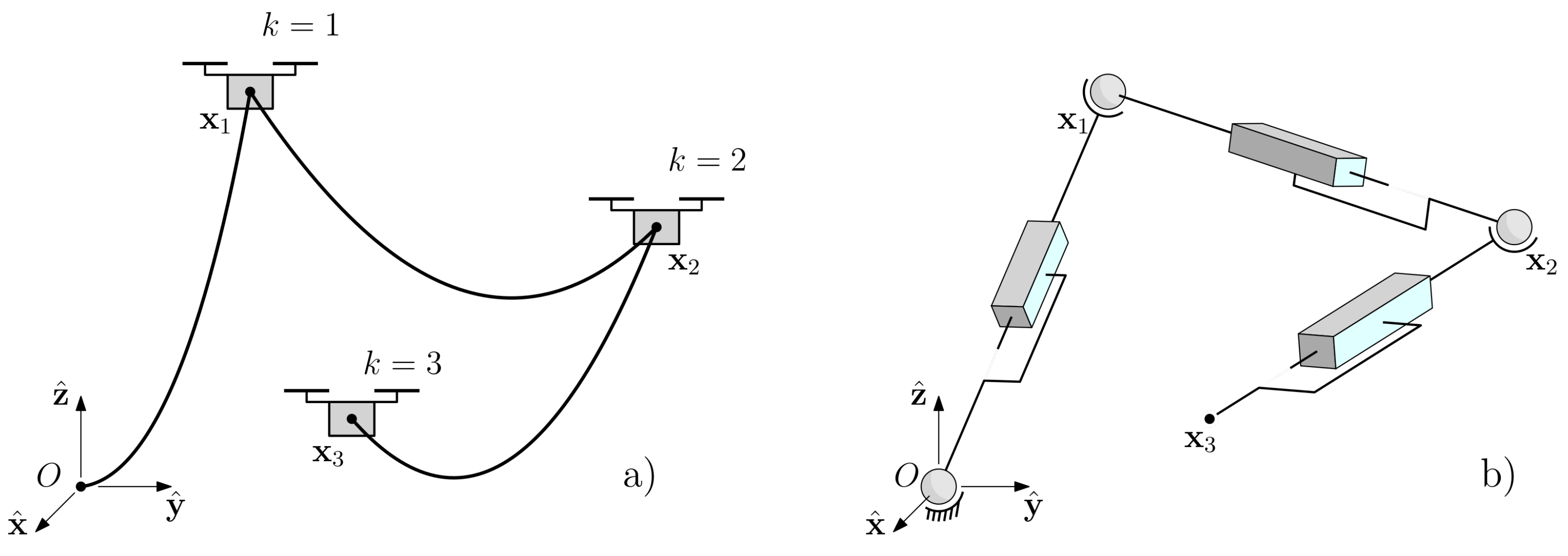
The analogy consists of considering each robot as a spherical joint, and the tether connecting two consecutive robots as a prismatic joint, as shown in Figure 1; at the same time, the tether shape can be solved as a parallel problem. The spherical joints have 2 Degrees of Freedom (DOFs) since the cable is assumed non-rotating. As such, the chain of TMRs can be considered kinematically as an open-chain manipulator; it is then possible to solve the n TMRs problem with the already known techniques used for manipulators.

Moreover, the joint variables are expressed according to the Denavit–Hartenberg (D–H) convention. It is thus possible to write the transformation matrix ${\mathit{T}}_{\mathit{i}}^{\mathit{i}-\mathbf{1}}$ between two consecutive joints, named i and $i-1$, as follows:

$${\mathit{T}}_{\mathit{i}}^{\mathit{i}-\mathbf{1}}=\left[\begin{array}{cccc}c{\vartheta }_i& -s{\vartheta }_{i}c{\alpha }_i& s{\vartheta }_{i}s{\alpha }_i& a_{i}c{\vartheta }_i\\ s{\vartheta }_i& c{\vartheta }_{i}c{\alpha }_i& -c{\vartheta }_{i}s{\alpha }_i& a_{i}s{\vartheta }_i\\ 0& s{\alpha }_i& c{\alpha }_i& d_i\\ 0& 0& 0& 1\end{array}\right]$$

(1)

where s and c denote, respectively, the sine and cosine functions, $d_i$ are prismatic and ${\vartheta }_i$ revolute joint variables.

Hence, between each robot, there are three active joints; by denoting as ${\mathit{T}}_{\mathit{i},\mathit{j}}^{\mathit{i}-\mathit{1},\mathit{j}}$ the homogeneous transformation between two consecutive joints i and $i-1$ along the j-th link connecting the two mobile robots, the position of the k-th robot, with respect to the base frame, is expressed as follows:

$${\mathit{x}}_{\mathit{k}}=\left[\begin{array}{cccc}1& 0& 0& 0\\ 0& 1& 0& 0\\ 0& 0& 1& 0\end{array}\right]\left(\prod _{j=1}^k\prod _{i=1}^3{T}_{i,j}^{i-1,j}\right){\left[\begin{array}{cccc}0& 0& 1& 0\end{array}\right]}^T$$

(2)

when $k=n$, then Equation (2) describes the direct kinematic function for the complete robotic manipulator and allows for mapping the end-effector pose in the task space given a joints vector $\mathit{q}$; in our case, this function allows us to map the mobile robots configuration. The direct kinematic function can be expressed in a more compact form as $\mathit{x}=k\left(\mathit{q}\right),$ where $k(·)$ is a nonlinear operator defined as $k:{\mathbb{R}}^n\to {\mathbb{R}}^m$, and $\mathit{q}\in {\mathbb{R}}^n$ is a vector composed by the joint variables.

Each introduced TMR increases the DOFs of the system by three: two for the spherical joint and one for the prismatic joint. In the 3D task space, to completely describe a given task 6-DOFs are needed: the position $(x,y,z)$ and the Euler angles $(\alpha ,\vartheta ,\phi )$ with respect to a fixed frame. If the task is only about positioning, then the DOFs required to fully define that task can be reduced to 3. This assumption can be done because we assume that the last robot, i.e., the end-effector, can rotate freely around its axis.

Let us consider the case where $n>1$: in this situation, the system is said to be redundant. It is thus possible to define the number of redundant DOFs, or Degrees of Redundancy (DORs) as $r=3(n-1)$. Given a pose, this system has ${\infty }^r$ solutions. Having a high number of DORs allows for the definition of a certain number of constraints or tasks which will have an influence on the behavior of the system.

Consider now the differential kinematics:

$$\dot{\mathit{x}}=\mathit{J}\left(\mathit{q}\right)\dot{\mathit{q}}$$

(3)

where $\dot{\mathit{x}}\in {\mathbb{R}}^m$ represents the task space velocities vector, and, in this case, $m=3$; $\dot{\mathit{q}}\in {\mathbb{R}}^n$ represents the joint space velocities vector, and $\mathit{J}\left(\mathit{q}\right)\in {\mathbb{R}}^{m\times n}$ is the Jacobian matrix; for redundant robots $\mathit{J},\left(\mathit{q}\right)$ is not squared since $m<n$. For a given task space velocities vector $\dot{\mathit{x}}$, the general solution of the inverse differential kinematics is expressed as follows:

$$\dot{\mathit{q}}={\mathit{J}}^{†}\left(\mathit{q}\right)\dot{\mathit{x}}+({\mathit{I}}_{\mathit{n}}+{\mathit{J}}^{†}\left(\mathit{q}\right)\mathit{J}\left(\mathit{q}\right)){\dot{\mathit{q}}}_{\mathbf{0}}$$

(4)

where ${\mathit{J}}^{†}\left(\mathit{q}\right)=\mathit{J}{\left(\mathit{q}\right)}^T{\left(\mathit{J}{\left(\mathit{q}\right)}^T\mathit{J}\left(\mathit{q}\right)\right)}^{-1}$ represents the Moore–Penrose pseudoinverse. For our purposes, we will not compute the above pseudoinverse since it is numerically unstable near the singularities. Instead, considering a very small constant $\lambda \in ]0,1[$, we will compute the pseudoinverse ${\mathit{J}}^{\#}\left(\mathit{q}\right)=\mathit{J}{\left(\mathit{q}\right)}^T(\mathit{J}{\left(\mathit{q}\right)}^T\mathit{J}\left(\mathit{q}\right)+\lambda {\mathit{I}}_{\mathit{n}})$ with the Damped Least Square Method, which is a trade-off between stability near singularities and a smoother output.

The first term in Equation (4) is the particular solution which solves Equation (3) in terms of least squares, while the second term is the homogeneous solution. The term $({\mathit{I}}_{\mathit{n}}+{\mathit{J}}^{†}\left(\mathit{q}\right)\mathit{J}\left(\mathit{q}\right))$ is an orthogonal projection operator which projects a generic vector $\dot{{\mathit{q}}_{\mathbf{0}}}$ into the null space $\mathcal{N}\left(\mathit{J}\right)$ of $\mathit{J}$.

In order to solve the IK for a RM, we use the formulation proposed by Chiaverini [30,31], more precisely its generalization to t tasks [32]. Within this formulation, the priorities are defined by $i=1,\cdots ,t$ where lower numbers indicate higher priorities and where ${\sum }_i^h{m}_i\le n$; the joint space velocity vector is defined as follows:

$$\dot{\mathit{q}}=\sum _{i=1}^t\left({\mathit{P}}_{\mathit{i}-\mathbf{1}}^{\mathit{A}}\left(\mathit{q}\right){{\mathit{J}}_{\mathit{i}}}^{\#}\left(\mathit{q}\right){\dot{\mathit{x}}}_{\mathit{i}}\right)+{\mathit{P}}_{\mathit{t}}^{\mathit{A}}\left(\mathit{q}\right){\dot{\mathit{q}}}_{\mathit{opt}}$$

(5)

where ${\mathit{P}}_{\mathit{i}}^{\mathit{A}}\left(\mathit{q}\right)=({\mathit{I}}_{\mathit{n}}-{\mathit{J}}_{\mathit{i}}^{{\mathit{A}}^{†}}\left(\mathit{q}\right){\mathit{J}}_{\mathit{i}}^{\mathit{A}}\left(\mathit{q}\right))$ denotes the projection operator into the null space of the Augmented Jacobian ${\mathit{J}}_{\mathit{i}}^{\mathit{A}}\left(\mathit{q}\right)$, which is in turn defined as follows:

$${\mathit{J}}_{\mathit{i}}^{\mathit{A}}\left(\mathit{q}\right)=\left[\begin{array}{c}{\mathit{J}}_{\mathbf{1}}\left(\mathit{q}\right)\\ ⋮\\ {\mathit{J}}_{\mathit{i}}\left(\mathit{q}\right)\end{array}\right]$$

(6)

Note that the projection operator ${\mathit{P}}_{\mathbf{0}}^{\mathit{A}}\left(\mathit{q}\right)={\mathit{I}}_{\mathit{n}}$ when $t=1$, i.e., the task is the primary one.

Let ${\dot{\mathit{x}}}_{\mathit{i}}$ be the i-th task velocity vector, and ${\mathit{J}}_{\mathit{i}}\left(\mathit{q}\right)$ the Jacobian associated with that task. Note that, in Equation (5), the joint optimization term ${\dot{\mathit{q}}}_{\mathit{opt}}$ has been explicitly defined. It is now possible to define a vector ${\mathit{q}}_{\mathit{opt}}$ such that it satisfies a certain constraint. Following the GPM, a typical choice is to specify the vector as a function of the gradient of an appropriate scalar objective function [33], which we call $w\left(\mathit{q}\right)$:

$${\dot{\mathit{q}}}_{\mathit{opt}}=k_0{\left(\frac{\partial w\left(\mathit{q}\right)}{\partial \mathit{q}}\right)}^T=k_0\nabla w\left(\mathit{q}\right)$$

(7)

where $k_0$ must be positive if the aim is the objective function $w\left(\mathit{q}\right)$ maximization.

By specifying the vector ${\dot{\mathit{q}}}_{\mathit{opt}}$, the generalization of Equation (3) can be used to express it in the task space velocities; subsequently, by substituting it in Equation (5), the task priority framework can be used. In this case, the primary task is being executed (usually the end-effector tracking a reference trajectory), and sub-tasks are executed in such a way that they do not interfere with the higher priority tasks.

4. Case Study

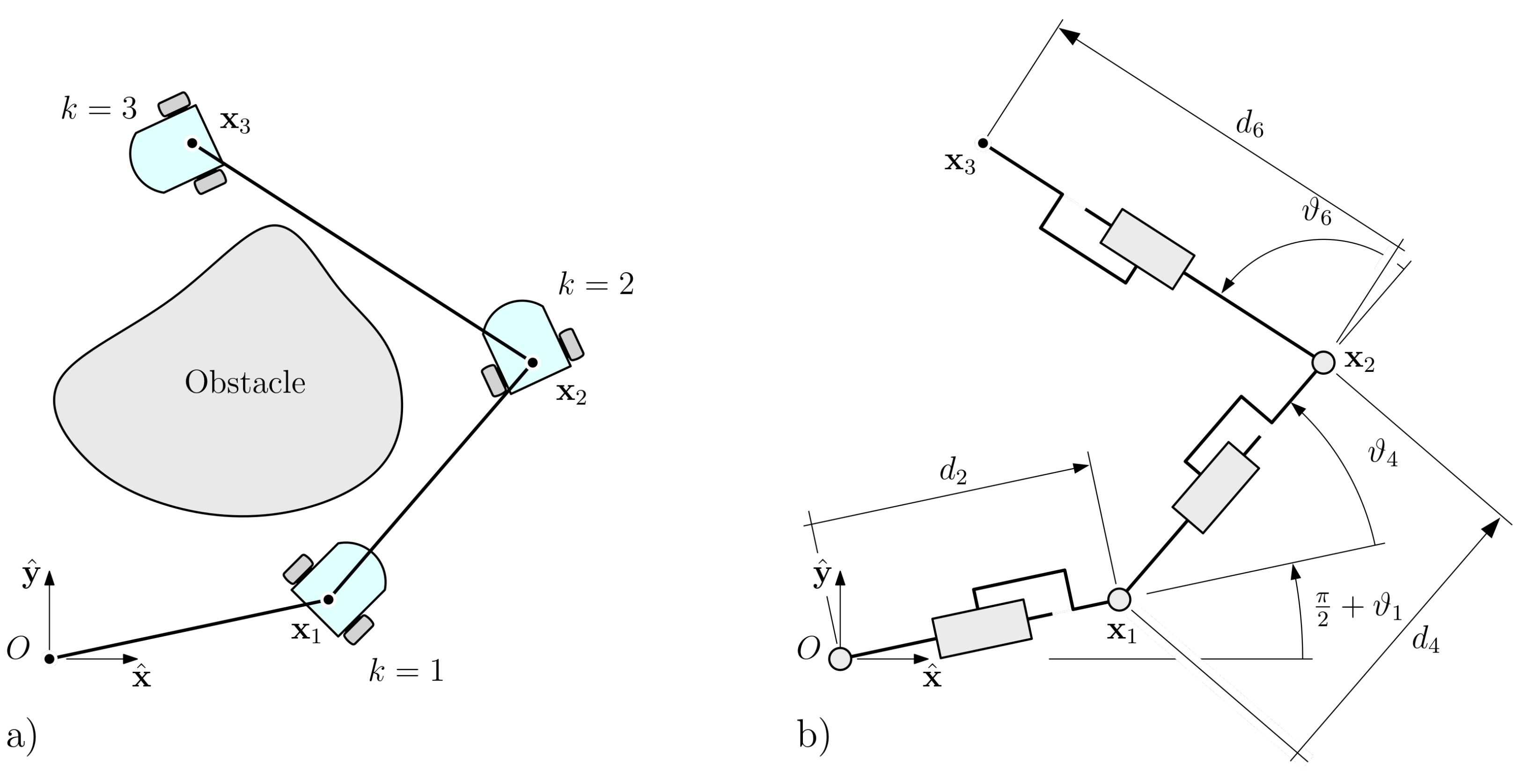
This section will present how the approach described in Section 3 has been used to solve a specific real problem. We consider three omnidirectional-drive mobile robots arranged on a flat surface cluttered by static obstacles; each robot is connected to the next by means of a tether which is not taut. We impose that the mobile robots have a safety radius of $0.5\mathrm{m}$. The first robot has a tether connecting it to the ground; the last robot has a tether connecting it only to the previous one. Each mobile robot is equipped with a winch that manages the tether by exerting a constant tension. The system can be seen in Figure 2a; while in Figure 2b the analogy to a planar RM is immediately apparent.

The objectives that we want to achieve in this problem are summarized in:

• The mobile robots must be moving simultaneously in a cluttered environment; the leader must be capable of reaching the target point in the task space by tracking a reference trajectory;
• The robots must not collide with themselves and with the obstacles;
• Neither of the three tethers must touch the ground nor hit any of the surrounding obstacles;
• The distance between each consecutive robot must be a trade-off between their local minimization and uniformity with the other tethers length.

Based on the schematics proposed in Figure 2b, the parameters relative to the D-H convention are reported in

Table 1. Denavit–Hartenberg parameters table for the robotic manipulator described in Figure 2a.

Link	a	d	$\mathit{\alpha }$	$\mathit{\theta }$
1	0	0	$\pi /2$	$\pi /2+{\vartheta }_1$
2	0	$d_2$	$-\pi /2$	0
3	0	0	$\pi /2$	${\vartheta }_3$
4	0	$d_4$	$-\pi /2$	0
5	0	0	$\pi /2$	${\vartheta }_5$
6	0	$d_6$	$-\pi /2$	0

.

A general task in the bi-dimensional space is completely defined if coordinates $(x,y)$ and orientation $\varphi$ of the end-effector are given relative to a fixed frame. If the task is about positioning the end-effector with no regard to its orientation, the functional redundancy can be exploited leading to $r=4$.

4.1. Tasks Definition

In order to achieve the objectives described above, some constraints to the system must be specified. As discussed in Section 3, this can be done by using the task priority framework, via the introduction of multiple suitable secondary tasks.

In this section, the primary task is illustrated, followed by the definition of the secondary tasks. The Jacobians defined in the following sections are substituted in Equations (5) and (6).

4.1.1. Primary Task: Trajectory Tracking

The primary task of the equivalent RM is referred to its end-effector tracking a reference trajectory. Using Equation (3), the primary task can be described by the following equation:

$${\dot{\mathit{x}}}_{\mathit{e}}={\mathit{J}}_{\mathit{e}}\left(\mathit{q}\right)\dot{\mathit{q}}$$

(8)

where ${\dot{\mathit{x}}}_{\mathit{e}}\in {\mathbb{R}}^2$ is the task velocity vector of the end-effector and ${\mathit{J}}_{\mathit{e}}\left(\mathit{q}\right)\in {\mathbb{R}}^{2\times 6}$ is the Jacobian associated with the end-effector, and it is computed as follows:

$${\mathit{J}}_{\mathit{e}}\left(\mathit{q}\right)=[J_1,J_2,\cdots ,J_6]$$

(9)

where, if we assume that ${\mathit{p}}_p^0$ and ${\mathit{p}}_k^0$ are respectively the position vector of a generic point ${\mathit{p}}_p$ and the position vector of the k-th joint, both with respect to the base frame,

$$J_k=\{\begin{array}{ccc}\Gamma ·{\Omega }_k·\Lambda \hfill & \hfill \mathrm{if}k-\mathrm{th}\mathrm{prismatic}& \hfill \left(10\right)\\ \Gamma ·\left[{\Omega }_k\times ({\mathit{p}}_{\mathit{p}}^{\mathbf{0}}-{\mathit{p}}_{\mathit{k}}^{\mathbf{0}})\right]·\Lambda \hfill & \hfill \mathrm{if}k-\mathrm{th}\mathrm{revolute}& \hfill \left(11\right)\end{array}$$

with

$${\Omega }_k={\displaystyle \prod _{i=1}^k}{T}_i^{i-1},\Lambda ={\left[\begin{array}{cccc}0& 0& 1& 0\end{array}\right]}^T,\Gamma ={\left[\begin{array}{cc}\Lambda & \Lambda \end{array}\right]}^T$$

(12)

If the Jacobian referred to the end-effector has to be computed, the position vector of the end-effector ${\mathit{p}}_e^0$ must be substituted in the generic position vector ${\mathit{p}}_p^0$.

4.1.2. Secondary Task: Joint Limits Avoidance

The first task with a lower priority than that of the primary task that will be introduced is the so-called joint limits avoidance. The GPM will be used, and the objective function can be constructed as follows: [40]:

$$w\left(\mathit{q}\right)=-\frac{1}{2n}\sum _{i=1}^n\frac{{(q_i-q_{i,t})}^2}{(q_{i,M}-q_{i,m})}$$

(13)

where $q_i$ is the i-th joint variable, while $q_{i,t}$, $q_{i,M}$ and $q_{i,m}$ are respectively the desired, the maximum and the minimum values of the i-th joint. In this case, there are no limitations on the revolute, while there are on the prismatic ones. More precisely, the minimum value for the prismatic joint is directly related to the dimensions of the robots, and it is defined as a function of the two consecutive robot’s safety bubbles; the maximum joint value is defined instead by solving the catenary problem, i.e., find the maximum distance between the robots such that the tether does not touch the ground.

By using Equation (7) and substituting constant gain $k_0$ with a diagonal gain matrix $\mathit{K}\in {\mathbb{R}}^{6\times 6}$, which will be used to give more importance to a specific joint variable with respect to the others, we obtain ${\dot{\mathit{q}}}_{\mathbf{0}}=\mathit{K}\widehat{\mathbf{\phi }}$, where $\widehat{\mathbf{\phi }}\in {\mathbb{R}}^6$ is a vector whose i-th component is defined as ${\widehat{\phi }}_i=(q_{i,t}-q_i),\forall i=1,\cdots ,n$. The values resulting from the differentiation of Equation (13) are grouped into the ${\mathit{K}}_{i,i}$ elements of the matrix diagonal. The coefficients ${\mathit{K}}_{i,i}=0$, for $i=1,3,5$, have been set this way because there are no limitations on the revolute joints, i.e., $q_i\in [-\pi ,\pi ]$, with $i=1,3,5$.

The Jacobian $\mathit{J}\left(\mathit{q}\right)\in {\mathbb{R}}^{2,6}$ associated with this task is the one associated with the end-effector defined in Equation (9).

4.1.3. Secondary Task: Obstacle Avoidance

In order to make the robots move into the task space safely, some control is needed in order for the robots to avoid colliding with objects. In addition, this can be obtained by exploiting some number of DORs and then defining a sub-task for the obstacle avoidance, as in the previous subsection.

Suppose that the end-effector is already following a free obstacle path; this sub-task allows for generating internal motions of the system in order to reconfigure the structure so that the inner links do not collide with obstacles.

As described in [28], in every time step, a critical point ${\mathit{x}}_{\mathit{c}}$ must be defined. This is defined as the the point along the manipulator that has a minimum distance from the obstacle. This task can be written in a differential form as:

$${\dot{\mathit{x}}}_{\mathit{c}}={\mathit{J}}_{\mathit{c}}\left(\mathit{q}\right)\dot{\mathit{q}}$$

(14)

where ${\dot{\mathit{x}}}_{\mathit{c}}\in {\mathbb{R}}^2$ is the evasion speed vector, and ${\mathit{J}}_{\mathit{c}}\left(\mathit{q}\right)\in {\mathbb{R}}^{2\times 6}$ is the Jacobian associated with the critical point. This point is located along the manipulator chain; as such, the associated Jacobian ${\mathit{J}}_{\mathit{c}}\left(\mathit{q}\right)$ depends on the relevant link corresponding to this location, as follows:

$$J_c=\left\{\begin{array}{cc}\left[\begin{array}{cccccc}{J}_1& 0& 0& 0& 0& 0\end{array}\right]\hfill & {\mathit{x}}_{\mathit{c}}\in {\mathrm{Link}}_1\hfill \\ \left[\begin{array}{cccccc}{J}_1& J_2& J_3& 0& 0& 0\end{array}\right]\hfill & {\mathit{x}}_{\mathit{c}}\in {\mathrm{Link}}_2\hfill \\ \left[\begin{array}{cccccc}{J}_1& J_2& J_3& J_4& J_5& 0\end{array}\right]\hfill & {\mathit{x}}_{\mathit{c}}\in {\mathrm{Link}}_3\hfill \end{array}\right.$$

(15)

where $J_k$ is computed using Equations (10) and (11), and the position vector ${\mathit{x}}_{\mathit{c}}$ must be substituted in place of ${\mathit{p}}_{\mathit{p}}^{\mathbf{0}}$.

The evasion speed ${\dot{\mathit{x}}}_{\mathit{c}}$ is a vector pointing in the direction that maximizes the distance between the critical point and the closest obstacle. This consideration leads to a definition of scalar objective function, which has to be maximized:

$$w\left(\mathit{q}\right)=\left|\right|{\mathit{d}}_{\mathit{c}}-{\mathit{x}}_{\mathit{c}}\left|\right|$$

(16)

where ${\mathit{d}}_{\mathit{c}}$ is the position vector of the closest obstacle. For the definition of this sub-task in this paper, we will not directly use this function, rather, we will use its normalized gradient; we will define a nominal evasion speed and an activation function, as described in the following:

$$\left\{\begin{array}{cc}{\dot{\mathit{x}}}_{\mathit{c}}=v_0{\displaystyle \frac{\nabla w\left(\mathit{q}\right)}{\left|\right|\nabla w\left(\mathit{q}\right)\left|\right|}}\hfill & \left|\right|{\mathit{d}}_{\mathit{c}}-{\mathit{x}}_{\mathit{c}}\left|\right|<d_{min}\hfill \\ \\ {\dot{\mathit{x}}}_{\mathit{c}}=\mathbf{0}\hfill & \left|\right|{\mathit{d}}_{\mathit{c}}-{\mathit{x}}_{\mathit{c}}\left|\right|\ge d_{min}+\epsilon \hfill \end{array}\right.$$

(17)

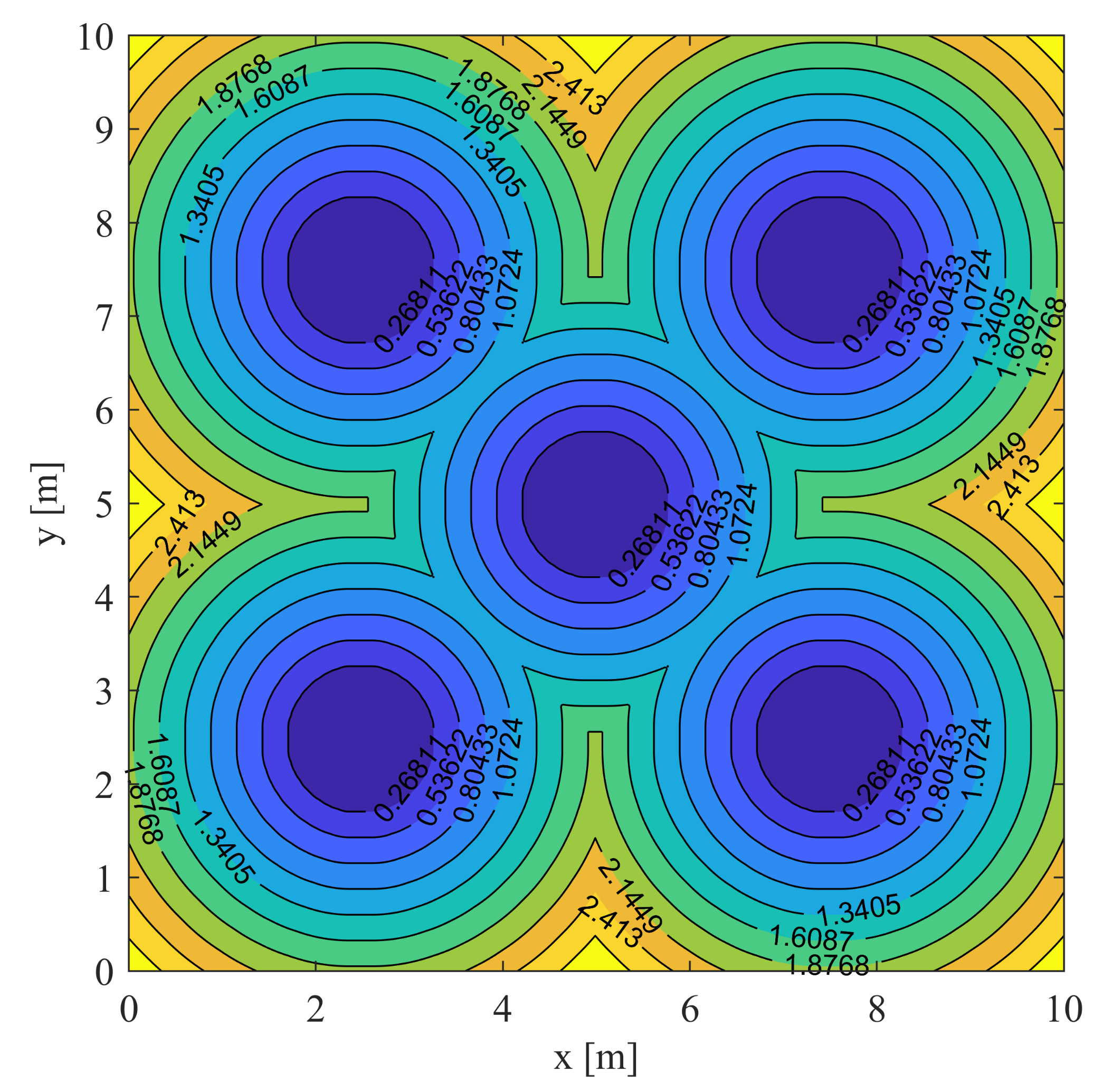
where $d_{min}$ is a specified safety distance which will trigger the activation of the sub-task. Note that $\epsilon >0$ has been introduced in order to avoid or at least reduce the Zeno Phenomenon; this will make the controller more stable and reduce the oscillations of the system. The scalar objective function $w\left(\mathit{q}\right)$ has been created in MATLAB over a discrete bi-dimensional grid, which has been constructed over the given map representing the working environment; to each grid cell, a value has been assigned representing the minimum Euclidean distance from the current cell and the closest cell containing an obstacle. If a cell contains an obstacle, the assigned distance value is set to zero. Subsequently, over the same grid, the gradient has been evaluated and mapped for future needs. As can be easily seen from Figure 3, the gradient direction is orthogonal to the level surfaces.

Two aspects are important about the definition of $w\left(\mathit{q}\right)$ (see Equation (16)): the first is that, with its mapping over a discrete grid, it is possible to represent any kind of obstacle, i.e., no restriction on convex and regular shapes. The second is that an integration with real range sensor data are trivial, e.g., ultrasonic, LiDAR or any point cloud based system.

Note that, while the evasion speed $v_0$ can be assumed constant, in order to achieve a smoother behavior, the speed $v_0=\raisebox{1ex}{$k_{v_0}$}\!\left/ \!\raisebox{-1ex}{$\left|\right|{\mathit{d}}_{\mathit{c}}-{\mathit{x}}_{\mathit{c}}\left|\right|$}\right.$ has been defined explicitly as inversely proportional to the critical distance ${\mathit{d}}_{\mathit{c}}$. Hence, a different Jacobian can be computed as follows:

$${\mathit{J}}_{\mathit{n}}\left(\mathit{q}\right)={{\mathit{n}}_{\mathit{c}}}^T{\mathit{J}}_{\mathit{c}}\left(\mathit{q}\right)$$

(18)

where ${\mathit{n}}_{\mathit{c}}=\raisebox{1ex}{$\nabla w\left(\mathit{q}\right)$}\!\left/ \!\raisebox{-1ex}{$\left|\right|\nabla w\left(\mathit{q}\right)\left|\right|$}\right.$ and ${\mathit{J}}_{\mathit{n}}\left(\mathit{q}\right)\in {\mathbb{R}}^{1\times 6}$ is the new Jacobian associated with the obstacle avoidance sub-task.

4.2. Control

In this subsection, the control architecture that will be used to achieve the requirements listed in the introduction of this section will be explained, and the relative control flow will be reported. The control is based on the CLIK (Closed Loop Inverse Kinematics) algorithm for the serial manipulators proposed in [23]. First, the end-effector tracking error vector needs to be defined at a given time t as follows:

$$\mathit{e}\left(t\right)={\mathit{x}}_{\mathit{d}}\left(t\right)-{\mathit{x}}_{\mathit{e}}\left(t\right)$$

(19)

where ${\mathit{x}}_{\mathit{d}}\left(t\right)$ is the position vector of a point along the trajectory and ${\mathit{x}}_{\mathit{e}}\left(t\right)$ is the position vector of the end-effector both at time t. By differentiating Equation (19) and by using Equation (3), we obtain $\dot{\mathit{e}}\left(t\right)={\dot{\mathit{x}}}_{\mathit{d}}\left(t\right)-{\mathit{J}}_{\mathit{e}}\left(\mathit{q}\right)\dot{\mathit{q}}$. We choose the equivalent linear system $\dot{\mathit{e}}\left(t\right)+\mathit{Ke}\left(t\right)=0$ which has been demonstrated to be asymptotically stable for a positive-defined gain matrix $\mathit{K}$; this leads to the algorithmic solution for the IK for trajectory tracking of the end-effector:

$$\dot{\mathit{q}}={\mathit{J}}_{\mathit{e}}^{\#}\left(\mathit{q}\right)({\dot{\mathit{x}}}_{\mathit{d}}\left(t\right)+\mathit{Ke}\left(t\right))$$

(20)

Since the trajectory tracking is defined as the primary task, then Equation (20) can be substituted in Equation (5). Substituting the sub-tasks defined in the previous section as well, we obtain the algorithmic solution for the multi-task RM. Time-integration provides the joints variable vector $\mathit{q}$. Based on Equation (5), we then obtain:

$$\mathit{q}\left(t\right)={\int }_{t_0}^t{\mathit{J}}_{\mathit{e}}^{\#}\left(\mathit{q}\right)({\dot{\mathit{x}}}_{\mathit{d}}+\mathit{Ke})dt+{\int }_{t_0}^t\left(\sum _{i=2}^t{\mathit{P}}_{\mathit{i}-\mathbf{1}}^{\mathit{A}}\left(\mathit{q}\right){{\mathit{J}}_{\mathit{i}}}^{\#}\left(\mathit{q}\right){\dot{\mathit{x}}}_{\mathit{i}}\right)dt$$

(21)

where t is the number of secondary tasks. Since the integration has to be done numerically, Equation (21) must be discretized, the integrals must be substituted with a sum, and a proper sampling period has to be chosen.

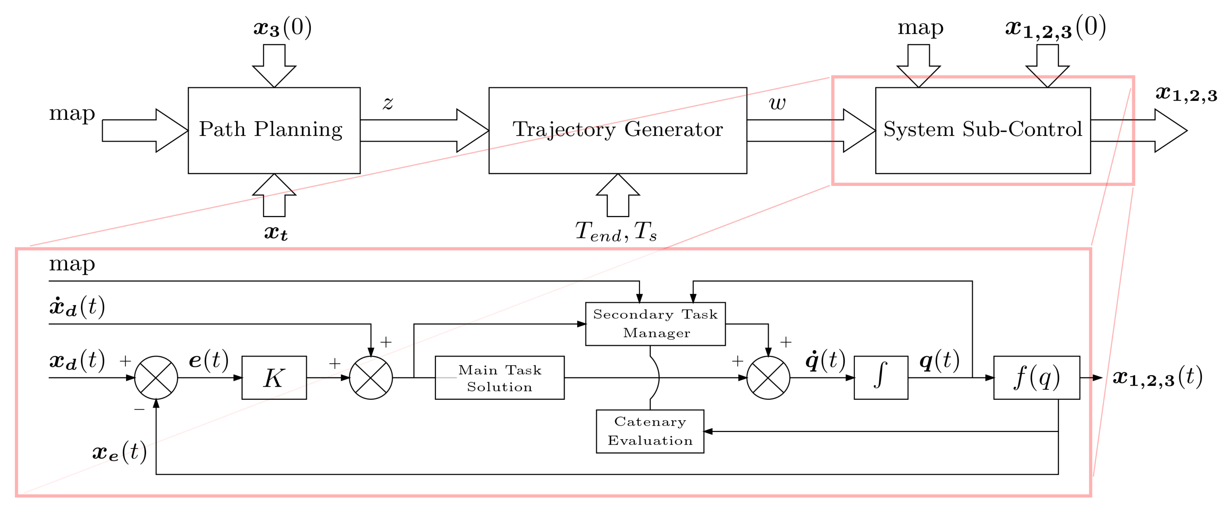
The control is of type “Centralized Control”. The control architecture can be split into three different main blocks, visible in Figure 4, and briefly described below:

• Planner: Is responsible for generating a free obstacle path for the end-effector of the equivalent RM starting from an already known discrete map of the environment, and the initial pose of the equivalent RM. The free obstacle path is obtained by means of a graph search algorithm, more precisely the RRT* [41], and stored in a data structure we will denote with $\mathit{z}$.
• Trajectory Generator: Given a desired time, it is responsible for generating a trajectory passing through the points generated by the planner block. To generate a time based trajectory, a B-spline has been used. The duration of the trajectory has been fixed to $T_{end}=15$ s and the sampling period to $T_s=0.05$ s. In particular, by denoting as w the trajectory data structure, composed by $N=T_{end}/T_s$ points, we have $\mathit{w}=[\mathit{X},\dot{\mathit{X}},\ddot{\mathit{X}}]=f(T_{end},T_s,\mathit{z})$ with its components the time-series of values $x\left(t\right)$, $\dot{x}\left(t\right)$ and $\ddot{x}\left(t\right)$ respectively, for $t=0,\cdots ,T_{end}$.
• System Sub-Control: This is the most important block because it is here that the CLIK algorithm works. It takes as input the trajectory data structure w generated from the Trajectory Generator and an additional data structure containing important data about the map (such as the distance field and its gradient). As output, this block returns a data structure containing the three trajectories the TMRs have to track, denoted with $x_{1,2,3}$ in Figure 4. By expanding this block, a subsystem control loop can be found, which is composed by three main parts:

  (a)

  Main CLIK Algorithm: It gives a reference signal to the RM’s end-effector, which has to track it, and computes its IK;

  (b)

  Secondary Tasks Manager: it computes and arranges the terms used in the multi-task framework;

  (c)

  Parallel Catenary Evaluation: it checks at each iteration the actual pose and how the catenary is mapped. It re-arranges the gain matrix of the joints limits avoidance sub-task in order to regulate the elongation of the tether.

The Secondary Task Manager is a Finite State Automaton with the two following distinct states:

• If all the links of the equivalent manipulator are out of the danger collision area, only the primary task and the joints limit avoidance are activated.
• If some point of any link enters inside the danger area, then the sub task of obstacle avoidance activates, taking the priority of the joints limits avoidance, while the latter priority is been lowered. This has the effect of sacrificing part of the minimization of the distance between each mobile robots, but gaining more flexibility to avoid obstacles. This state remains active until all points are outside of the danger zone.

At each iteration, Equation (2) is used to map the robot positions from the equivalent RM joint variables and then stored, generating then three different trajectories each robot has to follow; this can be seen in the main loop in Figure 4.

4.2.1. Parallel Catenary Evaluation

Since the tethers are modeled as prismatic joints to threat this multi robotic system kinematically as one single robot, the real behavior of tethers must be computed and characterized in parallel with the control of the RM. This, in particular, is done to prevent the cable from touching the ground.

Flexible tethers can be modeled with splines, catenaries and parabolas [42]. The catenary is a function of the height of the suspending points and of the cable tension and weight. Its parametric equation [43] is presented as follows:

$$y=c\left(cosh\left(\frac{x}{c}\right)-1\right)$$

(22)

where $c=\raisebox{1ex}{$T_0$}\!\left/ \!\raisebox{-1ex}{$\rho g$}\right.$ and $T_0$, $\rho$ and g are respectively the horizontal tension of the cable, its specific weight and the gravitational acceleration. The pair $(x,y)$ is the coordinate system used for the parameterization that is centered at the minimum point of the curve. Considering the height of the robots $H=0.43\mathrm{m}$, a pulley resisting torque $T_r=1.35\mathrm{N}\mathrm{m}$ and radius $r=0.1\mathrm{m}$. By using Equation (22), a cable specific weight $\rho =0.15\mathrm{k}\mathrm{g}/\mathrm{m}$, it follows that the maximum allowed horizontal distance between the robots, which guarantees that the cable does not touch the ground, is $d_{max}=5.84\mathrm{m}$.

Based on the equations reported in Equation (22) for each value of the sag—or equivalently the robot horizontal distance—a value for the joints limits avoidance gain $\mathit{K}$ must be specified. To achieve this, an appropriate function has been defined and composed by a sum of two exponential functions and a constant gain G, as follows:

$${\mathit{K}}_{i,i}\left(q_i\right)=a_1{e}^{b_1{q}_i}+a_2{e}^{b_2{q}_i}+G,i=2,4,6$$

(23)

which takes as input the robot horizontal separation. The exponential functions have the aim of gradually increasing the gains used in the joints limits’ avoidance secondary task in specific conditions. This happens if either the robots’ horizontal separation approaches the safety minimum distance, which assures that they do not collide, or the maximum distance $d_{max}$ as the distance at which the cable touches the ground.

4.2.2. Parameters Tuning, Performance Function Definition and Optimization

To achieve a global smooth behavior and minimum energy loss, many parameters of the system must be tuned, e.g., the gains and the evasion speed. For this reason, it is necessary to define performance functions in order to compare single simulations. To provide coherent samples, the environment map shall be the same for all simulations.

The performance functions that have been taken into consideration are reported in the following: the values are discretized in N samples indexed as $k=0,\dots ,N$.

These have to be simultaneously minimized:

$$\begin{array}{cc}\hfill f_1& =\sum _{k=0}^N\dot{\mathit{q}}\left(k{T}_s\right){}^{\mathit{T}}\dot{\mathit{q}}\left(k{T}_s\right)\hfill \end{array}$$

(24)

$$\begin{array}{cc}\hfill f_2& =\sum _{k=0}^N\left[{(d_1-d_2)}^2+{(d_2-d_3)}^2+{(d_3-d_1)}^2\right]\hfill \end{array}$$

(25)

$$\begin{array}{cc}\hfill f_3& =\sum _{k=1}^N|\left|{\mathit{x}}_{\mathit{e}}\left(k{T}_s\right)\right)-{\mathit{x}}_{\mathit{d}}\left(k{T}_s\right){\left|\right|}^2\hfill \end{array}$$

(26)

$$\begin{array}{cc}\hfill f_4& =\sum _{k=1}^N\stackrel{⃛}{\mathit{q}}{\left(k{T}_s\right)}^T\stackrel{⃛}{\mathit{q}}\left(k{T}_s\right)\hfill \end{array}$$

(27)

Note that Equation (24) represents the energy spent by the hypothetical motors of the serial equivalent manipulator. Equation (25), where $d_i=f\left(k{T}_s\right)$ with $i=1,\cdots ,3$ is the discrete equivalent of $q_{2i}$ (the $2i$-th prismatic joint elongation), takes into account the uniformity of the distance between the robots. By minimizing this function, we aim at keeping the robot separation distance constant. Equation (26) quantifies how accurate the manipulator end-effector is when tracking a reference trajectory. Finally, Equation (27) quantifies the jerk of the structure during the whole motion, whose minimization leads to a smoother motion of the structure.

If the robot manipulator end-effector is unable to terminate the simulation for any reason, a blind penalty is applied, thus having $f_i=+\infty$. Failures of this type occur when large values lead to system instability, the links of the robot colliding with obstacles or the minimum distance between robots exceeds the maximum allowed.

For the optimization, a genetic algorithm has been used for the multi objective optimization process (MOGA) and, in the end, a proper set of parameters has been chosen.

5. Results

After the tuning of parameters, simulations over three different scenarios have been conducted; more precisely:

-

Scenario A; a square room in which five obstacles are present, represented by disks with a certain diameter; the objective is for the last mobile robot to position itself behind the obstacle placed in the middle of the room;

-

Scenario B; an environment in which there is a high-curvature path representing a curved corridor leading out of the room. The aim in this scenario for the last robot is to reach the end of the corridor.

-

Scenario C; a square room in which some walls are modeled in order to simulate a small maze. The aim in this scenario is for the last robot to position itself in the top right corner of the room;

-

Scenario D; a square room where a model of the Cessna C-172 is present, which needs to be worked on by the robots, for example, in this case robotic painting. The aim in this scenario is for the last robot to move around the plane and position on the opposite side.

In order to take into account the physical dimensions of the robots, the obstacles are grown in size accordingly.

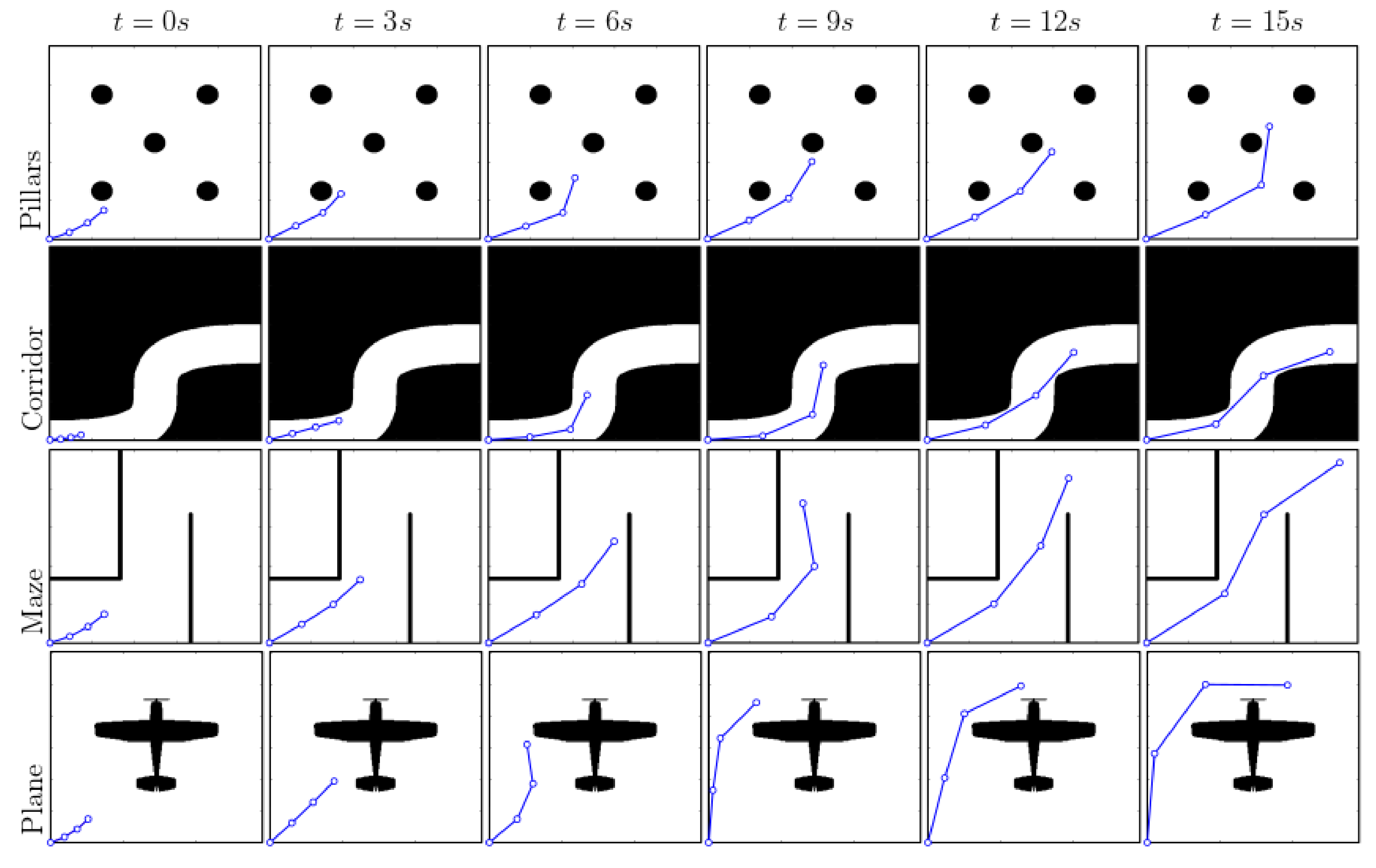
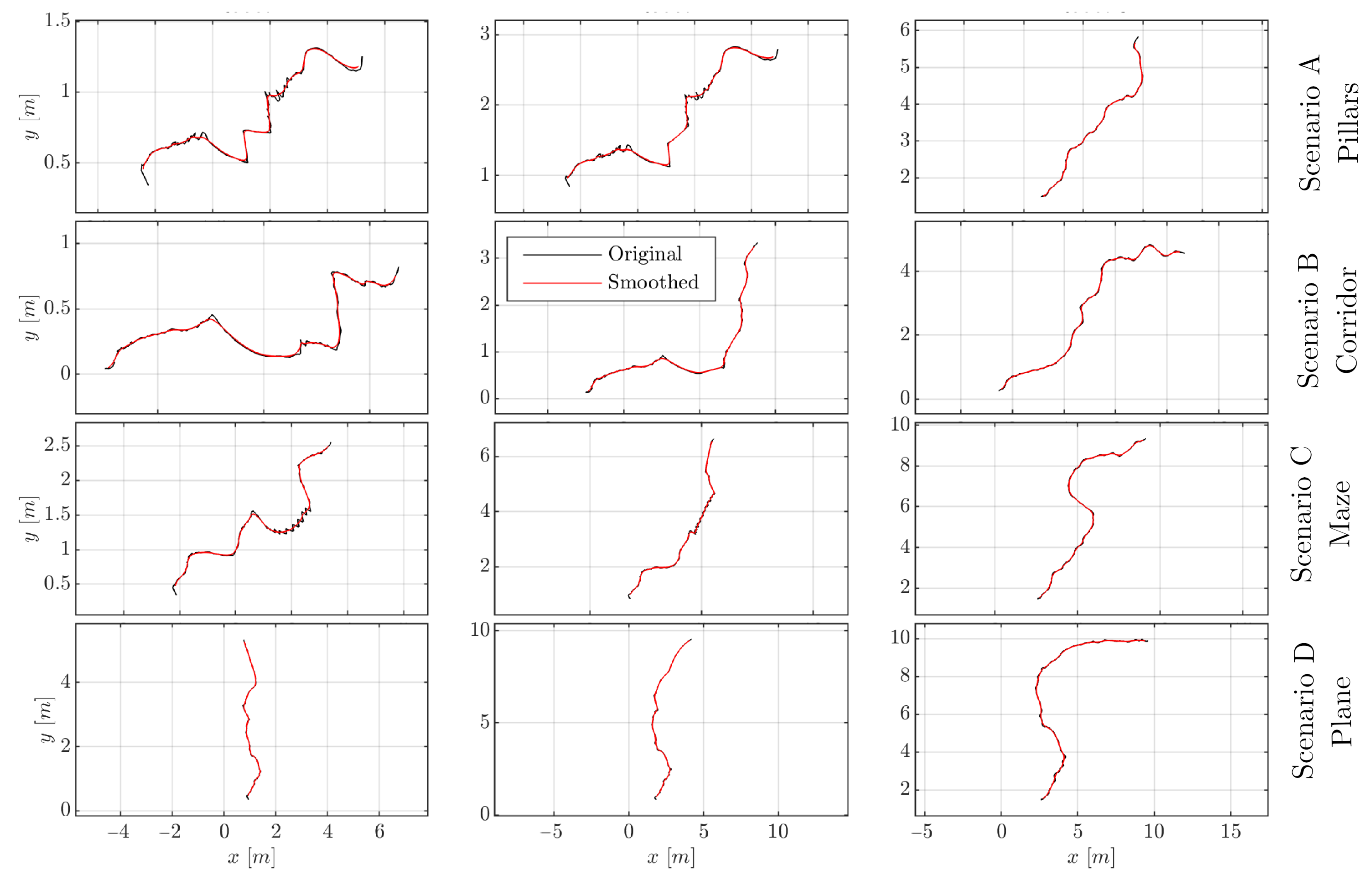
In Figure 5, some runs are reported of the equivalent manipulator pose. The pose is evaluated over a fixed time step of three seconds for all four of the different scenarios. The straight lines represent the tether as viewed from the top or, equivalently, the links of the manipulator; in other words, the ends of the lines represent either the mobile robots or the manipulator revolute joints. It can be clearly seen that, near the obstacles, the system re-configures its structure in order to avoid them; at the same time, it tries both to minimize the horizontal separation distances between consecutive mobile robots and to keep them as close as possible to each other. Finally, it can be said that neither the mobile robots nor the tethers touch the obstacles during the whole simulation. Figure 6 shows the generated trajectories that each of the mobile robots has to follow for each scenario: in the top row for the scenario A; in the second row for the scenario B, in the third row for the scenario C and in the bottom row for the scenario D. With the exception of the trajectories of the end-effector (Robot 3), which have been pre-computed at the planner level, all other trajectories show spikes due to both numerical oscillations and the sudden activation/deactivation of the sub-tasks. In order to remove the spikes, the trajectories have been smoothed by filtering. The results of this process are the trajectories shown in red.

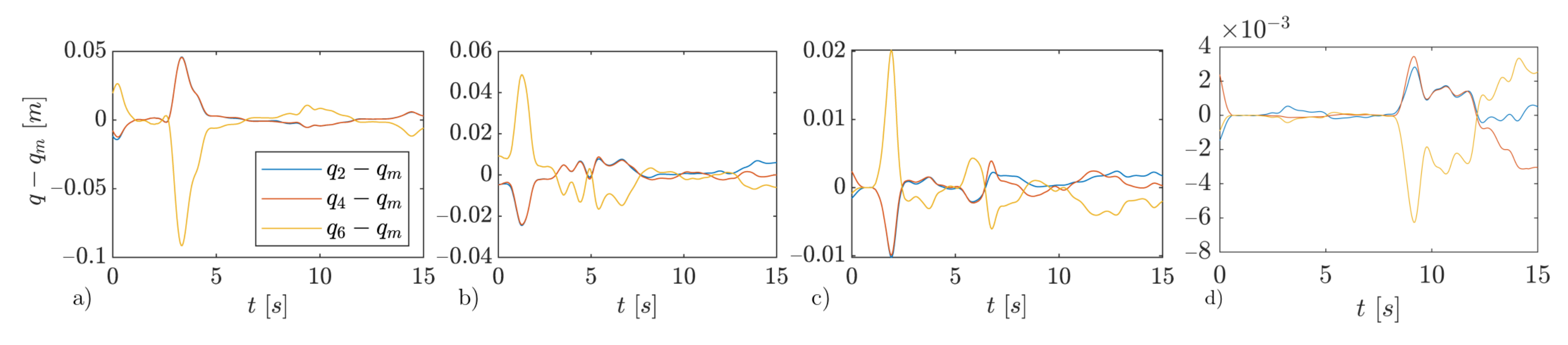
Recall that $q_2$, $q_4$ and $q_6$ in the equivalent manipulator represent both the prismatic joints elongation and the horizontal separation between two consecutive mobile robots. Figure 7 shows the evolution over time of three distance errors. These are are defined as the difference between the horizontal separation of the mobile robots and the mean of all of them at a given time. During the simulation, the errors stay close to zero except at certain times; this is due to the fact that, at that time, the structure is trying to avoid obstacles by activating the obstacle avoidance secondary task and lowering the priority of the joints limits avoidance one. This leads to an increase of tracking errors. For scenarios B and C, this error remains within 0.05 m; for the scenario C, instead, it is less than 0.10 m; and, finally, for scenario D, it is less than $0.008$ $\mathrm{m}$ in absolute value.

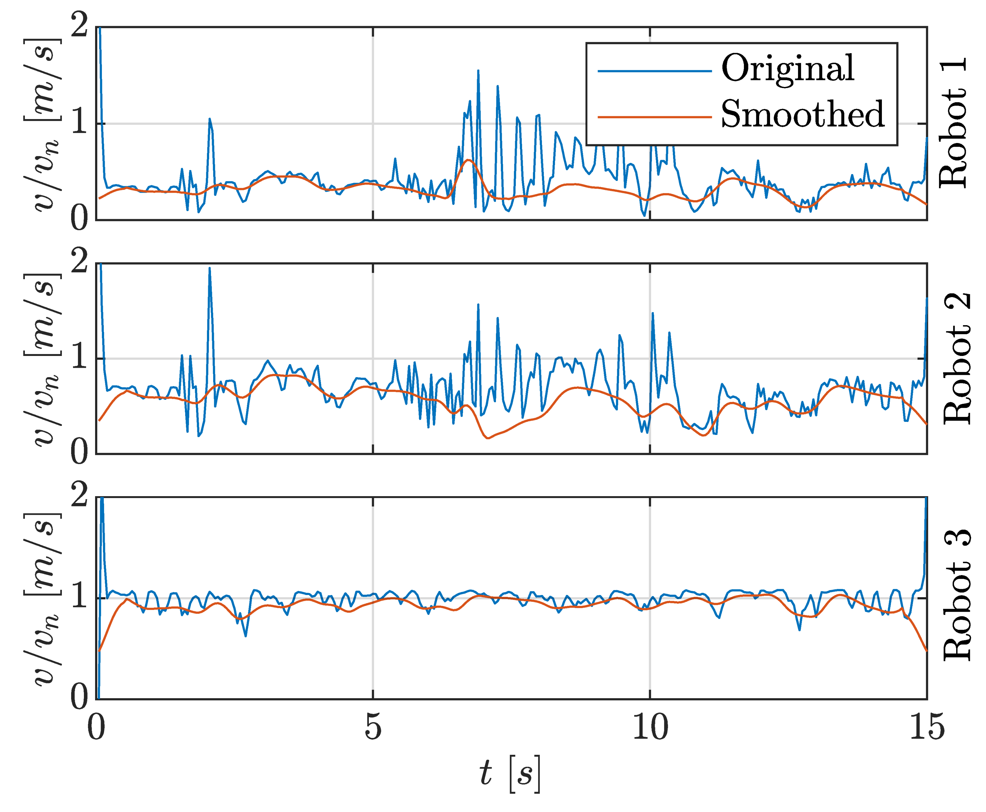
Figure 8 contains information about the instantaneous speed that each mobile robot must have in order to complete the three generated trajectories. The three speed distributions refer to the trajectories generated for the scenario B. The speed is expressed as normalized speed. The normalization has been done with respect to the nominal speed $v_n$ defined as the mean speed the end-effector (Robot 3) must have in order to track the entire trajectory in the given simulation time. The effects of the filtering can be seen clearly in this figure as well; in the original trajectories, the spikes have the effect of producing high instantaneous speeds and accelerations. By filtering the original trajectories, we can obtain a better distribution of the speed each mobile robot must have in order to follow its reference trajectory; this speed distribution is expressed by the red curve.

5.1. Fitness: Sensitivity Analysis

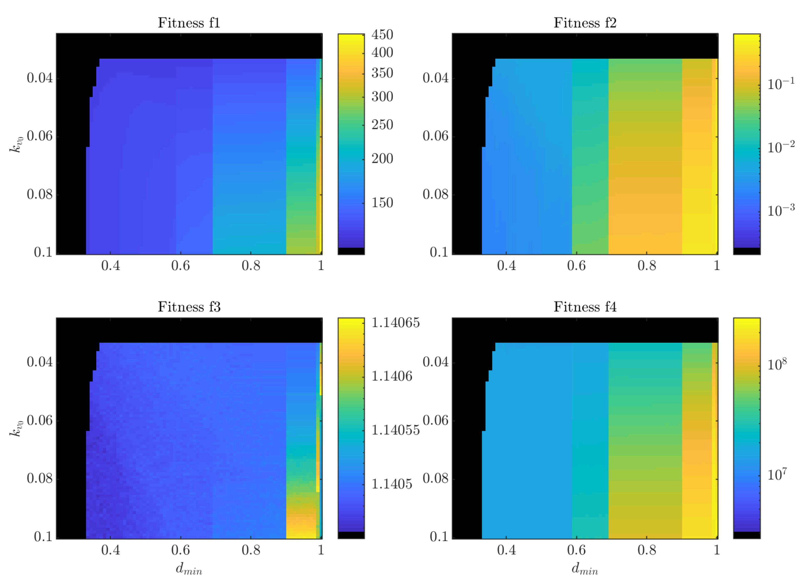
In order to grasp the mechanisms behind variations in the fitness functions presented in Equations (24)–(27), we present a sensitivity analysis on two specific parameters: the constant of evasion speed $k_{v_0}$ and the minimum distance $d_{min}$ that activates the obstacle avoidance secondary task. The selection was made based on the observation that these are the two most influential parameters that are also based on physical quantities; indeed, most other parameters are related to the gains of the controller, and, as such, do not capture the high-level behaviour of the robot well. The interval of variation of the chosen parameters is defined as $k_{v_0}=k_{v_0}^{*}+[-50\%,+100\%]$, and $d_{min}=d_{min}^{*}+[-50\%,+100\%]$, where $k_{v_0}^{*}=0.05{\mathrm{m}}^2/\mathrm{s}$, and $d_{min}^{*}=0.5\mathrm{m}$. The fitness functions show values in the following intervals: $f_1\in [123.9412,453.7501]\mathrm{J}$, $f_2\in [0.0021,0.6446]{\mathrm{m}}^2$, $f_3\in [1.1405,1.1407]{\mathrm{m}}^2$ and $f_4\in [0.1559\times {10}^8,2.7352\times {10}^8]\mathrm{m}/{\mathrm{s}}^3$. The results of this analysis are reported in Figure 9, for each of the fitness functions described in Section 3. The plots show several aspects that are discussed in the following.

In general, the fitness $f_2$ remains very small in every configuration $(k_{v_0},d_{min})$, which stands to show that the approach is effective in keeping the separation distance uniform between the robots. This is mostly true also for $f_3$, which shows that the tracking error of the robots is kept at a low level for a vast majority of the configurations $(k_{v_0},d_{min})$.

The area colored in black represents configurations of the parameters $k_{v_0}$ and $d_{min}$ that lead to an unfeasible path-planning, i.e., one where the robot collides with the obstacles. Vertical bands are noticeable throughout the response surfaces of the fitness functions; these appear aligned between the various plots, and show a degree of uniformity between values of $d_{min}$; in other words, it seems that $d_{min}$ influences the performance of the system in a step-like manner. This is not true in the case of $k_{v_0}$, which indeed shows a very gradual influence.

These large discontinuities are caused by the activation of the obstacle avoidance secondary task, which introduces large penalties to the overall performance of the system. In fact, while the main task works under the criterion of a minimal energy approach (see the first term of Equation (4) which implicitly introduces this behavior), the secondary tasks completely disregard this constraint, thus causing large losses in fitness upon activation. Geometrically, during obstacle avoidance, the algorithm generates sudden evasive motions roughly orthogonal to the general direction of travel, which negatively affects the fitness related to energy. Thus, as expected, this is very apparent in the case of $f_1$ and $f_4$, i.e., energy and jerk.

The fact that the contribution of $d_{min}$ on $f_i$ is larger than that of $k_{v_0}$ is likely because the former has a direct influence on the activation of the obstacle avoidance task, i.e., when it activates, while the latter only influences how this specific task behaves.

Given the topology of the response surfaces of all fitness functions, it is apparent that the task of finding an optimal configuration $(k_{v_0},d_{min})$ is that of choosing both low values of $k_{v_0}$ and of $d_{min}$. However, it should be noted that this goes in the direction of the unfeasible configurations (shown in black in the plots). As such, if we consider this a multi-objective optimization problem, the border between the black area and the colored area can be identified as the Pareto front of the problem; as such, configurations in this location have optimal values but—being so close to the unfeasible region—minimal robustness.

5.2. ROS and Gazebo Simulation

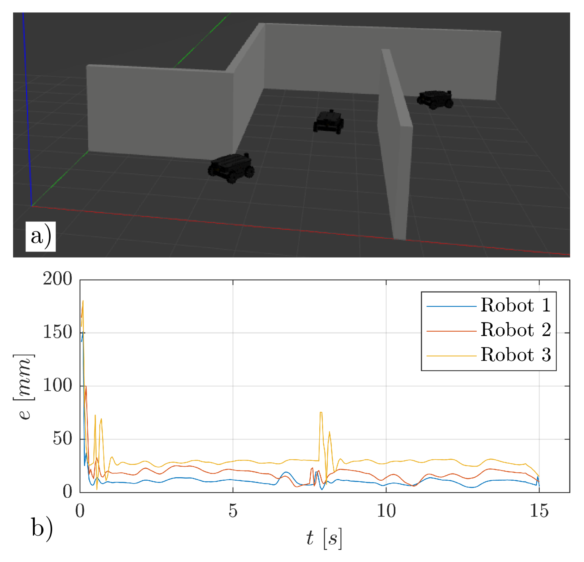
In order to prove the effectiveness and soundness of the methodology presented in the previous section, two simulations are performed on Gazebo, respectively for the case of the scenarios C and D. Gazebo is a kinematics and dynamics simulator of robotic systems based on the Robot Operating System (ROS) framework.

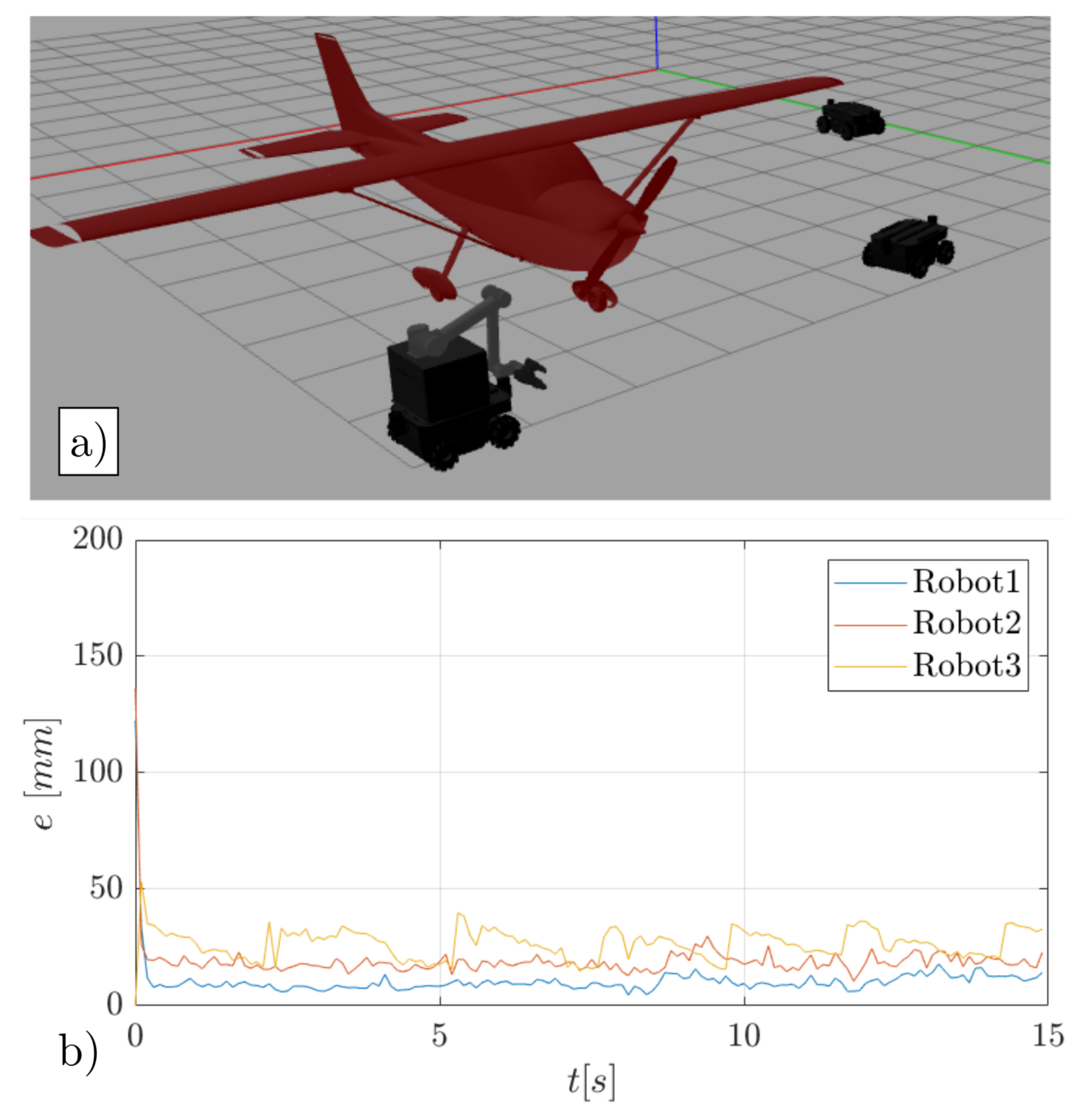
In order to run a multi-robot simulation, two ROS packages have been written in Python and XML languages, which contribute to the overall simulation. The first package is responsible for starting the simulation environment, based on the map used in the other simulations, and spawning three different mobile robots in the Gazebo simulator. The selected robots are three Neobotix MPO-500 for the case of the scenario C; and two MPO-500 and a MMO-500 for the case of scenario D. They are all ROS enabled omni-directional drive mobile robots, but, differently from the other platforms, the MMO-500 one mounts a UR10 robotic arm on it. The other package is responsible for starting as many ROS nodes as the number of mobile robots present in the environment, and connecting with them. Each of these nodes represents a single process, responsible for loading the json file containing the previously generated smoothed trajectories and assigning the correct one to the robot; moreover, it runs a general PID regulator for trajectory tracking and has a routine that stores the robot state variables into another json file for post processing purposes. It should be noted that each robot has its own controller, both for coherence to the real-world scenario, and since it has the benefit of reducing the computational load. In Figure 10a, an image is reported representing the final instant of the simulation conducted in scenario C. Figure 10b instead shows three curves, one for each mobile robot, which represents the tracking error. Figure 11, instead, illustrates the same results, this time for case D.

During the simulations, none of the robots collided with each other or the walls, always keeping a safety distance.

6. Conclusions

By using the kinematic analogy between a chain of TMRs and an open-chained serial robotic manipulator, and by exploiting its redundant degrees of freedom, it has been possible to generate and plan the trajectories for each of the mobile robots subjected to constraints. Constraints in this case are: avoiding obstacles, keeping the robots at a safe distance, keeping the distance between adjacent robots less than the maximum admissible by the catenary; minimizing the distance between them; keeping this distance uniform between the robots. The methodology shows limited irregular motion at times; for example, when the obstacle avoidance secondary task activates in order to avoid a close obstacle, it sometimes produces a sudden lateral motion. It is important to remark that, in this paper, the mobile robots’ motion capabilities have been considered omnidirectional; this grants feasible lateral movements over the trajectories, which is an advantage. On the other hand, more care should be taken if the mobile robots are not omnidirectional, e.g., differential drive robots. In that case, it could lead to an increase of the tracking error on the nominal trajectories for those robots. A solution could be to grow the obstacles, in order to take into account not only the physical dimensions of the robots but also the turning radius.

Furthermore, results show that the solution is subject to numerical oscillations, which can be minimized with some post-processing on the trajectories. We believe that these oscillations could be reduced, as is done in other works [28,44,45], by granting a smooth transition between the tasks, for example with a blending function instead of the current sudden transition. Moreover, from the sensitivity analysis, we have seen that the $d_{min}$ parameter, and, in general, the obstacle avoidance task, has a great influence on the fitness functions, thus reducing the robots’ performances, which can be seen from the functions related to energy and jerk. The same shows that the optimal behaviour of the overall system is achievable with configurations of the chosen parameters close to the failure configuration areas.

In future work, this strategy will be implemented on three real mobile platforms. The specific kinematics of these will be taken into account, moving away from the simple omnidirectional description given in this paper. One possible approach if the robots are omnidirectional will be to model the kinematic constraints as noise in the control algorithm to account for their dynamics. For other more limited kinematics (e.g., differential driven robots), more in-depth approaches will be studied. Moreover, the strategy and the code will be adapted and optimized for an online programming of the mobile robots. Future work also foresees the implementation of the approach with a higher degree of complexity; for example, three-dimensional scenarios will be considered. Moreover, we will investigate the method in cluttered and basically unknown environments, or in a dynamic one. Finally, we believe that, instead of a passive tether, it would be useful to introduce an active system that controls the torque of the pulleys in order to increase or decrease the tension acting on the cable. This could be useful in rearranging the shape of tether, e.g., to overcome low height obstacles.

References

- Ajwad, S.; Iqbal, J. Recent Advances and Applications of Tethered Robotic Systems. Sci. Int. 2014, 26, 2045–2051. [Google Scholar]
- Zhang, X.; Pham, Q.C. Planning coordinated motions for tethered planar mobile robots. Robot. Auton. Syst. 2019, 118, 189–203. [Google Scholar] [CrossRef] [Green Version]
- Fagiano, L. Systems of Tethered Multicopters: Modeling and Control Design. IFAC-PapersOnLine 2017, 50, 4610–4615. [Google Scholar] [CrossRef]
- Tognon, M.; Franchi, A. Nonlinear observer for the control of bi-tethered multi aerial robots. In Proceedings of the 2015 IEEE/RSJ International Conference on Intelligent Robots and Systems (IROS), Hamburg, Germany, 28 September–2 October 2015; pp. 1852–1857. [Google Scholar]
- Kosarnovsky, B.; Arogeti, S. A String of Tethered Drones—System Dynamics and Control. In Proceedings of the 2019 European Conference on Mobile Robots (ECMR), Prague, Czech Republic, 4–6 September 2019; pp. 1–6. [Google Scholar]
- McLain, T.W.; Rock, S.M. Experimental Measurement of ROV Tether Tension. In Proceedings of the Intervention/ROV ’92, San Diego, CA, USA, 10–12 June 1992; pp. 291–296. [Google Scholar]
- McGarey, P.; Polzin, M.; Barfoot, T.D. Falling in line: Visual route following on extreme terrain for a tethered mobile robot. In Proceedings of the 2017 IEEE International Conference on Robotics and Automation (ICRA), Singapore, 29 May–3 June 2017; pp. 2027–2034. [Google Scholar]
- Krishna, M.; Bares, J.; Mutschler, E. Tethering system design for Dante II. In Proceedings of the International Conference on Robotics and Automation, Albuquerque, NM, USA, 25 April 1997; Volume 2, pp. 1100–1105. [Google Scholar]
- Nagatani, K.; Tatano, S.; Ikeda, K.; Watanabe, A.; Kuri, M. Design and development of a tethered mobile robot to traverse on steep slope based on an analysis of its slippage and turnover. In Proceedings of the 2017 IEEE/RSJ International Conference on Intelligent Robots and Systems (IROS), Vancouver, BC, Canada, 24–28 September 2017; pp. 2637–2642. [Google Scholar]
- Sebok, M.A.; Tanner, H.G. On the Hybrid Kinematics of Tethered Mobile Robots. In Proceedings of the 2019 American Control Conference (ACC), Philadelphia, PA, USA, 10–12 July 2019; pp. 25–30. [Google Scholar] [CrossRef]
- Schempf, H. Neptune: Above-ground storage tank inspection robot system. In Proceedings of the 1994 IEEE International Conference on Robotics and Automation, San Diego, CA, USA, 8–13 May 1994; pp. 1403–1408. [Google Scholar]
- Cheng, P.; Fink, J.; Kumar, V.; Pang, J.S. Cooperative Towing With Multiple Robots. J. Mech. Robot. 2008, 1, 011008. [Google Scholar] [CrossRef]
- Jiang, Q.; Kumar, V. Determination and stability analysis of equilibrium configurations of objects suspended from multiple aerial robots. J. Mech. Robot. 2012, 4. [Google Scholar] [CrossRef]
- Mohiuddin, A.; Zweiri, Y.; Almadhoun, R.; Taha, T.; Gan, D. Energy distribution in Dual-UAV collaborative transportation through load sharing. J. Mech. Robot. 2020, 1–14. [Google Scholar] [CrossRef]
- Erskine, J.; Chriette, A.; Caro, S. Wrench Analysis of Cable-Suspended Parallel Robots Actuated by Quadrotor Unmanned Aerial Vehicles. J. Mech. Robot. 2019, 11, 020909. [Google Scholar] [CrossRef] [Green Version]
- Lupashin, S.; D’Andrea, R. Stabilization of a flying vehicle on a taut tether using inertial sensing. In Proceedings of the 2013 IEEE/RSJ International Conference on Intelligent Robots and Systems, Tokyo, Japan, 3–7 November 2013; pp. 2432–2438. [Google Scholar]
- Rasheed, T.; Long, P.; Caro, S. Wrench-Feasible Workspace of Mobile Cable-Driven Parallel Robots. J. Mech. Robot. 2020, 12, 031009. [Google Scholar] [CrossRef] [Green Version]
- Fukushima, E.F.; Kitamura, N.; Hirose, S. Development of tethered autonomous mobile robot systems for field works. Adv. Robot. 2001, 15, 481–496. [Google Scholar] [CrossRef]
- Kim, S.; Bhattacharya, S.; Kumar, V. Path planning for a tethered mobile robot. In Proceedings of the 2014 IEEE International Conference on Robotics and Automation (ICRA), Hong Kong, China, 31 May–7 June 2014; pp. 1132–1139. [Google Scholar] [CrossRef]
- Kim, S.; Likhachev, M. Path planning for a tethered robot using Multi-Heuristic A* with topology-based heuristics. In Proceedings of the 2015 IEEE/RSJ International Conference on Intelligent Robots and Systems (IROS), Hamburg, Germany, 28 September–2 October 2015; pp. 4656–4663. [Google Scholar] [CrossRef] [Green Version]
- Iqbal, J.; Heikkila, S.; Halme, A. Tether tracking and control of ROSA robotic rover. In Proceedings of the 2008 10th International Conference on Control, Automation, Robotics and Vision, Hanoi, Vietnam, 17–20 December 2008; pp. 689–693. [Google Scholar]
- Baillieul, J. Kinematic programming alternatives for redundant manipulators. In Proceedings of the 1985 IEEE International Conference on Robotics and Automation, St. Louis, MO, USA, 25–28 March 1985; volume 2, pp. 722–728. [Google Scholar]
- Sciavicco, L.; Siciliano, B. A solution algorithm to the inverse kinematic problem for redundant manipulators. IEEE J. Robot. Autom. 1988, 4, 403–410. [Google Scholar] [CrossRef]
- Chiacchio, P.; Chiaverini, S.; Sciavicco, L.; Siciliano, B. Closed-Loop Inverse Kinematics Schemes for Constrained Redundant Manipulators with Task Space Augmentation and Task Priority Strategy. Int. J. Robot. Res. 1991, 10, 410–425. [Google Scholar] [CrossRef]
- Chiaverini, S.; Oriolo, G.; Walker, I.D. Kinematically Redundant Manipulators. In Springer Handbook of Robotics; Siciliano, B., Khatib, O., Eds.; Springer: Berlin/Heidelberg, Germany, 2008; pp. 245–268. [Google Scholar] [CrossRef]
- Simas, H.; Di Gregorio, R. A Technique Based on Adaptive Extended Jacobians for Improving the Robustness of the Inverse Numerical Kinematics of Redundant Robots. J. Mech. Robot. 2019, 11, 020913. [Google Scholar] [CrossRef]
- Nakamura, Y.; Hanufasa, H. Task Priority Based Redundancy Control of Robot Manipulators. Int. J. Robot. Res. 1987, 6, 3–15. [Google Scholar] [CrossRef]
- Maciejewski, A.A.; Klein, C.A. Obstacle Avoidance for Kinematically Redundant Manipulators in Dynamically Varying Environments. Int. J. Robot. Res. 1985, 4, 109–117. [Google Scholar] [CrossRef] [Green Version]
- Siciliano, B.; Slotine, J.E. A general framework for managing multiple tasks in highly redundant robotic systems. In Proceedings of the Fifth International Conference on Advanced Robotics ’Robots in Unstructured Environments, Pisa, Italy, 19–22 June 1991; pp. 1211–1216. [Google Scholar]
- Chiaverini, S. Task-priority redundancy resolution with robustness to algorithmic singularities. IFAC Proc. Vol. 1994, 27, 453–459. [Google Scholar] [CrossRef]
- Chiaverini, S. Singularity-robust task-priority redundancy resolution for real-time kinematic control of robot manipulators. IEEE Trans. Robot. Autom. 1997, 13, 398–410. [Google Scholar] [CrossRef] [Green Version]
- Baerlocher, P.; Boulic, R. Task-priority formulations for the kinematic control of highly redundant articulated structures. In Proceedings of the 1998 IEEE/RSJ International Conference on Intelligent Robots and Systems. Innovations in Theory, Practice and Applications (Cat. No.98CH36190), Victoria, BC, Canada, 17 October 1998; Volume 1, pp. 323–329. [Google Scholar]
- Leigeois, A. Automatic Supervisory Control of the Configuration and Behavior of Multibody Mechanisms. IEEE Trans. Syst. Man, Cybern. 1977, SMC-7, 868–871. [Google Scholar]
- Dubey, R.V.; Euler, J.A.; Babcock, S.M. An efficient gradient projection optimization scheme for a seven-degree-of-freedom redundant robot with spherical wrist. In Proceedings of the 1988 IEEE International Conference on Robotics and Automation, Philadelphia, PA, USA, 24–29 April 1988; pp. 28–36. [Google Scholar]
- Bishop, B.E.; Stilwell, D.J. On the application of redundant manipulator techniques to the control of platoons of autonomous vehicles. In Proceedings of the 2001 IEEE International Conference on Control Applications (CCA’01) (Cat. No.01CH37204), Mexico City, Mexico, 7 September 2001; pp. 823–828. [Google Scholar]
- Bishop, B.E. On the use of redundant manipulator techniques for control of platoons of cooperating robotic vehicles. IEEE Trans. Syst. Man Cybern. Part A Syst. Humans 2003, 33, 608–615. [Google Scholar] [CrossRef]
- Stilwell, D.J.; Bishop, B.E.; Sylvester, C.A. Redundant manipulator techniques for partially decentralized path planning and control of a platoon of autonomous vehicles. IEEE Trans. Syst. Man Cybern. Part B 2005, 35, 842–848. [Google Scholar] [CrossRef] [PubMed]
- Antonelli, G.; Chiaverini, S. Kinematic control of a platoon of autonomous vehicles. In Proceedings of the 2003 IEEE International Conference on Robotics and Automation (Cat. No.03CH37422), Taipei, Taiwan, 14–19 September 2003; Volume 1, pp. 1464–1469. [Google Scholar]
- Antonelli, G.; Chiaverini, S. Obstacle Avoidance for a Platoon of Autonomous Underwater Vehicles. IFAC Proc. Vol. 2003, 36, 115–120. [Google Scholar] [CrossRef]
- Siciliano, B.; Sciavicco, L.; Villani, L.; Oriolo, G. Robotics: Modelling, Planning and Control; Springer: London, UK, 2009. [Google Scholar]
- Karaman, S.; Frazzoli, E. Sampling-based algorithms for optimal motion planning. Int. J. Robot. Res. 2011, 30, 846–894. [Google Scholar] [CrossRef]
- Laranjeira, M.; Dune, C.; Hugel, V. Catenary-based visual servoing for tethered robots. In Proceedings of the 2017 IEEE International Conference on Robotics and Automation (ICRA), Singapore, 29 May–3 June 2017; pp. 732–738. [Google Scholar]
- Seriani, S.; Gallina, P.; Wedler, A. A modular cable robot for inspection and light manipulation on celestial bodies. Acta Astronaut. 2016, 123, 145–153. [Google Scholar] [CrossRef]
- Žlajpah, L.; Petrič, T. Obstacle Avoidance for Redundant Manipulators as Control Problem. In Serial and Parallel Robot Manipulators; Kucuk, S., Ed.; IntechOpen: Rijeka, Croatia, 2012; Chapter 11. [Google Scholar] [CrossRef] [Green Version]
- Shen, H.; Wu, H.; Chen, B.; Jiang, Y.; Yan, C. Obstacle Avoidance Algorithm for 7-DOF Redundant Anthropomorphic Arm. J. Control. Sci. Eng. 2015, 2015, 1–9. [Google Scholar] [CrossRef] [Green Version]
Figure 1.
(a) A view in the 3D space of a system of tethered drones forming a chain; (b) its modeling as a robotic arm.
Figure 2.
(a) Top view of three tethered mobile robots (TMRs) surrounding an obstacle; (b) the same robotic system viewed as a planar redundant manipulator (RM).
Figure 3.
View of the level surfaces of the objective function used for the obstacle avoidance sub task.
Figure 4.
In the top, the logical scheme of how the overall algorithm works, in which are reported the three main blocks; at the bottom, the expansion of the System Sub-Control Block containing the Closed Loop Inverse Kinematic (CLIK) algorithm which evaluates the shape of the catenaries and the secondary tasks’ resolution.
Figure 5.
Evolution in time every three seconds of the pose of the equivalent manipulator. In the top row, the room with the five columns is shown (Scenario A); in the second row, the corridor is shown (Scenario B); in the third row, the maze is shown (Scenario C); and, in the bottom row, the room with the plane is illustrated (Scenario D).
Figure 6.
Original and filtered trajectories obtained for each of the mobile robot computed in the top row, the room with five columns (Scenario A); in the second row, the corridor environment (Scenario B); in the third row, the maze (Scenario C); and, in the bottom row, the room with the plane (Scenario D).
Figure 7.
Distance error of the tree mobile robots evaluated in (a) the room with five columns environment (Scenario A); in (b), the Corridor (Scenario B); in (c), the Maze (Scenario C); and, in (d), the room with the plane (Scenario D).
Figure 8.
Normalized speed the mobile robots shall maintain in order to complete the assigned trajectory in scenario B.
Figure 9.
Sensitivity analysis of the fitness functions based on the variation of parameters and .
Figure 10.
Gazebo simulation for the three omnidirectional robots in scenario C (Maze) (a) perspective view of the end of the simulation; (b) the tracking error.
Figure 11.
Gazebo simulation for the three omnidirectional robots in scenario D (Plane); (a) perspective view of the end of the simulation; (b) the tracking error.