Model Predictive Control for Cooperative Transportation with Feasibility-Aware Policy

Abstract

The transportation of large payloads can be made possible with Multi-Robot Systems (MRS) implementing cooperative strategies. In this work, we focus on the coordinated MRS trajectory planning task exploiting a Model Predictive Control (MPC) framework addressing both the acting robots and the transported load. In this context, the main challenge is the possible occurrence of a temporary mismatch among agents’ actions with consequent formation errors that can cause severe damage to the carried load. To mitigate this risk, the coordination scheme may leverage a leader–follower approach, in which a hierarchical strategy is in place to trade-off between the task accomplishment and the dynamics and environment constraints. Nonetheless, particularly in narrow spaces or cluttered environments, the leader’s optimal choice may lead to trajectories that are infeasible for the follower and the load. To this aim, we propose a feasibility-aware leader–follower strategy, where the leader computes a reference trajectory, and the follower accounts for its own and the load constraints; moreover, the follower is able to communicate the trajectory infeasibility to the leader, which reacts by temporarily switching to a conservative policy. The consistent MRS co-design is allowed by the MPC formulation, for both the leader and the follower: here, the prediction capability of MPC is key to guarantee a correct and efficient execution of the leader–follower coordinated action. The approach is formally stated and discussed, and a numerical campaign is conducted to validate and assess the proposed scheme, with respect to different scenarios with growing complexity.

1. Introduction

A multi-robot system (MRS) is a set of autonomous agents, able to sense the environment, take decisions, communicate information, and cooperate in order to perform goals that are beyond the capabilities and the knowledge of each individual component [1]. The strength of this architecture is indeed the possibility to accomplish complex global tasks through the realization of simple local rules by the interacting robotic agents. An MRS is thus mainly characterized by cooperative nature which is not altered by the addition and/or removal of a subset of elements. In this sense, it is robust and scalable [2]: robustness refers to the ability of a system to tolerate the failure of one or more agents, while scalability originates from the system modularity.

Thanks to these features, in the last decade, the MRS architecture has emerged as an effective technology in military, civil, and industrial contexts, where it is employed in a wide range of application fields from the more traditional surveillance, monitoring, and tracking tasks with both fixed and mobile robotic agents [3,4,5], to the modern physical interaction tasks involving loads cooperative grasping, transportation, and manipulation [6,7]. Nonetheless, the MRS scenario yields also new methodological challenges that need to be addressed and solved. Indeed, moving the focus from the single robotic agent to the robotic system implies the redefinition of the operation and control space, which involves not only the non-controllable surrounding environment but also the presence of neighboring robotic agents that may be collaborative or not. In this sense, architectural issues related to distributed or hierarchical strategies in controlling the MRS have to be considered [8,9,10,11], with an impact on both the information sharing and the control interplay among robots, in particular when the physical robot-to-robot interaction is required as in transportation/manipulation tasks. In this context, current MRS research effort is focused on the development of learning and optimal decision making algorithms to guarantee general improvements on efficiency, scalability, adaptivity, and robustness in presence of partial information availability and dynamic environments [7,12,13].

Along this line, the attention in this work concerns a transportation task performed by cooperative mobile robots constituted by autonomous ground vehicles (AGVs) equipped with a generic manipulator whose end-effector (EE) consists of a (soft) gripper that allows to grasp the load of interest. Specifically, a model predictive control (MPC) architecture is adopted in conjunction with a leader–follower strategy to solve the cooperative tasks, namely trajectory planning towards the desired goal implementing obstacle avoidance for the leader and maintenance of the transportation formation along a feasible collision-free path for the follower [14,15].

1.1. Related Works

As explained in [6,16], when performing a cooperative transportation task, three main approaches can be distinguished in terms of load holding realization: pushing-only, grasping and caging. According to pushing-only strategies, the transport is achieved by pushing the load avoiding the physical attachment of the robots (see, e.g.,  [17,18,19] and the references therein). Similarly, caging techniques envisage that robots arrange themselves around the load embracing and holding it tightly during the motion [20]. On the other hand, grasping strategies rest on the presence of EEs that allow the robots to be physically (more or less elastically) attached to the load, and will represent the adopted solution for this paper case study.

As a first note in this respect, it is important to highlight that a fully decentralized approach may result difficult to realize in case of transported loads that cannot bear internal stresses induced by formation mismatch at the EE level. For this reason, centralized control schemes are typically proposed to face the problem of cooperative transportation. In [21], for example, a centralized optimization approach is proposed, based on the calculation of a convex hull in space-time were no collisions can arise and deadlocks are prevented thanks to the global nature of the solution (differently from what can occur with a distributed local approach [22]). Indeed this method allows for reconfiguration using the redundancy available for mobile manipulators and is more focused on collision avoidance. Additionally in [23] a centralized method is proposed for an AGV transportation system with a particular attention on the force distribution and internal force analysis of the transported load, to yield an effective design of the control algorithm.

Interestingly, to address this issue by design, most of the existing solutions exploiting grasping strategies are based on a leader–follower paradigm wherein one robotic agent (the leader) is in charge to guide the rest of the MRS (the followers). Within the leader–follower framework the two approaches of centralized and decentralized can be found, where in the former case the followers follow the information given by a static leader, while in the latter the followers actively follow the leader motion. Several control techniques are utilized by leader–follower formation to ensure that the followers accurately follow the leader [24], from the more classical linear techniques (e.g., proportional integral derivative (PID) control), to the non-linear based (e.g., sliding mode control), to name a few. With no aim of being exhaustive, some references exploring different control solution to address the single load cooperative transportation problem are reported in the following. In [25] simulations and experiments are performed with two robots transporting a large and fragile load using a PID-based leader–follower control, proving the effectiveness of the approach in satisfying the load handling requirements.

In [26] a dynamic control architecture of a team of two robots is presented where the control is design using the attractor dynamics approach. Simulations and real experiments in unknown and changing environments show stable behaviour of the two-robots system in accomplishing the joint transportation task.

The leader–follower control paradigm is adopted also in [14,27,28] to design model predictive control (MPC) based distributed solutions for the cooperative transportation task. MPC schemes predict the future state of the plant over a finite horizon using a mathematical model and solve an optimal control problem to compute the control action by handling environment and plant constraints in the problem formulation (for a general overview on MPC we refer to [29]). This last feature motivates the current extensive use of such a technique in solving path planning task, especially in the case of cluttered environments. Trajectory generation problem ensuring collision avoidance is, for instance, addressed in [30,31,32] accounting for intelligent vehicles and also in [33,34,35] for aerial platforms. In general, the use of MPC has become very popular due to the intrinsic flexibility in the formulation and possibility of easy adaptation to different objectives. The employment of the MPC approach for mobile manipulators can be found in [36], where a decentralized nonlinear MPC (NMPC) is proposed with proofs of feasibility and convergence, and physical experiments are presented. A similar NMPC application is studied and simulated in [37], which includes avoidance of collisions and of singular configurations for the manipulators. More recent studies like [38] propose data-driven MPC solutions, where each robot employs sensor data to predict the future behavior of the others, instead of relying on mutual communication. Two observations are now in order. First, it is worthwhile to notice that it is also possible to generate trajectories for the single agent (e.g., the leader) in a much cheaper way than using the above MPC scheme, by exploiting popular algorithms as A-star or Rapidly-exploring Random Tree (RRT) [39], followed by a trajectory smoothing procedure. It is nonetheless clear that these approaches only provide the geometric path, without consider constraints about the travel time or energy spent to move the robot from the initial point to the goal. Because of these requirements, MPC approaches remain preferable [40]. Moreover, while in most of the MPC literature, collision avoidance is included in the problem formulation as hard constraints, some authors adopt the Potential Field Method [41] for trajectory generation, which can be easily adapted for both the leader and the follower and can deal also with additional communication constraints [42]. Local minima may appear with this latter approach, where the robots get stuck easily in presence of many obstacles, but recent advances propose ways to overcome this drawback [43].

1.2. Contribution

Given these premises, the main contribution of this paper is the design and the implementation of an MPC-based leader–follower scheme that performs local trajectory planning for each robotic agent while also performing obstacle avoidance and maintaining grasping of the transported load. In particular, the proposed method improves the standard leader–follower approach, as in [5], by accounting for the feasibility of the trajectory imposed by the leader to the follower. Specifically, the approach relies on a direct MPC formulation based on the convexification of the optimization space with linear constraints that are easily customizable depending on loads shapes. Formation errors and infeasibility in the trajectory calculation, caused by combination of the highly-reduced optimization space and leader–follower approaches, are mitigated via a novel recovery policy.

1.3. Paper Structure

The paper is organized as follows. After the formal statement of the problem in Section 2, the main technical Section 3, Section 4 and Section 5 discuss in detail the MPC approach for the leader–follower MRS, how obstacles are accounted for in the multi-robot optimization framework, and the feasibility-aware policy that is put in place to accommodate all constraints and requirements while ensuring the task accomplishment. Then, in Section 6, a numerical validation is proposed to highlight the main features of the approach and assess its efficacy in performing the cooperative task in different complex scenarios. Finally, Section 7 provides a summary of the study, together with some conclusive remarks.

1.4. Notation

In this work, vectors in ${\mathbb{R}}^m$ and matrices in ${\mathbb{R}}^{m\times n}$ are indicated respectively with bold lowercase and bold uppercase letters. Calligraphic letters are reserved for sets. ${\mathrm{𝟙}}_m\in {\mathbb{R}}^m$ denotes the m-dimensional (column) vector having respectively all one entries, while ${\mathbf{0}}_{m\times m}\in {\mathbb{R}}^{m\times m}$ and ${\mathbf{I}}_m\in {\mathbb{R}}^{m\times m}$ identify the null and the identity square matrices of dimension m. Finally, ⊗ indicates the standard Kronecker product.

2. Problem Formulation

Hereafter, we consider two autonomous ground robots made of a mobile base and a manipulator. These are required to transport a load in an environment populated by static and/or dynamic obstacles. The robots are supposed to grasp the load realizing a compliant contact. Within this context, the attention is focused on the development of a cooperative trajectory planning solution based on a leader–follower scheme for the two autonomous robots, which ensures the fulfillment of the transportation task in a decentralized way. According to [15], since the grasping between the EE and the load is assumed to be compliant, the interaction wrench results to be proportional to the formation error. Hence, without loss of generality, the following assumptions are made for both the robotic agents (leader and follower):

• all measurements, state and input quantities, as well as the environment obstacles, are referred to the position of the EE grasping the transported load; to allow control feasibility, the obstacle constraints on the EEs are compatible with those on the mobile base;
• once a reference trajectory for the EE has been computed, a low-level controller is tasked to manage the position of the mobile base and the joints configuration of the manipulator such that the position of the EE is able to track the trajectory; such controller is assumed to have has full authority on the EE degrees of freedom, such that this latter can be modeled as a double integrator [44] and the load is maintained at a constant height: the transportation problem can be therefore formulated in the two-dimensional plane;
• the robot is equipped with sensing capabilities, so that it is aware of the environment and able to self-localize with respect to a common inertial frame; it is also able to communicate and exchange data with its transportation companion, through an ideal channel.

Given these assumptions, the combination of mobile base and manipulator is generic, and hereafter all quantities will be referred to the EE of the leader/follower. In the considered scenario we denote with ${\mathbf{x}}_L\left(t\right)\in {\mathbb{R}}^2$ and ${\mathbf{x}}_F\left(t\right)\in {\mathbb{R}}^2$ the position of the leader and the follower EE, respectively.

When accounting for the leader–follower paradigm, the cooperative trajectory planning problem consists in the definition of a desired trajectory ${\mathbf{x}}_{L,d}\left(t\right)\in {\mathbb{R}}^2$ that drives the leader toward a final target position ${\mathbf{x}}_{L,d}^{*}\in {\mathbb{R}}^2$, while the follower is required to maintain a certain distance $d_{L,F}\in {\mathbb{R}}_{+}$ from the leader, so that the load is not stretched or the grasp is detached, i.e., its desired follower trajectory ${\mathbf{x}}_{F,d}\left(t\right)\in {\mathbb{R}}^2$ is such that

$$\parallel {\mathbf{x}}_{F,d}\left(t\right)-{\mathbf{x}}_L\left(t\right)\parallel =d_{L,F}.$$

(1)

An interesting remark is now in order. During the transportation phase that we consider, the design of safe trajectories (from initial to target position) for leader and follower, connected through the load grasping, implicitly regulates the load orientation. Indeed, this is motivated by the fact that the obstacle avoidance task for the two robots and the load is of primary importance with respect to the load orientation. Conversely, once the transportation phase is completed (and the target position is reached) there may be the additional need to re-orient the load for placing it at rest: this can be done through an explicit control action not induced by the obstacles and in any case referred to the grasping robots. This latter design is out of the scope of this study.

In the definition of the trajectories, it is also necessary to take into account the obstacles presence. We assume that the environment is populated by a set of M static and/or dynamic obstacles, e.g., fixed structures and/or humans/other mobile robots whose dynamics is comparable with that of the transporting robots. For each j-th obstacle, $j=1\cdots M$, whose position is denoted by ${\mathbf{o}}_j\left(t\right)\in {\mathbb{R}}^2$, a radius $r_j\in {\mathbb{R}}_{+}$ is defined as the minimum distance preventing a collision. In order to realistically face the obstacle avoidance task, we model both the leader and the follower as extended rigid bodies and we identify a set of $N_v$ vertices accounting for the physical structure of the robots: these vertices denote points of interest of the robots we want to avoid the collision with to allow for its controlled motion. As a consequence, the obstacle avoidance is guaranteed when

$$\parallel {\mathbf{v}}_{•,i}\left(t\right)-{\mathbf{o}}_j\left(t\right)\parallel >r_j,•=L,F,i=1\cdots N_v,j=1\dots M,$$

(2)

where ${\mathbf{v}}_{•,i}\left(t\right)={\mathbf{x}}_{•}\left(t\right)+{\mathbf{s}}_{•,i}\in {\mathbb{R}}^2$ denotes the absolute position of i-th vertex (in the common inertial frame) being ${\mathbf{s}}_{•,i}\in {\mathbb{R}}^2$ the relative position of the i-th vertex with respect to the leader/follower position. These vertices can be also defined on the load and, since the follower needs to keep a desired distance with the leader with no constraints on the mutual orientation, as in (1), the relative position of the vertices on the load must be defined as a function $h_{\ell }(·)$ of the leader and follower position as

$${\mathbf{v}}_{\ell ,i}\left(t\right):=h_{\ell }({\mathbf{x}}_L\left(t\right),{\mathbf{x}}_F\left(t\right))\in {\mathbb{R}}^2,i=1\cdots N_v.$$

(3)

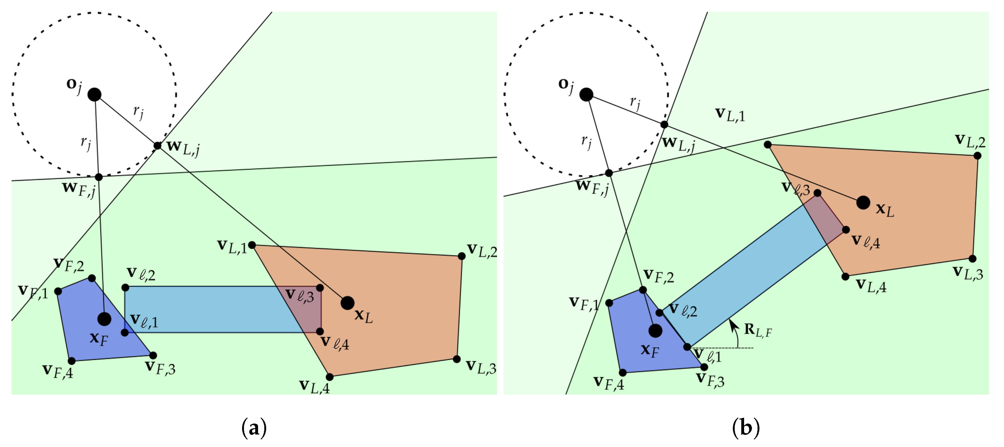
An example of such configuration and the vertices definition is graphically provided later on, in Figure 1.

Given these premises, the final goal of the leader–follower approach is that the two agents will travel along trajectories ${\mathbf{x}}_{•}\left(t\right)$ that are close to the desired reference ${\mathbf{x}}_{•,d}\left(t\right)$. Moreover, the goal of this work consists in the design of a trajectory generation method for the MRS composed of leader and follower, guaranteeing both the load grasping (i.e., the fulfillment of (1)) and the obstacle avoidance (i.e., the fulfillment of (2)). Formally, we aim to determine the desired trajectories ${\mathbf{x}}_{L,d}\left(t\right)$ and ${\mathbf{x}}_{F,d}\left(t\right)$ so that

$$\begin{array}{cc}\hfill & \underset{t\to \infty }{lim}{\mathbf{x}}_{L,d}\left(t\right)={\mathbf{x}}_{L,d}^{*},\hfill \end{array}$$

(4)

$$\begin{array}{cc}\hfill & \parallel {\mathbf{x}}_{F,d}\left(t\right)-{\mathbf{x}}_L\left(t\right)\parallel =d_{L,F},\hfill \end{array}$$

(5)

$$\begin{array}{cc}\hfill & \parallel {\mathbf{v}}_{•,i}\left(t\right)-{\mathbf{o}}_j\left(t\right)\parallel >r_j•=L,F,\ell ,i=1\cdots N_v,j=1\dots M.\hfill \end{array}$$

(6)

In the remainder of the paper, the subscripts L and F are omitted for any quantity when the given observations are valid for both EEs. Moreover, without loss of generality, we assume ${\mathbf{x}}_{L,d}^{*}={\mathbf{0}}_2\in {\mathbb{R}}^2$ in the rest of the work.

3. MPC-Based Strategy

To compute collision-free trajectories for leader and follower, namely ${\mathbf{x}}_{L,d}\left(t\right)$ and ${\mathbf{x}}_{F,d}\left(t\right)$ satisfying (4)–(6), we adopt an MPC-based formulation. Inspired also by the leader–follower framework proposed in [45], the EE positions are assumed to be described by a double integrator model; hence, denoting with ${\mathbf{u}}_L\left(t\right)\in {\mathbb{R}}^2$ and ${\mathbf{u}}_F\left(t\right)\in {\mathbb{R}}^2$ the leader and the follower acceleration inputs, it holds that

$${\ddot{\mathbf{x}}}_L\left(t\right)={\mathbf{u}}_L\left(t\right)\mathrm{and}{\ddot{\mathbf{x}}}_F\left(t\right)={\mathbf{u}}_F\left(t\right).$$

(7)

Introducing also ${\mathbf{v}}_L\left(t\right)={\dot{\mathbf{x}}}_L\left(t\right)$ and ${\mathbf{v}}_F\left(t\right)={\dot{\mathbf{x}}}_F\left(t\right)$ as the leader and follower velocities, the full state of the EEs can be described by

$${\mathbf{q}}_L\left(t\right):=\left[\begin{array}{c}{\mathbf{x}}_L\left(t\right)\\ {\mathbf{v}}_L\left(t\right)\end{array}\right]\in {\mathbb{R}}^4\mathrm{and}{\mathbf{q}}_F\left(t\right):=\left[\begin{array}{c}{\mathbf{x}}_F\left(t\right)\\ {\mathbf{v}}_F\left(t\right)\end{array}\right]\in {\mathbb{R}}^4$$

(8)

which allows to write the dynamics of both the agents as the linear system

$$\dot{\mathbf{q}}\left(t\right)={\mathbf{A}}_c\mathbf{q}\left(t\right)+{\mathbf{B}}_c\mathbf{u}\left(t\right),\mathrm{with}{\mathbf{A}}_c=\left[\begin{array}{cc}{\mathbf{0}}_{2\times 2}& {\mathbf{I}}_2\\ {\mathbf{0}}_{2\times 2}& {\mathbf{0}}_{2\times 2}\end{array}\right]\in {\mathbb{R}}^{4\times 4},{\mathbf{B}}_c=\left[\begin{array}{c}{\mathbf{0}}_{2\times 2}\\ {\mathbf{I}}_2\end{array}\right]\in {\mathbb{R}}^{4\times 2}.$$

(9)

The system model (9) can be discretized with sampling time $T_s\in {\mathbb{R}}_{+}$, thus obtaining

$$\mathbf{q}(t+1)=\mathbf{A}\mathbf{q}\left(t\right)+\mathbf{B}\mathbf{u}\left(t\right),\mathrm{with}\mathbf{A}=e^{{\mathbf{A}}_c{T}_s}\in {\mathbb{R}}^{4\times 4},\mathbf{B}={\int }_0^{T_s}{e}^{{\mathbf{A}}_c\tau }{\mathbf{B}}_c\in {\mathbb{R}}^{4\times 2},$$

(10)

where, with a slight abuse of notation, it holds that $t=h{T}_s$, $h\in \mathbb{N}$.

Given these premises, the cooperative trajectory planning problem is addressed by considering an MPC approach based on the iterative solution of the following optimization problem at each time instant t

$$\begin{array}{ccccc}\hfill {\widehat{\mathbf{u}}}^{*}(·)=& \underset{\widehat{\mathbf{u}}(·)}{argmin}\hfill & J(\widehat{\mathbf{q}}(·),\widehat{\mathbf{u}}(·))\hfill & \hfill & \hfill \end{array}$$

(11)

$$\begin{array}{cccccc}\hfill & \mathrm{subject}\mathrm{to}\hfill & \hfill & \widehat{\mathbf{q}}(k+1)=\mathbf{A}\widehat{\mathbf{q}}\left(k\right)+\mathbf{B}\widehat{\mathbf{u}}\left(k\right)\hfill & \hfill & \left(modeldynamics\right)\hfill \end{array}$$

(12)

$$\begin{array}{cccccc}\hfill & \hfill & & \widehat{\mathbf{q}}\left(0\right)=\mathbf{q}\left(t\right)\hfill & \hfill & \left(initialcondition\right)\hfill \end{array}$$

(13)

$$\begin{array}{cccccc}\hfill & \hfill & & \widehat{\mathbf{q}}\left(k\right)\in \mathcal{X}\left(t\right)\hfill & \hfill & \left(stateconstraint\right)\hfill \end{array}$$

(14)

$$\begin{array}{ccccc}\hfill & & \hfill \widehat{\mathbf{u}}\left(k\right)\in \mathcal{U}& \hfill & \hfill \left(inputconstraint\right)\end{array}$$

(15)

where $k=0\cdots N$ with N being the total prediction horizon samples. In (11)–(15), the vectors $\widehat{\mathbf{q}}\left(k\right):={\left[\begin{array}{cc}{\widehat{\mathbf{x}}}^{\top }\left(k\right)& {\widehat{\mathbf{v}}}^{\top }\left(k\right)\end{array}\right]}^{\top }\in {\mathbb{R}}^4$ and $\widehat{\mathbf{u}}\left(k\right)\in {\mathbb{R}}^2$ represent the state and input prediction respectively, while $\mathcal{X}\left(t\right)$ and $\mathcal{U}$ denote the constraints sets. Given the predicted trajectory $\widehat{\mathbf{x}}(·)$, we generate online at time t the desired trajectory for both leader and follower by considering the first sample of the MPC prediction, namely we have that

$${\mathbf{x}}_d\left(t\right)=\widehat{\mathbf{x}}\left(0\right).$$

(16)

Notice that two different MPC problems need to be considered for the leader and the follower since both the objective and the constraints are different for the two EEs. Moreover, while recalling that completely decentralized approaches are particularly challenging in cooperative transportation tasks based on grasping [6], the strategy outlined here rests on the following points and results in a decentralized scheme.

• Exploiting the described MPC approach, the leader aims at iteratively solving the problem of reaching the target position ${\mathbf{x}}_{L,d}^{*}$, while performing obstacle avoidance (according to (6) given $•=L$) without accounting for the follower. The MPC scheme provides a prediction of the leader trajectory to communicate to the follower.
• After this data exchange, the follower adopts the MPC strategy to compute its trajectory aiming at maintaining the distance $d_{L,F}$ with respect to the leader predicted trajectory and at performing obstacle avoidance for itself and the transported load.

Note that obstacle avoidance for the follower and the load are not considered by the leader to avoid a centralized procedure, which may lead the leader to compute a trajectory that results to be unfeasible from the follower side. However, such case can be detected and handled via the introduction of a proper recovery policy, as explained in Section 5.

Hereafter, taking into account on the optimization problem (11)–(15), we provide a definition for the cost functions $J_L(·)$, $J_F(·)$ and constraints set ${\mathcal{X}}_L\left(t\right)$, ${\mathcal{X}}_F\left(t\right)$, ${\mathcal{U}}_L$, ${\mathcal{U}}_F$ for the leader–follower MPC problem. In particular, the state constraint are time-varying and such that

$${\mathcal{X}}_{•}\left(t\right):={\mathcal{X}}_v\cap {\mathcal{X}}_{•,o}\left(t\right)•=L,F$$

(17)

where ${\mathcal{X}}_v$ is the (same) constraint set on both leader and follower velocity and ${\mathcal{X}}_{•,o}\left(t\right)$ is imposed by the collision avoidance requirement clarified in Section 4.

3.1. Leader Objective Function

The principal goal of the leader is to determine a suitable trajectory such that the error with respect to the final target position ${\mathbf{x}}_{L,d}^{*}$ is minimized. For this reason, accounting for the MPC framework (11)–(15), we consider the quadratic cost function:

$$J_L({\widehat{\mathbf{q}}}_L(·),{\widehat{\mathbf{u}}}_L(·)):=\sum _{k=0}^{N-1}\left({\widehat{\mathbf{q}}}_L^{\top }\left(k\right)\mathbf{W}{\widehat{\mathbf{q}}}_L\left(k\right)+{\widehat{\mathbf{u}}}_L^{\top }\left(k\right)\mathbf{R}{\widehat{\mathbf{u}}}_L\left(k\right)\right)+{\widehat{\mathbf{q}}}_L^{\top }\left(N\right)\mathbf{Z}{\widehat{\mathbf{q}}}_L\left(N\right),$$

(18)

where the gain matrices $\mathbf{W}\in {\mathbb{R}}^{4\times 4}$, $\mathbf{Z}\in {\mathbb{R}}^{4\times 4}$, and $\mathbf{R}\in {\mathbb{R}}^{2\times 2}$ allow to regulate the behavior of the leader in terms of convergence speed towards the target position and control effort.

The function (18) can be rewritten in compact form as

$$J_L({\widehat{\overline{\mathbf{q}}}}_L,{\widehat{\overline{\mathbf{u}}}}_L)={\widehat{\mathbf{q}}}_L^{\top }\left(0\right)\mathbf{W}{\widehat{\mathbf{q}}}_L\left(0\right)+{\widehat{\overline{\mathbf{q}}}}_L^{\top }\overline{\mathbf{W}}{\widehat{\overline{\mathbf{q}}}}_L+{\widehat{\overline{\mathbf{u}}}}_L^{\top }\overline{\mathbf{R}}{\widehat{\overline{\mathbf{u}}}}_L,$$

(19)

by introducing the stacked versions of states, inputs, and corresponding weight matrices, namely

$${\widehat{\overline{\mathbf{q}}}}_L:={\left[{\widehat{\mathbf{q}}}_L^{\top }\left(1\right){\widehat{\mathbf{q}}}_L^{\top }\left(N\right)\right]}^{\top }\in {\mathbb{R}}^{4N},{\widehat{\overline{\mathbf{u}}}}_L:={\left[{\widehat{\mathbf{u}}}_L^{\top }\left(0\right){\widehat{\mathbf{u}}}_L^{\top }(N-1)\right]}^{\top }\in {\mathbb{R}}^{2N},$$

(20)

$$\begin{array}{cccc}\hfill & \overline{\mathbf{W}}=\left[\begin{array}{cc}{\mathbf{I}}_{N-1}\otimes \mathbf{W}& {\mathbf{0}}_{4(N-1)\times 4}\\ {\mathbf{0}}_{4\times 4(N-1)}& \mathbf{Z}\end{array}\right]\in {\mathbb{R}}^{4N\times 4N},\hfill & \hfill & \overline{\mathbf{R}}={\mathbf{I}}_N\otimes \mathbf{R}\in {\mathbb{R}}^{2N\times 2N}.\hfill \end{array}$$

(21)

On the other hand, from the system dynamics (10), for both the leader and the follower, it follows that

$$\widehat{\overline{\mathbf{q}}}=\overline{\mathbf{T}}\widehat{\mathbf{q}}\left(0\right)+\overline{\mathbf{S}}\widehat{\overline{\mathbf{u}}},$$

(22)

where

$$\overline{\mathbf{T}}=\left[\begin{array}{c}{\overline{\mathbf{T}}}_1\\ ⋮\\ {\overline{\mathbf{T}}}_N\end{array}\right]=\left[\begin{array}{c}\mathbf{A}\\ {\mathbf{A}}^2\\ ⋮\\ {\mathbf{A}}^N\end{array}\right]\in {\mathbb{R}}^{4N\times 4},\overline{\mathbf{S}}=\left[\begin{array}{c}{\overline{\mathbf{S}}}_1\\ ⋮\\ {\overline{\mathbf{S}}}_N\end{array}\right]=\left[\begin{array}{cccc}\mathbf{B}& {\mathbf{0}}_{4\times 2}& \cdots & {\mathbf{0}}_{4\times 2}\\ \mathbf{A}\mathbf{B}& \mathbf{B}& \cdots & {\mathbf{0}}_{4\times 2}\\ ⋮& ⋮& \ddots & ⋮\\ {\mathbf{A}}^{N-1}\mathbf{B}& {\mathbf{A}}^{N-2}\mathbf{B}& \cdots & \mathbf{B}\end{array}\right]\in {\mathbb{R}}^{4N\times 2N}.$$

(23)

As a consequence, we can rewrite (18) as

$$\begin{array}{cc}\hfill J_L({\widehat{\mathbf{q}}}_L\left(0\right),{\widehat{\overline{\mathbf{u}}}}_L)& =\frac{1}{2}{\widehat{\overline{\mathbf{u}}}}_L^{\top }\mathbf{H}{\widehat{\overline{\mathbf{u}}}}_L+{\widehat{\mathbf{q}}}_L^{\top }\left(0\right)\mathbf{F}{\widehat{\overline{\mathbf{u}}}}_L+\frac{1}{2}{\widehat{\mathbf{q}}}_L^{\top }\left(0\right)\mathbf{Y}{\widehat{\mathbf{q}}}_L\left(0\right),\hfill \end{array}$$

(24)

with

$$\begin{array}{cc}\hfill \mathbf{H}& =2(\overline{\mathbf{R}}+{\overline{\mathbf{S}}}^{\top }\overline{\mathbf{W}}\overline{\mathbf{S}})\in {\mathbb{R}}^{2N\times 2N},\hfill \end{array}$$

(25)

$$\begin{array}{cc}\hfill \mathbf{F}& =2{\overline{\mathbf{T}}}^{\top }\overline{\mathbf{W}}\overline{\mathbf{S}}\in {\mathbb{R}}^{4\times 2N},\hfill \end{array}$$

(26)

$$\begin{array}{cc}\hfill \mathbf{Y}& =2(\mathbf{W}+{\overline{\mathbf{T}}}^{\top }\overline{\mathbf{W}}\overline{\mathbf{T}})\in {\mathbb{R}}^{4\times 4}.\hfill \end{array}$$

(27)

3.2. Follower Objective Function

The objective of the follower consists in minimizing the distance error with respect to the leader while tracking the shortest path. Since the problem is decentralized, the requirement (5) has to be treated as a desired condition instead of an hard constraint, thus implying the minimization of the squared formation error, defined as follows:

$$e_{L,F}\left(t\right):=\parallel {\mathbf{x}}_L\left(t\right)-{\mathbf{x}}_F{\left(t\right)\parallel }^2-d_{L,F}^2={\parallel {\mathbf{P}}_{\mathbf{x}}\left({\mathbf{q}}_L\left(t\right)-{\mathbf{q}}_F\left(t\right)\right)\parallel }^2-d_{L,F}^2,$$

(28)

given ${\mathbf{P}}_{\mathbf{x}}:=\left[\begin{array}{cc}{\mathbf{I}}_2& {\mathbf{0}}_{2\times 2}\end{array}\right]\in {\mathbb{R}}^{2\times 4}$ and $d_{L,F}$ has been introduced in (1). In detail, the follower aims at solving an MPC optimization problem wherein the cost function is given by a weighted sum of two terms:

• a term accounting for the minimization of the error (28) computed in correspondence to the predicted states ${\widehat{\mathbf{q}}}_L(·)$ and ${\widehat{\mathbf{q}}}_F(·)$, namely

  $$J_{F,1}({\widehat{\mathbf{q}}}_L(·),{\widehat{\mathbf{q}}}_F(·)):=\sum _{k=1}^N{\beta }^k{\left(\parallel {\mathbf{P}}_{\mathbf{x}}\left({\widehat{\mathbf{q}}}_L\left(k\right)-{\widehat{\mathbf{q}}}_F\left(k\right)\right){\parallel }^2-d_{L,F}^2\right)}^2=\sum _{k=1}^N{\beta }^k{\widehat{\mathbf{e}}}_{L,F}^2\left(k\right),$$

  (29)

  where $\beta \in (0,1]\subset \mathbb{R}$ is a decaying weight factor;
• a term accounting for the minimization of the travelled distance in the prediction horizon, namely

  $$J_{F,2}({\widehat{\mathbf{q}}}_L(·),{\widehat{\mathbf{q}}}_F(·)):=\sum _{k=0}^{N-1}{\parallel {\mathbf{P}}_{\mathbf{x}}\left({\widehat{\mathbf{q}}}_F(k+1)-{\widehat{\mathbf{q}}}_F\left(k\right)\right)\parallel }^2.$$

  (30)

Therefore, the cost function associated to the follower results to be

$$J_F({\widehat{\mathbf{q}}}_L(·),{\widehat{\mathbf{q}}}_F(·))=c{J}_{F,1}({\widehat{\mathbf{q}}}_L(·),{\widehat{\mathbf{q}}}_F(·))+J_{F,2}({\widehat{\mathbf{q}}}_L(·),{\widehat{\mathbf{q}}}_F(·)),$$

(31)

where the parameter $c\in {\mathbb{R}}_{+}$ allows to differently prioritize the two aforementioned minimization goal.

Similarly to the leader case, it is possible to rewrite the function (31) as a function of the follower initial state ${\widehat{\mathbf{q}}}_F\left(0\right)$, of the follower predicted control input ${\widehat{\mathbf{u}}}_F$ and of the predicted leader trajectory ${\widehat{\mathbf{q}}}_L\left(k\right)$, $k=1\dots N$. In doing this, we introduce the vectors ${\widehat{\overline{\mathbf{q}}}}_F\in {\mathbb{R}}^{4N}$ and ${\widehat{\overline{\mathbf{u}}}}_F\in {\mathbb{R}}^{4N}$, whose definition is analogous to that of ${\widehat{\overline{\mathbf{q}}}}_L$ and ${\widehat{\overline{\mathbf{u}}}}_L$ in (20). Then, it holds:

$$J_{F,1}({\widehat{\mathbf{q}}}_F\left(0\right),{\widehat{\overline{\mathbf{u}}}}_F,{\widehat{\overline{\mathbf{q}}}}_L)=\sum _{k=1}^N{\beta }^k{\left(\parallel {\mathbf{P}}_{\mathbf{x}}({\widehat{\mathbf{q}}}_L\left(k\right)-{\overline{\mathbf{T}}}_k{\widehat{\mathbf{q}}}_F\left(0\right)-{\overline{\mathbf{S}}}_k{\widehat{\overline{\mathbf{u}}}}_F){\parallel }^2-d_{L,F}^2\right)}^2,$$

(32)

where ${\overline{\mathbf{S}}}_k\in {\mathbb{R}}^{4\times 2N}$ and ${\overline{\mathbf{T}}}_k\in {\mathbb{R}}^{4\times 4}$ are introduced in (23). Moreover, we can further rewrite $J_{F,2}({\widehat{\mathbf{q}}}_L(·),{\widehat{\mathbf{q}}}_F(·))$ as

$$J_{F,2}({\widehat{\mathbf{q}}}_F\left(0\right),{\widehat{\overline{\mathbf{u}}}}_F)={\left({\overline{\mathbf{S}}}^{\prime }{\widehat{\overline{\mathbf{u}}}}_F+{\overline{\mathbf{T}}}^{\prime }{\widehat{\mathbf{q}}}_F\left(0\right)\right)}^{\top }{\overline{\mathbf{P}}}_{\mathbf{x}}^{\top }{\overline{\mathbf{P}}}_{\mathbf{x}}\left({\overline{\mathbf{S}}}^{\prime }{\widehat{\overline{\mathbf{u}}}}_F+{\overline{\mathbf{T}}}^{\prime }{\widehat{\mathbf{q}}}_F\left(0\right)\right),$$

(33)

where ${\overline{\mathbf{P}}}_{\mathbf{x}}={\mathbf{I}}_N\otimes {\mathbf{P}}_x\in {\mathbb{R}}^{2N\times 4N}$ and   

$${\overline{\mathbf{S}}}^{\prime }=\left[\begin{array}{cccc}\mathbf{B}& {\mathbf{0}}_{4\times 2}& \cdots & {\mathbf{0}}_{4\times 2}\\ (\mathbf{A}-{\mathbf{I}}_4)\mathbf{B}& \mathbf{B}& \cdots & {\mathbf{0}}_{4\times 2}\\ ⋮& ⋮& \ddots & ⋮\\ {\mathbf{A}}^{N-2}(\mathbf{A}-{\mathbf{I}}_4)\mathbf{B}& {\mathbf{A}}^{N-3}(\mathbf{A}-{\mathbf{I}}_4)\mathbf{B}& \cdots & \mathbf{B}\end{array}\right]\in {\mathbb{R}}^{4N\times 2N},{\overline{\mathbf{T}}}^{\prime }=\left[\begin{array}{c}\mathbf{A}-{\mathbf{I}}_4\\ \mathbf{A}(\mathbf{A}-{\mathbf{I}}_4)\\ ⋮\\ {\mathbf{A}}^{N-1}(\mathbf{A}-{\mathbf{I}}_4)\end{array}\right]\in {\mathbb{R}}^{4N\times 4}.$$

(34)

Note that, differently from the leader case, the objective function $J_F(·)$ is not quadratic.

3.3. Constraint Sets Definition

To conclude the section, we discuss the constraints that we want to consider regarding the state and control input of both the leader and the follower. From a practical point of view, these are imposed by the actuation limits that implies some bounds both on the velocity and on the acceleration of the EEs.

Formally, within the framework (11)–(15), we can defined the input constraint set as

$$\mathcal{U}:=\{\widehat{\mathbf{u}}\left(k\right)\in {\mathbb{R}}^2:{\mathbf{u}}_{min}\le \widehat{\mathbf{u}}\left(k\right)\le {\mathbf{u}}_{max}\},$$

(35)

where the inequality between vectors is considered component-wise. Equivalently, for each k-th prediction sample, $k=1\cdots N$, it holds that    

$${\mathbf{G}}_a\widehat{\mathbf{u}}\left(k\right)\le {\mathbf{u}}_{lim}\mathrm{with}{\mathbf{G}}_a=\left[\begin{array}{c}-{\mathbf{I}}_2\\ {\mathbf{I}}_2\end{array}\right]\in {\mathbb{R}}^{4\times 2},{\mathbf{u}}_{lim}=\left[\begin{array}{c}-{\mathbf{u}}_{min}\\ {\mathbf{u}}_{max}\end{array}\right]\in {\mathbb{R}}^4,$$

(36)

and, considering the whole prediction horizon, we have that

$${\overline{\mathbf{G}}}_a\widehat{\overline{\mathbf{u}}}\le {\overline{\mathbf{u}}}_{lim}\mathrm{with}{\overline{\mathbf{G}}}_a={\mathbf{I}}_N\otimes {\mathbf{G}}_a\in {\mathbb{R}}^{4N\times 2N},{\overline{\mathbf{u}}}_{lim}={\mathrm{𝟙}}_N\otimes {\mathbf{u}}_{lim}\in {\mathbb{R}}^{4N}.$$

(37)

A similar reasoning can be carried out for constraints affecting the velocity component of the state. Indeed, we consider the velocity constraint set from (17) as:

$${\mathcal{X}}_v:=\{\widehat{\mathbf{q}}\left(k\right)={\left[\begin{array}{cc}{\widehat{\mathbf{x}}}^{\top }\left(k\right)& {\widehat{\mathbf{v}}}^{\top }\left(k\right)\end{array}\right]}^{\top }\in {\mathbb{R}}^4:{\mathbf{v}}_{min}\le \widehat{\mathbf{v}}\left(k\right)\le {\mathbf{v}}_{max}\}$$

(38)

that can be rewritten in terms of control input over the prediction horizon as follows

$${\mathcal{X}}_v=\{\widehat{\overline{\mathbf{u}}}\in {\mathbb{R}}^{2N}:{\overline{\mathbf{G}}}_v\overline{\mathbf{S}}\widehat{\overline{\mathbf{u}}}\le {\overline{\mathbf{v}}}_{lim}-{\overline{\mathbf{G}}}_v\overline{\mathbf{T}}\mathbf{q}\left(0\right)\}$$

(39)

with ${\overline{\mathbf{G}}}_v={\mathbf{I}}_N\otimes {\mathbf{G}}_v\in {\mathbb{R}}^{4N\times 4N}$ and ${\overline{\mathbf{v}}}_{lim}={\mathrm{𝟙}}_N\otimes {\mathbf{v}}_{lim}\in {\mathbb{R}}^{4N}$ given

$${\mathbf{G}}_v=\left[\begin{array}{cc}{\mathbf{0}}_{2\times 2}& -{\mathbf{I}}_2\\ {\mathbf{0}}_{2\times 2}& {\mathbf{I}}_2\end{array}\right]\in {\mathbb{R}}^{4\times 4},{\mathbf{v}}_{lim}=\left[\begin{array}{c}-{\mathbf{v}}_{min}\\ {\mathbf{v}}_{max}\end{array}\right]\in {\mathbb{R}}^4.$$

(40)

Both the input constraint set (35) and the state constraints set (38) are convex.

4. Obstacle Avoidance

In this work, we deal with an environment populated by static and/or dynamic obstacles, thus the cooperative trajectory planning problem has to be faced ensuring also the collision avoidance for the leader, the follower and the transported load. Specifically, as introduced in Section 2, in this work we consider M obstacles. Each j-th obstacle, $j=1\cdots M$, whose position is identified by ${\mathbf{o}}_j\left(t\right)\in {\mathbb{R}}^2$, is associated to a certain radius $r_j\in {\mathbb{R}}_{+}$. It is reasonable to include in the definition of the obstacle radius $r_j$ also possible position measurement errors: formally, by defining the robot position errors as ${\epsilon }_{\mathbf{x},•}\left(t\right)<{\overline{\epsilon }}_{\mathbf{x}}$, $•=L,F$, for each obstacle $j=1\cdots M$ characterized by virtual radius ${\tilde{r}}_j$, we can consider the effective radius $r_j:={\tilde{r}}_j+{\overline{\epsilon }}_{\mathbf{x}}$. Moreover, we recall that collision is avoided with respect to a set of $N_v$ vertices ${\mathbf{v}}_{•,i}\left(t\right)\in {\mathbb{R}}^2$, $i=1\cdots N_v$, $•=L,F,\ell$; with the aim to ease the discussion and without losing in generality, we will assume hereafter that (i) the cardinality $N_v$ of the vertices set is the same for leader, follower, load, namely that they can be modeled with an equal number of boundary points, although different in shape and dimensions; (ii) this definition of vertices (and radius) is adequate to allow for obstacles detection in the considered scenario.

Inspired by the strategy proposed in [46], for both the leader and the follower, we aim at figuring out the largest area that does not contain any obstacle and can be defined with linear constraints. With reference to Figure 1a, in correspondence to any j-th obstacle, we can first consider the point on the circle centered in ${\mathbf{o}}_j\left(t\right)$ closest to the EE position $\mathbf{x}\left(t\right)$, given by:

$${\mathbf{w}}_j\left(t\right)={\lambda }_j\left(t\right)\mathbf{x}\left(t\right)-(1-{\lambda }_j\left(t\right)){\mathbf{o}}_j\left(t\right)\in {\mathbb{R}}^2\mathrm{with}{\lambda }_j\left(t\right)=\frac{r_j}{\parallel \mathbf{x}\left(t\right)-{\mathbf{o}}_j\left(t\right)\parallel }\in \mathbb{R}.$$

(41)

Then, for the EE placed in $\mathbf{x}\left(t\right)$, it is possible to describe the largest half-plane that does not contain the j-th obstacle: this is identified by the line orthogonal to the segment $\mathbf{x}\left(t\right)-{\mathbf{w}}_j\left(t\right)$ and passing through ${\mathbf{w}}_j\left(t\right)$ (green shaded areas in Figure 1). In the light of this fact, j-th obstacle avoidance is guaranteed when the following inequality is satisfied for each i-th vertex, $i=1\cdots N_v$:

$${\mathbf{g}}_{o,j}^{\top }\left(t\right){\mathbf{v}}_{•,i}\left(t\right)\le b_{o,j}\left(t\right),$$

(42)

where $•=L,F,\ell$ and    

$$\begin{array}{cc}\hfill {\mathbf{g}}_{o,j}\left(t\right)& =({\mathbf{w}}_j\left(t\right)-\mathbf{x}\left(t\right))\in {\mathbb{R}}^2,\hfill \\ \hfill b_{o,j}\left(t\right)& ={({\mathbf{w}}_j\left(t\right)-\mathbf{x}\left(t\right))}^{\top }{\mathbf{w}}_j\left(t\right)\in \mathbb{R}.\hfill \end{array}$$

(43)

Given these premises, the collision free area for any robot corresponds to the polyhedron resulting from the intersection of the M half-planes defined as in (42) by taking into account all the obstacles. In detail, we assume that collision avoidance is achieved if each of the $N_v$ vertices belongs to the resulting convex set. Formally, this is ensured by the fulfillment of the following inequality for any $i=1\dots N_v$:

$${\mathbf{G}}_o\left(t\right){\mathbf{v}}_{•,i}\left(t\right)\le {\mathbf{b}}_o\left(t\right),$$

(44)

where $•=L,F,\ell$ and

$${\mathbf{G}}_o\left(t\right)=\left[\begin{array}{c}{\mathbf{g}}_{o,1}^{\top }\left(t\right)\\ ⋮\\ {\mathbf{g}}_{o,M}^{\top }\left(t\right)\end{array}\right]\in {\mathbb{R}}^{M\times 2}\mathrm{and}{\mathbf{b}}_o\left(t\right)=\left[\begin{array}{c}{b}_{o,1}\left(t\right)\\ ⋮\\ b_{o,M}\left(t\right)\end{array}\right]\in {\mathbb{R}}^M.$$

(45)

In order to account for the collision avoidance while solving the cooperative trajectory planning task, we include the constraint (44) in the computation of both ${\widehat{\mathbf{q}}}_L(·)$ and ${\widehat{\mathbf{q}}}_F(·)$. Note that any obstacle position can vary over time but, for the MPC formulation, it is assumed to be fixed during the prediction horizon.

4.1. On the Leader Side

Focusing on the leader, the obstacle avoidance requirement is guaranteed if the constraint (44) is satisfied in correspondence to any element of the set $\{{\mathbf{v}}_{L,i}\left(t\right),i=1\dots N_v\}$. Considering the EE initial state and dynamics, it is possible to verify that, for any $i=1\dots N_v$, the vector ${\widehat{\overline{\mathbf{v}}}}_{L,i}:={\left[\begin{array}{ccc}{\mathbf{v}}_{L,i}{\left(1\right)}^{\top }& \dots & {\mathbf{v}}_{L,i}{\left(N\right)}^{\top }\end{array}\right]}^{\top }\in {\mathbb{R}}^{2N}$ is such that

$${\widehat{\overline{\mathbf{v}}}}_{L,i}={\overline{\mathbf{P}}}_{\mathbf{x}}\left({\overline{\mathbf{T}}}_L{\widehat{\mathbf{q}}}_L\left(0\right)+{\overline{\mathbf{S}}}_L{\widehat{\overline{\mathbf{u}}}}_L\right)+{\overline{\mathbf{s}}}_{L,i},$$

(46)

where ${\overline{\mathbf{s}}}_{L,i}={\mathrm{𝟙}}_N\otimes {\mathbf{s}}_{L,i}\in {\mathbb{R}}^{2N}$. As a consequence, accounting for (45), the obstacle avoidance from the leader side is ensured when the following condition is fulfilled for each $i=1\cdots N_v$

$${\mathcal{X}}_{L,o,i}\left(t\right):=\{{\widehat{\overline{\mathbf{u}}}}_L\in {\mathbb{R}}^{2N}:{\overline{\mathbf{G}}}_o\left(t\right){\overline{\mathbf{P}}}_{\mathbf{x}}\overline{\mathbf{S}}{\widehat{\overline{\mathbf{u}}}}_L\le {\overline{\mathbf{b}}}_o\left(t\right)-{\overline{\mathbf{G}}}_o\left(t\right)({\overline{\mathbf{P}}}_{\mathbf{x}}\overline{\mathbf{T}}{\widehat{\mathbf{q}}}_L\left(0\right)+{\overline{\mathbf{s}}}_{L,i})\},$$

(47)

where

$${\overline{\mathbf{G}}}_o\left(t\right)={\mathbf{I}}_N\otimes {\mathbf{G}}_o\left(t\right)\in {\mathbb{R}}^{MN\times 2N}\mathrm{and}{\overline{\mathbf{b}}}_o\left(t\right)={\mathrm{𝟙}}_N\otimes {\mathbf{b}}_o\left(t\right)\in {\mathbb{R}}^{MN}.$$

(48)

It follows that the leader constraint for obstacle avoidance (17) at time t is given by

$${\mathcal{X}}_{L,o}\left(t\right):=\bigcap _{i=1}^{N_v}{\mathcal{X}}_{L,o,i}\left(t\right),$$

(49)

which results to be a convex set since it is the intersection of (convex) half-planes representing the collision free area.

4.2. On the Follower Side

The reasoning carried out for the leader is valid also for the follower. Specifically, given $i=1\dots N_v$, the following obstacle avoidance condition can be derived

$${\mathcal{X}}_{F,o,i}\left(t\right):=\{{\widehat{\overline{\mathbf{u}}}}_F\in {\mathbb{R}}^{2N}:{\overline{\mathbf{G}}}_o\left(t\right){\overline{\mathbf{P}}}_{\mathbf{x}}\overline{\mathbf{S}}{\widehat{\overline{\mathbf{u}}}}_F\le {\overline{\mathbf{b}}}_o\left(t\right)-{\overline{\mathbf{G}}}_o\left(t\right)({\overline{\mathbf{P}}}_{\mathbf{x}}\overline{\mathbf{T}}{\widehat{\mathbf{q}}}_F\left(0\right)+{\overline{\mathbf{s}}}_{F,i})\}$$

(50)

where ${\overline{\mathbf{s}}}_{F,i}={\mathrm{𝟙}}_N\otimes {\mathbf{s}}_{L,i}\in {\mathbb{R}}^{2N}$ and ${\overline{\mathbf{G}}}_o\left(t\right)$ and ${\overline{\mathbf{b}}}_o\left(t\right)$ are defined as in (48).

The follower is also charged to prevent the transported load from collisions. This requirement, depending on both the leader and follower position, yields to the non linear constraint derived in the following. Consider the unit vector

$$\mathbf{y}\left(t\right):=\frac{{\mathbf{x}}_F\left(t\right)-{\mathbf{x}}_L\left(t\right)}{\parallel {\mathbf{x}}_F\left(t\right)-{\mathbf{x}}_L\left(t\right)\parallel }\in {\mathbb{R}}^2$$

(51)

and the set $\{{\mathbf{s}}_{\ell ,i}\in {\mathbb{R}}^2,i=1\dots N_v\}$ whose elements are the relative positions of the load vertices with respect to the follower position given an arbitrary fixed configuration, e.g., corresponding to the case $\mathbf{y}\left(t\right)={\left[\begin{array}{cc}1& 0\end{array}\right]}^{\top }$. Given the actual position of leader and follower, to ensure the obstacle avoidance by the transported load, we have to consider the position ${\mathbf{v}}_{\ell ,i}\left(t\right)$ of each i-th vertex of the load, $i=1\cdots N_v$. In the light of the given premises, it holds that

$${\mathbf{v}}_{\ell ,i}\left(t\right)=h_{\ell ,i}({\mathbf{x}}_L\left(t\right),{\mathbf{x}}_F\left(t\right))={\mathbf{x}}_F\left(t\right)+{\mathbf{R}}_{L,F}\left(t\right){\mathbf{s}}_{\ell ,i},$$

(52)

where

$${\mathbf{R}}_{L,F}\left(t\right)=\left[\begin{array}{cc}\mathbf{y}\left(t\right)& {\mathbf{y}}_{\perp }\left(t\right)\end{array}\right]\in \mathbb{SO}\left(2\right),\mathrm{with}{\mathbf{y}}_{\perp }\left(t\right)=\left[\begin{array}{cc}0& -1\\ 1& 0\end{array}\right]\mathbf{y}\left(t\right).$$

(53)

According to (42), collision with the j-th obstacle is then avoided if, for any $i=1\cdots N_v$, we have that

$${\mathbf{g}}_{o,j}^{\top }\left(t\right){\mathbf{v}}_{\ell ,i}\left(t\right)\le b_{o,j}\left(t\right),$$

(54)

and this constraint has to be included during the computation of ${\widehat{\mathbf{x}}}_F\left(t\right)$. As a consequence, observing that, for any $k=1\cdots N$, it holds that

$${\widehat{\mathbf{v}}}_{\ell ,i}\left(k\right)={\widehat{\mathbf{x}}}_F\left(k\right)+{\mathbf{R}}_{L,F}\left(t\right){\mathbf{s}}_{\ell ,i}={\mathbf{P}}_{\mathbf{x}}({\overline{\mathbf{T}}}_k{\widehat{\mathbf{q}}}_F\left(0\right)+{\overline{\mathbf{S}}}_k{\widehat{\overline{\mathbf{u}}}}_F\left(k\right))+{\mathbf{R}}_{L,F}\left(t\right){\mathbf{s}}_{\ell ,i},$$

(55)

hence, the constraint set can be rewritten in a more compact fashion accounting for the whole prediction horizon and the complete set of obstacles as:

$$\begin{array}{c}\hfill {\mathcal{X}}_{\ell ,o,i}\left(t\right)=\{{\widehat{\overline{\mathbf{u}}}}_F\in {\mathbb{R}}^{2N}:{\overline{\mathbf{G}}}_o{\overline{\mathbf{P}}}_{\mathbf{x}}\overline{\mathbf{S}}{\widehat{\overline{\mathbf{u}}}}_F\le {\overline{\mathbf{b}}}_o\left(t\right)-{\overline{\mathbf{G}}}_o({\overline{\mathbf{P}}}_{\mathbf{x}}\overline{\mathbf{T}}{\widehat{\mathbf{q}}}_F\left(0\right)-{\overline{\mathbf{s}}}_{\ell ,i}^R)\}.\end{array}$$

(56)

where ${\overline{\mathbf{s}}}_{\ell ,i}^R={\mathrm{𝟙}}_N\otimes \left({\mathbf{R}}_{L,F}\left(t\right){\mathbf{s}}_{\ell ,i}\right)\in {\mathbb{R}}^{2N}$. Finally, the (convex) obstacle avoidance constraint set at the sample time t for the follower is given by the following intersection:

$${\mathcal{X}}_{F,o}\left(t\right):=\bigcap _{i=1}^{N_v}{\mathcal{X}}_{F,o,i}\left(t\right)\cap {\mathcal{X}}_{\ell ,o,i}\left(t\right).$$

(57)

5. Feasibility-Aware Recovery Policy

The decentralized strategy proposed in the previous sections entails that the trajectories of the leader and follower are generated separately, accounting for the diverse constraints characterizing the two robots, whose relative position with respect to the transported load is different. This approach may leads to undesired situations wherein the trajectory computed from the leader yields an infeasible optimum problem for the follower or the outlined follower trajectory produces a formation error that overcomes the inherent elasticity of the grasp structure, thus causing load stresses and eventually load break or grasp detachment. Nonetheless, according to the decentralized approach, it is possible to exploit the reciprocal communication between leader and follower to detect follower-infeasibility conditions and carry out a recovery policy.

Follower-infeasibility conditions generally occur in case of sharp bends or particularly cluttered environments. In the light of this fact, in this section, we propose a heuristic according to which the follower is able to assess if its trajectory in the next $k_{rec}\le N,k_{rec}\in \mathbb{N}$ samples would produce a formation error larger than a predefined threshold $\epsilon \in {\mathbb{R}}_{+}$ and to communicate such information to the leader. Then, the leader will correct its behavior by generating a different (typically slower) trajectory compatible with the follower (and load) dynamics, according to the following conservative optimization functional

$$J_{L,rec}\left({\widehat{\mathbf{q}}}_L(·)\right):=\sum _{k=0}^{N-1}\parallel {\mathbf{P}}_{\mathbf{x}}\left({\widehat{\mathbf{q}}}_L(k+1)-{\widehat{\mathbf{q}}}_L\left(k\right)\right){\parallel }^2=\sum _{k=0}^{N-1}{\parallel {\widehat{\mathbf{x}}}_L(k+1)-{\widehat{\mathbf{x}}}_L\left(k\right)\parallel }^2,$$

(58)

which temporarily replaces (24) in the MPC computation. Algorithm 1, executed at each time instant t, formalizes such introduced heuristic.

Algorithm 1. Recovery policy.

1: ${\widehat{\overline{\mathbf{x}}}}_L\leftarrow$ MPC leader prediction considering $J_L(·)$ in (18) 2: ${\widehat{\overline{\mathbf{x}}}}_F\leftarrow$ MPC follower prediction considering $J_F(·)$ in (31) 3: if$\parallel {\widehat{\mathbf{x}}}_L\left(k\right)-{\widehat{\mathbf{x}}}_F{\left(k\right)\parallel }^2-d_{L,F}^2>{\epsilon }^2$ for any $k=1\cdots k_{rec}$ then 4: ${\widehat{\overline{\mathbf{x}}}}_{L,rec}\leftarrow$ MPC leader prediction considering $J_{L,rec}(·)$ in (58) 5: ${\widehat{\overline{\mathbf{x}}}}_{F,rec}\leftarrow$ MPC follower prediction considering $J_F(·)$ in (31) computed for ${\widehat{\overline{\mathbf{x}}}}_{L,rec}$ 6: ${\mathbf{x}}_{L,d}\left(t\right)\leftarrow {\widehat{\mathbf{x}}}_{L,rec}\left(0\right)$ 7: ${\mathbf{x}}_{F,d}\left(t\right)\leftarrow {\widehat{\mathbf{x}}}_{F,rec}\left(0\right)$ 8: else 9: ${\mathbf{x}}_{L,d}\left(t\right)\leftarrow {\widehat{\mathbf{x}}}_L\left(0\right)$ 10: ${\mathbf{x}}_{F,d}\left(t\right)\leftarrow {\widehat{\mathbf{x}}}_F\left(0\right)$ 11: end if

6. Numerical Results

This section is devoted to the validation of the proposed MPC solution for the trajectory planning problem within the context of cooperative transportation in a cluttered environment, as described in Section 2. It has already been highlighted how such application involves the accomplishment of three distinct and simultaneous goals, which need to be consistently accommodated by the control action: the leader is required to reach the target position ${\mathbf{x}}_{L,d}^{*}$, the follower is required to maintain the distance $d_{L,F}$ from the leader, both the agents are required to avoid the obstacles and the follower also needs to prevent the transported load from collisions.

In the light of this fact, to assess the performance of the proposed solution, we account for the following three metrics:

• the leader position ${\mathbf{x}}_L\left(t\right)$ with respect to the target position ${\mathbf{x}}_{L,d}^{*}$, given the assumption ${\mathbf{x}}_{L,d}^{*}={\mathbf{0}}_2$;
• the quadratic formation error $e_{L,F}\left(t\right)={\parallel {\mathbf{x}}_L\left(t\right)-{\mathbf{x}}_F\left(t\right)\parallel }^2-d_{L,F}^2$ introduced in (28);
• the index $d_{•,min}\in \mathbb{R}$ defined as follows

  $$d_{•,min}=\underset{\begin{array}{c}i=1\cdots N_v\\ j=1\cdots M\end{array}}{min}\left(\parallel {\mathbf{v}}_{•,i}\left(t\right)-{\mathbf{o}}_j\left(t\right)\parallel -r_j\right),•=L,F,\ell ,$$

  (59)

  and corresponding to the distance between the closest pair of i-th vertex and j-th obstacle boundary. Note that this involves the obstacle radius so the collision is avoided for positive values of $d_{•,min}$.

Hereafter, we report the results for three different obstacles configurations:

(i)

$M=2$ large static identical obstacles, forming a narrow passage;

(ii)

$M=3$ static obstacles, of different size;

(iii)

$M=24$ obstacles, where one obstacle can move, while the other are fixed but characterized by different radii. Some of these obstacles, in particular, are placed contiguously to each other so as to form a narrow corridor.

For all the configurations, the leader and follower parameters are reported in

Table 1. Numerical scenario parameters.

	Leader	Follower
Scenario
${\mathbf{u}}_{max}$ [m/s2]	0.8 ${\mathrm{𝟙}}_2$	2${\mathrm{𝟙}}_2$
${\mathbf{v}}_{max}$ [m/s]	0.2${\mathrm{𝟙}}_2$	1${\mathrm{𝟙}}_2$
$d_{F,L}$ [m]	1	1
$N_v$	20	20
${\left\{{\mathbf{s}}_i\right\}}_{i=1}^{N_v}$[m]	${\left\{0.32\left[\begin{array}{c}cos\left(0.3i\right)\\ sin\left(0.3i\right)\end{array}\right]\right\}}_{i=1}^{N_v}$	${\left\{\left[\begin{array}{c}0\\ 0\end{array}\right]\right\}}_{i=1}^{N_v}$
${\left\{{\mathbf{s}}_{\ell ,i}\right\}}_{i=1}^{N_v}$ [m]		$\left\{\left[\begin{array}{c}-0.2-d_{F,L}\\ -0.2-d_{F,L}\end{array}\right],\left[\begin{array}{c}0.2\\ -0.2\end{array}\right],\left[\begin{array}{c}0.2\\ 0.2\end{array}\right],\left[\begin{array}{c}-0.2-d_{F,L}\\ 0.2\end{array}\right]\right\}\cup {\left\{\left[\begin{array}{c}0\\ 0\end{array}\right]\right\}}_{i=5}^{N_v}$
Leader objective function
$\mathbf{W}$	${\mathbf{I}}_4$	–
$\mathbf{R}$	$0.9{\mathbf{I}}_2$	–
$\mathbf{Z}$	${\mathbf{I}}_4$	–
Follower objective function
c	–	5000
$\beta$	–	0.95
Leader recovery objective function
$\epsilon$ [m]	0.01	–
$k_{rec}$	3	–

.

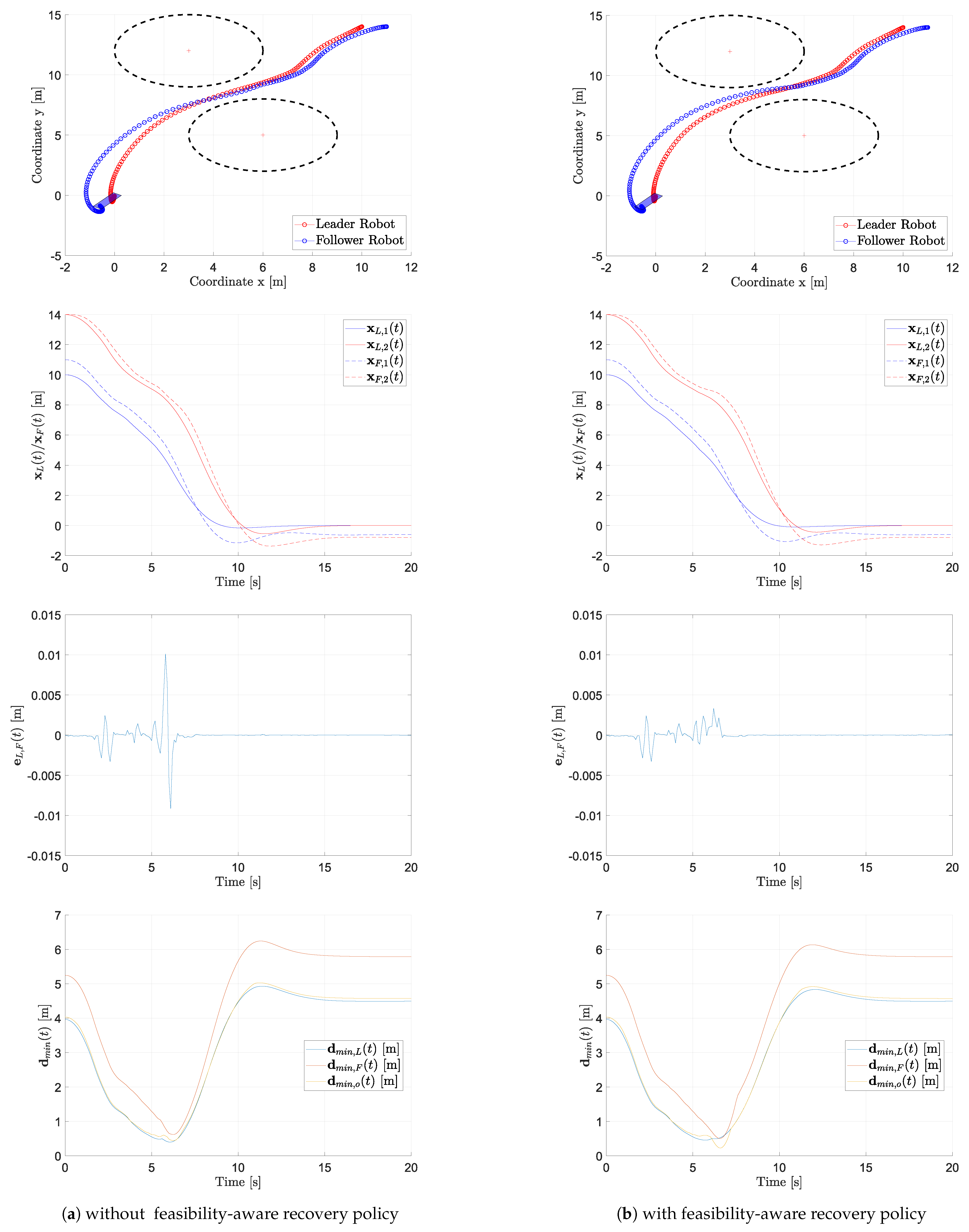
Configuration (i)

Figure 2 reports the outcome of one of the performed numerical simulation, providing both an overview of the scenario and of the task evolution and the behavior of the performance metrics. The two columns refer respectively to the case in which the recovery policy of Section 5 is considered (right) or not (left). For both cases, we report the planar trajectory of the leader and follower (first panel, at the top) as well as the trend of their position components (second panel), the trend of the formation error $e_{L,F}\left(t\right)$ (third panel) and the trend of the index $d_{•,min}$ for $•=L,F,o$ (fourth panel).

The reported plots allow us to assess the performance of the proposed MPC-based trajectory generation strategy and, in particular, to appreciate the benefit deriving from the introduction of the feasibility-aware recovery policy. Indeed, it is possible to observe that, both with and without implementing the recovery policy, the leader converges towards the target position (second panel in Figure 2). However, the employment of the recovery policy is motivated by the rapid increase of the leader–follower formation error at approximately $t=6$ s, in correspondence to the narrow passage by the two obstacles: the modification of the MPC optimization function for the leader is effective in leading to a smaller formation error (third panel) at the cost of a slightly slower convergence speed. Finally, the plots in the bottom panel confirm that the agents and the load are able in both cases to keep the desired distance from the obstacles. As a further remark, we notice that the challenging region to overcome is the one closest to the obstacles, where the obstacle avoidance constraints are modified more quickly.

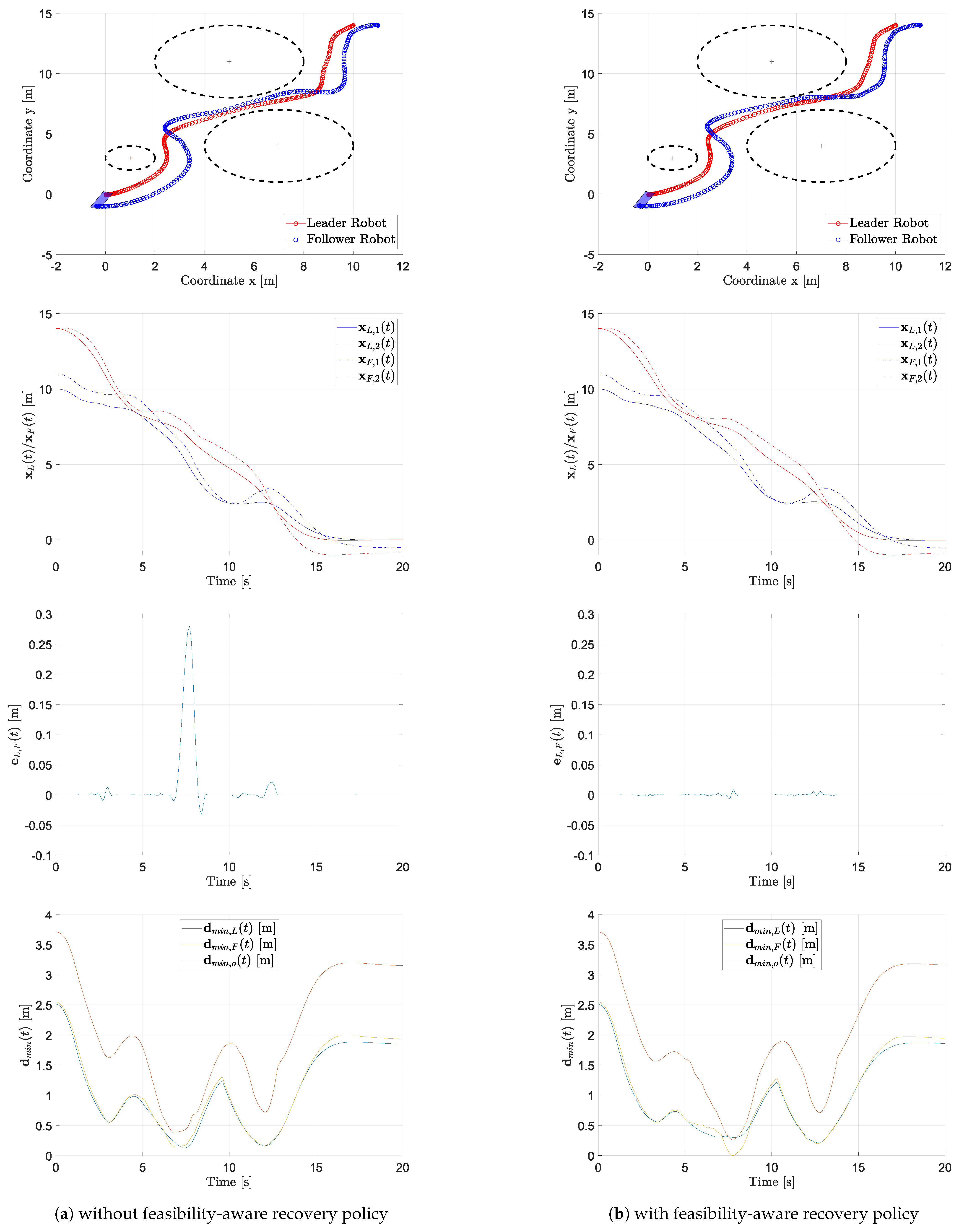
Configuration (ii)

This configuration differs from the previous because of the presence of an additional (static) obstacle, whose position is such to require an aggressive maneuver by the leader–follower system.

This scenario behavior is highlighted by the results reported in Figure 3. As in the previous case, from the first and second panels, we observe that the leader can reach its target position, both implementing the recovery policy (Figure 3b) and not implementing the recovery policy (Figure 3a). As pointed out in the previous case, nearby the obstacles the linear constraints change very quickly and in this case it is more difficult for the follower to keep the formation error low: again, the constraints imposed by the two large obstacles with the additional presence of that along the predicted trajectory for the MRS, leads to a peak in the $e_{L,F}$ metrics value, because the follower need to re-arrange its position accounting for both its own occupancy and that of the load. In this case, the feasibility-aware recovery policy turns out to be fundamental to limit the formation error: from the third panel we notice that the $e_{L,F}$ is drastically reduced by slowing down the formation speed when needed. Finally, obstacle avoidance is granted in this case as well. Note that at around $t=8$ s the load is very close to the constraint limit, which nonetheless does not raise a risk for physical collision if the radius accounts also for a certain safety margin.

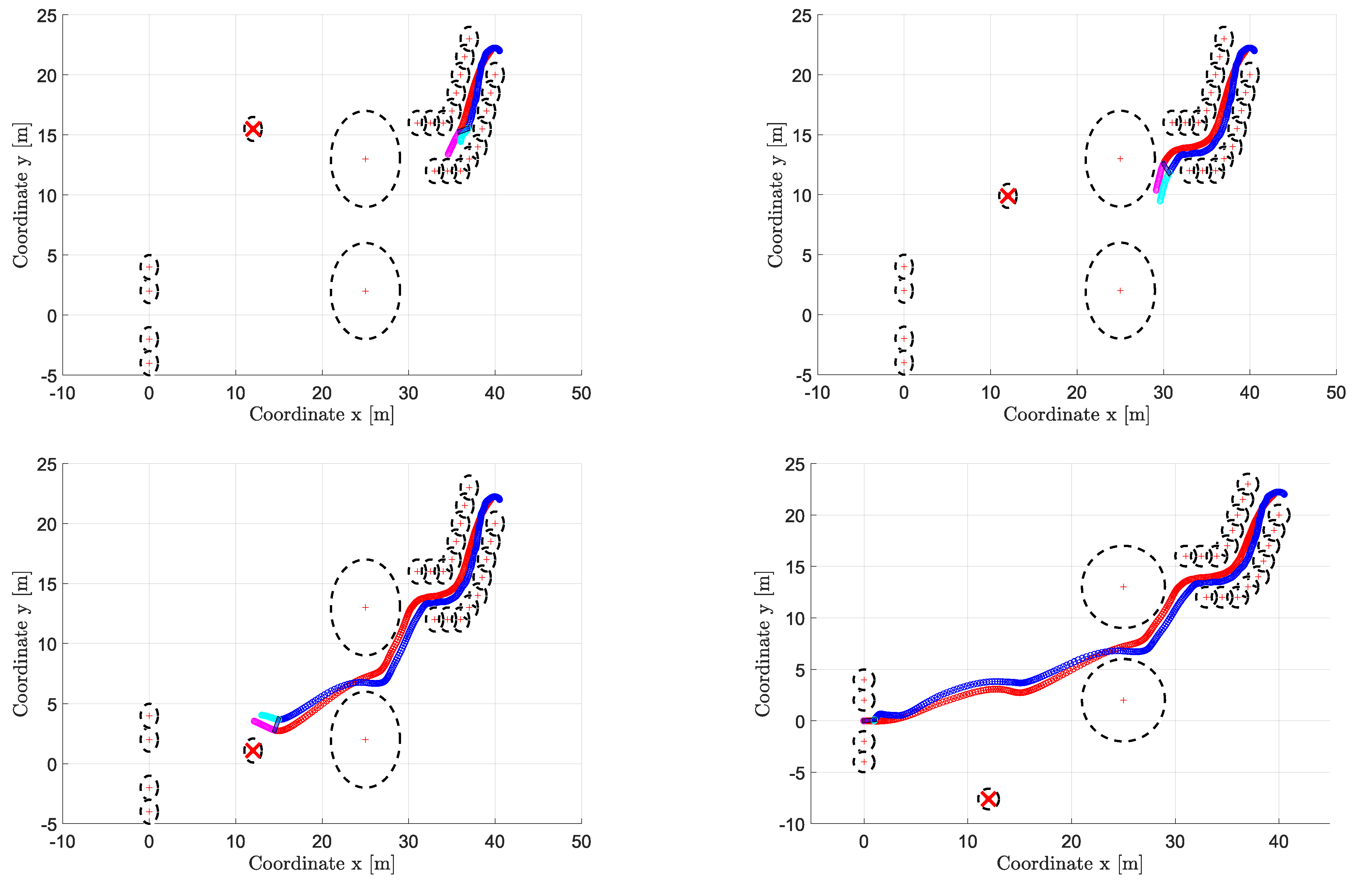
Configuration (iii)

The last configuration here presented includes 23 static obstacles (two bigger than the others) and a dynamic obstacle (in total $M=24$). In particular, the former are arranged so as to form a corridor and two narrow passages, one of which in correspondence to the target position; the moving obstacle, instead, travels along an unknown trajectory in the area in front of the target, as shown in Figure 4.

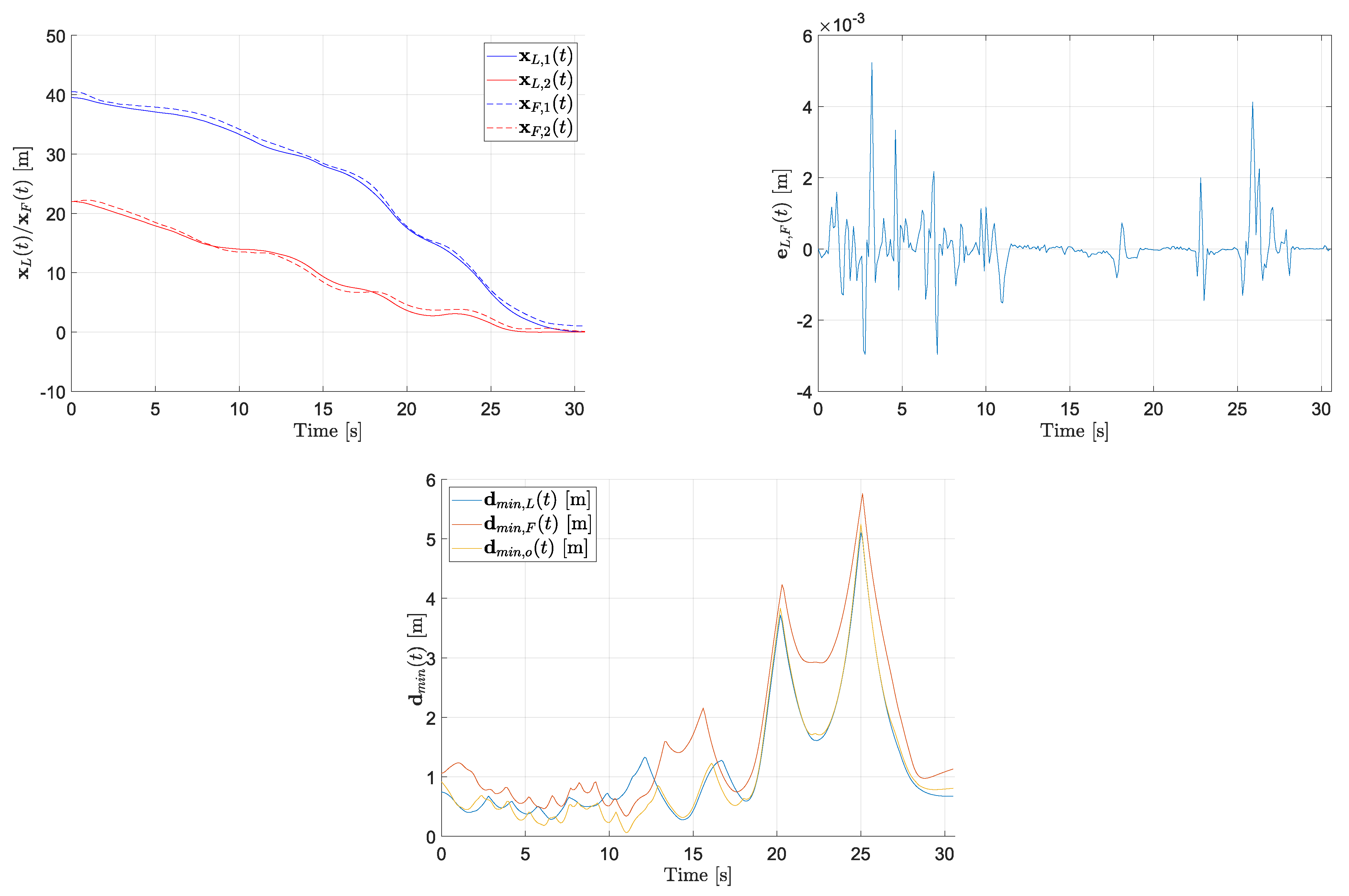
In this case, only the control with the recovery policy is discussed: the plots in Figure 4 show four snapshots of the MRS behavior, specifically at $t=8$ s, $t=13.5$ s, $t=22.5$ s, and $t=30$ s, and the performance index results reported in Figure 5 confirm the effectiveness of the proposed trajectory planning solution. As a general comment, in such a complex scenario the implementation of the feasibility-aware recovery policy ensures both the minimization of the formation error (note the different scale w.r.t. to the plots in Figure 2 and Figure 3) and the collision avoidance while fulfilling the velocity constraints. In detail, we can well appreciate four dynamic phases on which to spend some comments:

• t = 0–12 s: the MRS is travelling the corridor abiding several constraints, with an impact on the performance index (59), which is low; moreover, the effects of the control of leader and follower on the load show in this phase a relatively higher formation error.
• t = 12–20 s: the MRS is going through the narrow passage made of the two large obstacles, being very close to the upper obstacle at $t=14.5$ s and to the lower one at $t=18$ s.
• t = 20–25 s: the motion is now in the open area where the main issue is represented by the presence of the mobile obstacle, which is intersecting the estimated MRS trajectory at $t=21$ s, thus causing the leader to react by planning a motion correction slightly upwards.
• t = 25–30 s: the final phase is characterized by the maneuver of MRS and the action of the follower on the load, rotating it in order to enter the goal area horizontally (hence the noisy behavior of the formation error).

7. Conclusions

Motivated by the cutting-end research and application trends within MRS scenarios, we present a decentralized strategy to perform cooperative transportation by two mobile ground robots. The procedure is based on a leader–follower scheme and exploits an MPC approach running in parallel on both agents: the leader, basing on its own state, has the task of designing a potentially effective collision free trajectory for the whole MRS towards the goal. The follower, instead, has to accommodate the leader command with its proper and the load’s constraints to ensure the overall task transportation feasibility. In case the trajectory computed by the leader is not feasible for the follower/load movement, the leader is able to switch to a conservative recovery policy that ensures task completion. The proposed approach is discussed formally and the overall control procedure is validated in a simulation framework that includes different scenarios, highlighting the effectiveness of the technique and the role of the proposed recovery policy.

Interestingly, many different aspects that are worth to be studied stem from the methodology presented in this work, which mainly regard the control of the interaction between the transporting robots and the load, the regulation of the load orientation at the target position, the management of non-convex obstacles and of very dynamic environments.