Multi-Agent Collaborative Path Planning Based on Staying Alive Policy †


Robotics Team, Department of Computer, Electrical and Space Engineering, Luleå University of Technology, SE-97187 Luleå, Sweden
*
Author to whom correspondence should be addressed.
†
This paper is an extended version of our paper published in Koval, A., Mansouri S. S., Nikolakopoulos G. Online Multi-Agent Based Cooperative Exploration and Coverage in Complex Environment. In Proceedings of the 2019 18th European Control Conference (ECC), Naples, Italy, 25–28 June 2019.
Robotics 2020, 9(4), 101; https://0-doi-org.brum.beds.ac.uk/10.3390/robotics9040101
Submission received: 12 October 2020
/
Revised: 18 November 2020
/
Accepted: 20 November 2020
/
Published: 28 November 2020
(This article belongs to the Special Issue Optimal Robot Motion Planning)
Abstract
:Modern mobile robots tend to be used in numerous exploration and search and rescue applications. Essentially they are coordinated by human operators and collaborate with inspection or rescue teams. Over the time, robots became more advanced and capable for various autonomous collaborative scenarios. Recent advances in the field of collaborative exploration and coverage provide different approaches to solve this objective. Thus scope of this article is to present a novel collaborative approach for multi-agent coordination in exploration and coverage of unknown complex indoor environments. Fundamentally, the task of collaborative exploration can be divided into two core components. The principal one is a sensor based exploration scheme that aims to guarantee complete area exploration and coverage. The second core component proposed is a staying alive policy that takes under consideration the battery charge level limitation of the agents. From this perspective the path planner assigns feasible tasks to each of the agents, including the capability of providing reachable, collision free paths. The overall efficacy of the proposed approach was extensively evaluated by multiple simulation results in a complex unknown environments.
1. Introduction
For the last years, the number of applications where mobile robots collaborate with humans [1] dramatically increased. Mainly, this is due to advances in batteries, powerful computation boards, and miniaturization of sensors. Robust and sophisticated mobile robots became a vital tool in human life, such as smart wheelchairs for disabled people [2], in autism therapy [3], and for tour-guiding [4]. Moreover, they are used in disaster search and rescue missions [5], utility inspection [6], crop monitoring [7], etc. Depending on mission requirements, mobile robots could be equipped with different types of sensors or actuators that depend on the mission objectives. Their assistance in inspection, search, and rescue missions, and the exploration of unknown areas plays crucial role and provides benefits to human operator safety, decision making, fast exploration, three-dimensional (3D) reconstruction of the environment, and providing localization [5]. In these contexts, mobile robots could be equipped with depth cameras or laser range finders that are used for navigation and situational awareness [8,9].
Most of previous works study the deployment of single robot scenarios [10,11,12]; however, in the majority of the real worlds size problems, such as exploration and coverage of large areas [13], there is a need of multiple robots for guaranteeing successful mission [14]. This arises multiple challenges and increases the complexity of the problem such as collision free deployment of team of robots [15], guaranteeing the full coverage of the explored area, while taking into account the physical limitation of each robot, such as the remaining battery operating time and defining coordination between robots. This requires theoretical, practical, and technological contributions towards the deployment of team of robots in real-life scenarios.
Nowadays, exploration and complete coverage of unknown areas is receiving a considerable high research attention. In the following survey articles [16,17], numerous approaches have been proposed for solving this demanding task, while, in general, the task of exploration could be divided into online and offline approaches. The offline algorithms typically require prior knowledge of the environment that in many real life use-cases is not available. On the contrary, online algorithms or sensor-based algorithms can operate without prior knowledge of the environment; however, the outcome in this case is reaching sub-optimal solutions.
Towards the second direction, one of the most known online algorithms for achieving a complete area coverage is based on the Boustrophedon motion [18]. For example, in [19], this algorithm was utilized together with the dynamic programming for a single mobile root. The authors in [20] proposed an algorithm that incrementally decomposed the unknown environment into cells and the corresponding online path planning relied on data from a laser scanner. In [21] it was suggested the worst case scenario model for planning coverage paths that could be applicable for GPS enabled robots, while the work in [22] suggested using a genetic algorithm for achieving a coverage based path planning. In [23], a path planning algorithm was proposed that was able to minimize the number of turns or repetitions in order to increase the overall algorithmic efficiency. However, one of the main shortcomings of these works was the fact that the physical limitations of the utilized robots, from a power consumption point of view, have not been taken under consideration, while, at the same time, was focusing on the single robot use-case. On the contrary, studies as those in [24,25,26] suggested approaches that considered limited robot resources, but were still solving the coverage problem only for the case of a single agent.
In the field of collaborative area coverage, significant contributions have been reported in [27,28,29,30], where it was suggested an online coverage algorithm and a cost function was proposed based on distance measurements; however, the reality of a limited battery operating time has not been taken under consideration. In [31], it was proposed a cooperative mapping algorithm, based on heterogeneous robots and the established algorithm in [18,32,33] with an explorer-coverer architecture. As was presented, during the stage of the cooperative exploration, the agents discover the unknown region boundaries, while the task finishes when the Reeb Graph [34] is complete. In this approach, the coverers execute a back-and-forth motion (sweeping motion). For this scenario, an auctioning mechanism is used for the task re-allocation. However, in both works the authors do not consider a limited battery operating time. Moreover, the approach suggested in [35] uses multiple heterogeneous unmanned aerial vehicles for the area partitioning, while, in this case, the proposed computational algorithm requires future optimizations and it is an offline approach.
In this article, the multi-agent area coverage of the unknown two-dimensional (2D) environment is studied, while taking under consideration the limited battery operating time of the agents. The main contribution of this article stems from the deployment of multiple agents in complex indoor environment with a sensor based approach, where the online exploration method is inspired from the Boustrophedon motion (BM) proposed in [18,28] and expanded by considering multiple agents with a limited battery operating time. Additionally, in order to determine backtracking points, the detection conditions in [36] have been adapted to meet the overall mission requirements. The evaluation of the proposed online method in computer simulation scenarios, inspired from real-world non-convex areas with multiple branches will demonstrate its efficacy for online area coverage of the unknown environment, while providing well-balanced work distribution between agents.
The rest of the article is structured, as follows. Initially, the notations and preliminaries are presented in Section 2, while the proposed multi-agent based cooperative exploration and coverage scheme is established in Section 3. The simulation results are presented in Section 4, and finally the article is concluded in Section 5.
2. Notation and Preliminaries
In the proposed method, each agent covers a squared area with a length, where it is assumed that the agent is placed in the middle of it and as the result of the exploration task a grid map is obtained with the same resolution. Furthermore, and without a loss of generality, it is assumed that the movement of the agent is defined with four directions, specifically North, South, East, and West, and rotation around its geometric centre. In each step, the agents can move in a fixed distance l and rotate by . The pose of the agent can be defined by the vector, where are the coordinates and is the heading at the time instant , with the corresponding kinematic equations being denoted by:
The workspace W and its coverage model M are in , while the sets C within the workspace are denoted as and and , , and denote the free space, obstacles, and global backtracking points sets, respectively. The transpose of a matrix is denoted as . The superscripts , and , denote a charging point (station), a backtracking point and a minimum value correspondingly. The energy is denoted as a scalar value, while is the energy level of the agent i and, at the k time instant, is the energy spent for the translation from to . Furthermore, a lost agent is defined as , a blocked position as , and an unblocked position as . The path from to is defined as , where is the position of the agent and is set of all the agent positions. Furthermore, denotes the Euler distance between the position and . With will be denoted the number of agents. Finally, is the sensor model and operator ∖ denotes set subtraction.
3. Cooperative Exploration and Coverage Scheme
In the proposed methodology, it is assumed that the environment has only one entrance, which is considered to be the starting point. It is also assumed that the discovered branches/areas have at least the same width as the agent’s sweep step. At the starting point, all of the agents are looking towards the unknown area and in each iteration the agent completely covers the next cell. The overall proposed exploration scheme contains three components: (a) an exploration method, (b) a staying alive policy, and (c) a path planner, while these parts will be analysed in the sequel.
3.1. Exploration Method
In the proposed methodology, the unknown areas of the workspace W are incrementally discovered through the Boustrophedon motion [28], so that the agent translates forward or backward, exploring the surrounding space, until it reaches a blocked position and rotates to alter the direction of the translation. During exploration, each agent at each step performs sensing of the surrounding environment, denoted by , according to the sensor model that is defined as:
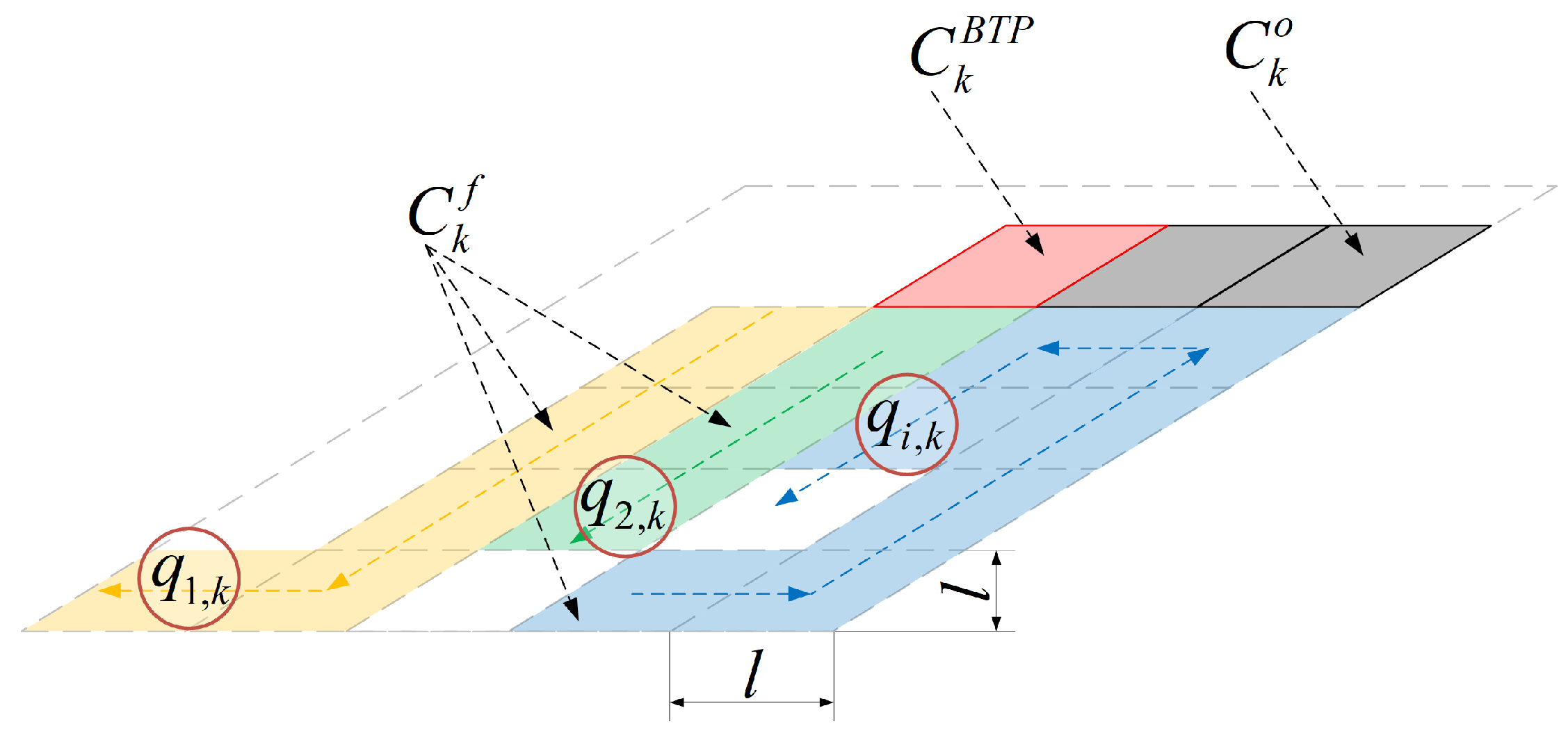
where —corresponds to each adjacent area around the agent. After the completion of the overall unknown area, it will be represented as a grid map (global map, coverage model) M [36] with discovered free space and obstacles , with the overall architecture being depicted in Figure 1.
Relying on the , the agents perform the BM according to the algorithm presented in Algorithm 1 and detect the corresponding backtracking points (BTPs) that generally can be any agent’s neighbouring point that satisfies the following statement , while it should be mentioned that these points are utilized for the detection of the adjacent unknown regions if existing.
| Algorithm 1 Boustrophedon motion (BM) algorithm |
| Require:, M |
|
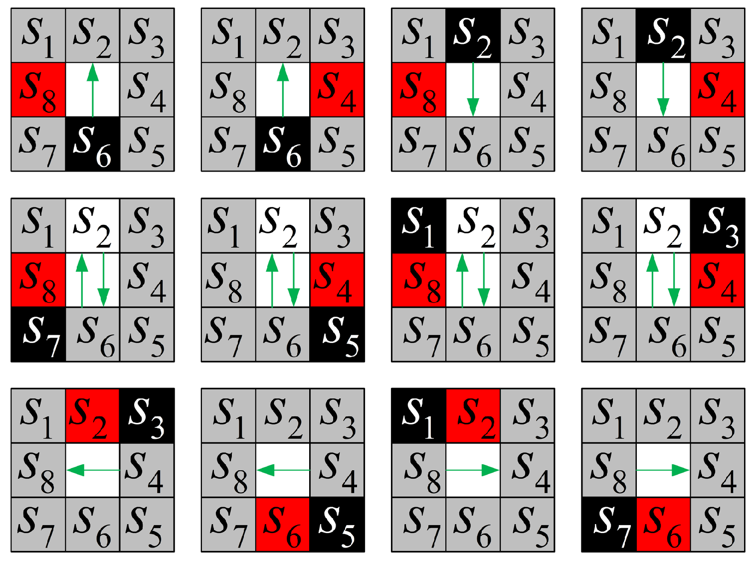
Without a proper selection mechanism for the BTPs, the total agent’s path can have a lot of unnecessary transitions that will increase the overall distance and exploration time. This article proposes the novel idea in order to reduce the number of BTPs unlike, as appeared in [18,36], where a robot detects BTPs from the accumulated knowledge (covered path) only when it reaches blocked condition and uses all eight neighbouring cells of a tile to detect BTP. In the proposed approach, sensor measurements are used to detect BTPs at each step, but novel detection conditions are proposed, as depicted in Figure 2, where the black tiles denote obstacles, the red tiles correspond to BTPs, and the grey tiles are free areas that are not considered for detection, while the green arrows indicate the agent’s motion direction, when the BTP can be detected. The agent is placed in the middle (white tile) and the neighbouring cells are sensor measurements, unlike the approach proposed in [18,36], where the backtracking point is in the middle. For making the overall approach more clear, let us consider left condition in the middle row of Figure 2, which uses three out of the eight measured points to calculate the BTP. In this case, the green arrows indicate that the BTP can be detected, while moving to the North or to the South. After obtaining the sensor measurements , it results that and . To obtain the motion direction, the should be considered and, of the forward or backward direction is not blocked, then . Depending on the complexity of the unknown area, the number of backtracking points could be proportional to the number of agent steps. Therefore, in the proposed work, we consider that, while the agent performs BM, it discovers and covers BTPs, so the already visited BTPs are removed from the agent’s BTP stack, and this operation can be defined as:
At the same time, each agent locally operates based on his own BTP stack and it globally uses data from the global BTP stack shared among the agents as if , and it relies on its sensor measurements to provide non-overlapping coverage paths. In case there are more agents than BTPs, a free agent is waiting for the first available BTP in the global stack. The global map of discovered area M (coverage model) is updated in each iteration from all agents, unless the agent makes a turn or holds its position. The full coverage of the unknown area is achieved when the and presented as map model M.
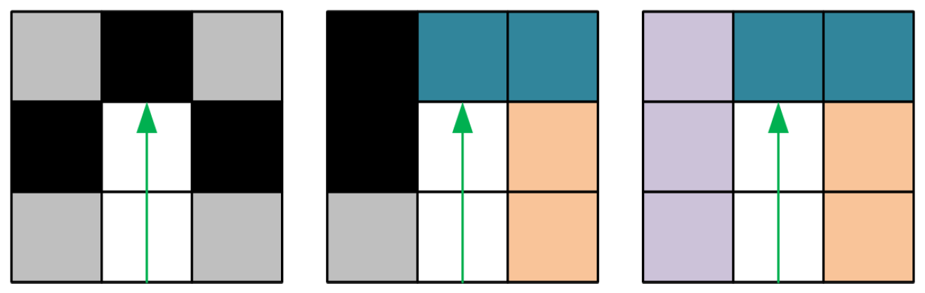
In the proposed approach, it is considered that, while performing BM, the agents never revisit discovered areas unless they reach a blocked position . Such an example is depicted on the Figure 3, where the different blocked conditions are shown and there is a need for generating the path from the actual agent’s position to the next available BTP.
3.2. Staying Alive Policy
In the proposed scheme, it is considered that all of the agents are battery powered and have limited operation time [37]. Mission planning without considering this limitation may result in the loss of agents [38] and even result in a mission failure. Thus, in this work, the policy for staying alive for all agents is introduced.
Agent’s transition energy is defined as and it is evaluated at each BM step (iteration), as:
where corresponds to the agent’s minimum energy spent per one iteration. The energy consumption for each agent can be defined as:
where corresponds to the actual battery energy level, where a full charge denotes a value of and the critical charge denotes value that is below . The overall algorithm for staying alive policy (SAP) is shown in Algorithm 2, where the required energies and are calculated using Equation (4).
| Algorithm 2 Staying alive policy algorithm |
| Require:, |
|
Moreover, in case the agent requires charging , the path planner that is presented in the Section 3.3 will generate a collision free path to BTP or to the charging station.
3.3. Path Planner
In general, the agents perform an exploration task that is based on BM. However, when the battery level of an agent is low, which is denoted from or the agent is blocked , the agent should navigate to the charging station , or the closest BTP , respectively. Thus, a Probabilistic Roadmap (PRM) planner [39] is implemented in order to generate collision free paths from to based on the discovered map M.
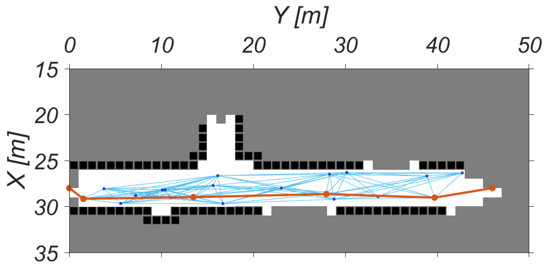
The PRM is based on a non-directed graph that contains all possible trajectories that are derived from the occupancy grid. Generally, the PRM path planner has two phases: learning and query. During first phase it constructs a roadmap of a free space as an non directed graph, while in the second phase the method tries to connect the and the positions by a corresponding path. Figure 4 shows the generated non-direct graph by blue lines and corresponding path in the orange.
Furthermore, the path planner algorithm is presented in Algorithm 3, where “” denotes equality. It requires the current position of the agent , the position of charging station , and the set of BTPs . Subsequently, in the case of all paths to BTPs are calculated (Figure 5a),while the BTP with a minimum length of the path is selected for the agent to visit. However, if the agent’s battery level is not sufficient, for reaching to based on Algorithm 2, the agent should navigate to the charging station (Figure 5b). In this case , only one path from to the charging station is obtained.
| Algorithm 3 Path planner |
| Require:, , |
|
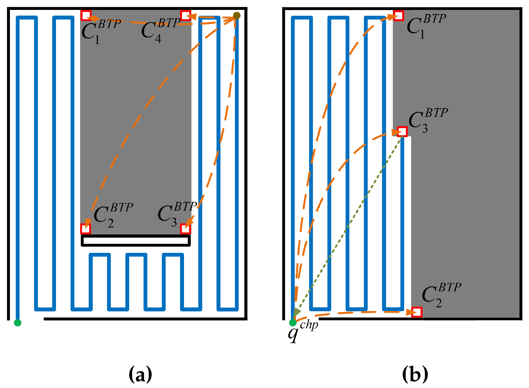
Figure 5 depicts examples of these two cases. On the left image (corresponds to the first case) the agent starts BM and while moving discovers free space and BTPs. Accordingly, at first it discovers , after , and finally . After a while, the agent reaches its blocked position , which means that this BM is finished. From this point, there are four possibilities to continue exploration. The PRM planner will calculate paths and their distances to each BTP and will send an agent to the nearest one to continue exploration. On the right image (corresponds to the second case), while conducting BM agents’ charge level became low (signalized from the staying alive policy), so the agent has to visit charging point . The path is generated by a PRM planner. After recharging, PRM planner will provide the shortest path to the agent to continue exploration from three available possibilities (, , and ).
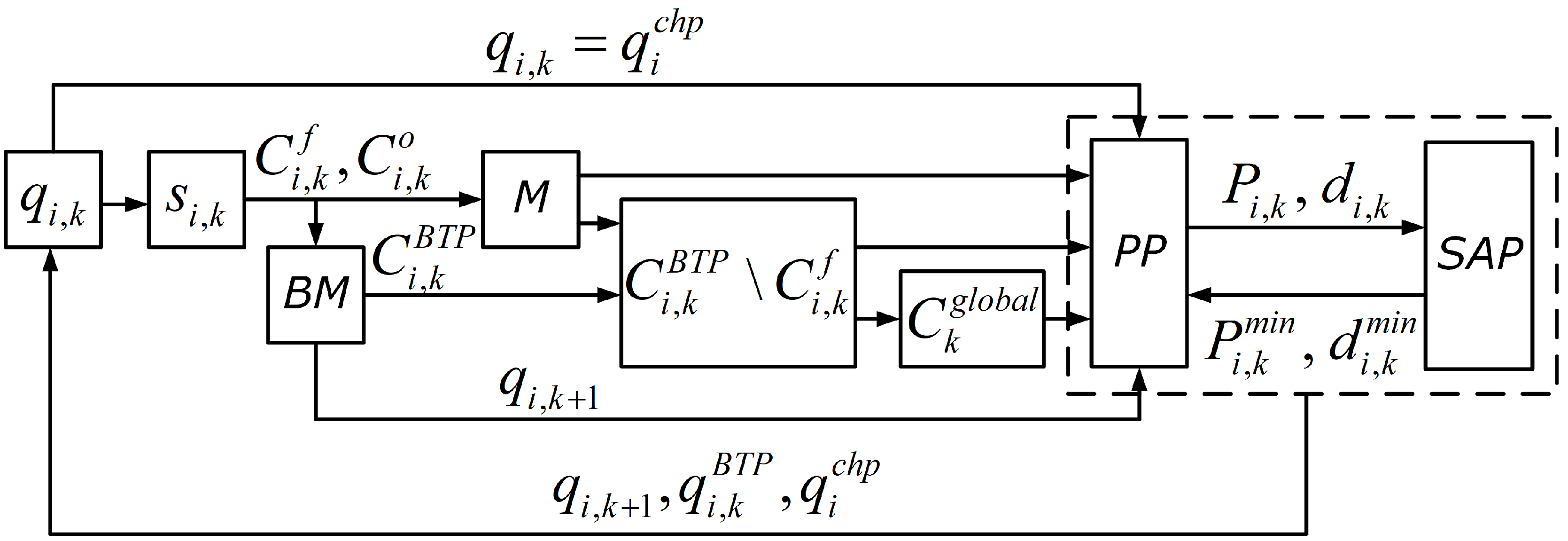
Overall, the final cooperative exploration and coverage scheme is summarized in Algorithm 4 and Figure 6 represents block diagram of the suggested approach, where PP and SAP stand for path planner and staying alive policy, respectively.
| Algorithm 4 Cooperative exploration and coverage algorithm with multiple agents |
| Require:, , M, n |
|
4. Simulation Results
The proposed methodology is evaluated in simulation studies, where all of the algorithms have been implemented in MATLAB R2018a, (in a single thread) on a platform with Intel Core i5-8250U and 16 GB of RAM. Furthermore, the charging time for each agent is not considered. As will be presented further, in all of the scenarios, the suggested cooperative exploration and coverage algorithm, succeeded in providing a complete area coverage.
In all the simulations, we assume that all agents are modelled by a square with side and have no prior knowledge about the workspace. The workspaces are randomly generated binary images, where pixels marked zero belong to free space and all the remained pixels are marked with one belong to occupied space. All regions within workspace are accessible by agents and are discovered by them in an incremental manner increasing their knowledge of the environment. All of the discovered pixels are added to the grid map with the cell size equal agent’s side l. All of the agents always detect obstacles and have communication with the base station.
At first, the multi-agent algorithm was evaluated with teams of one to 11 agents in simulations for three environments with different size and complexity, which were chosen to evaluate the complete coverage of the proposed method in relation to the size of the area, scenarios with obstacles inside the exploration area, and complexity of the environments. In all scenarios, all of the agents were deployed from the same starting location (blue square at the bottom of the figures), which also stands as a charging point, while the discovered obstacles are shown in black. The red squares with white faces correspond to backtracking points. When they are covered with an agent, the face colour changes to the corresponding agent’s colour. Moreover, the BTPs in the middle of the exploration area (points that are not adjacent to the obstacles) depict that the agent went to the charging point according to the staying alive policy.
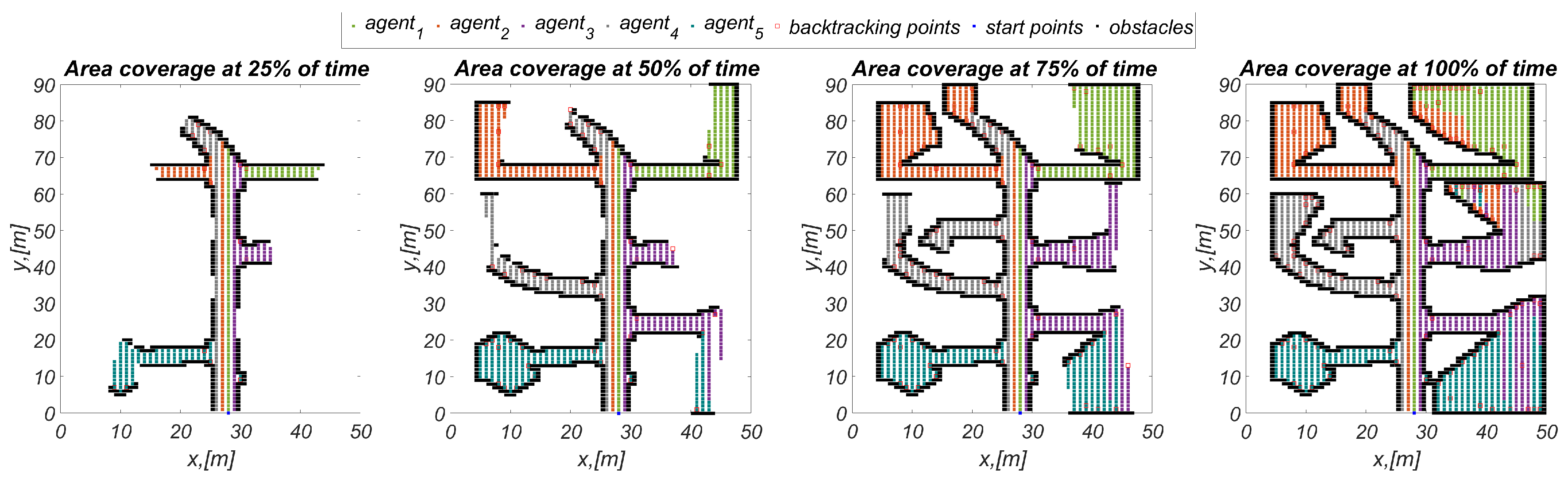
The area in the first scenario has a size of and it contains multiple branches. Figure 7 depicts the evolution of the explored area for , , , and of the time from left to right with a team of 5 agents. It can be observed from changing the BTP face colours that each agent uses its own BTP stack until it is empty, and then uses the BTP from the global BTP stack. As an example the in of the simulation execution time utilized its own local BTP (red squares); however, in of the simulation time and after completing the local BTP, it moves to the global BTPs which were discovered with another agents.
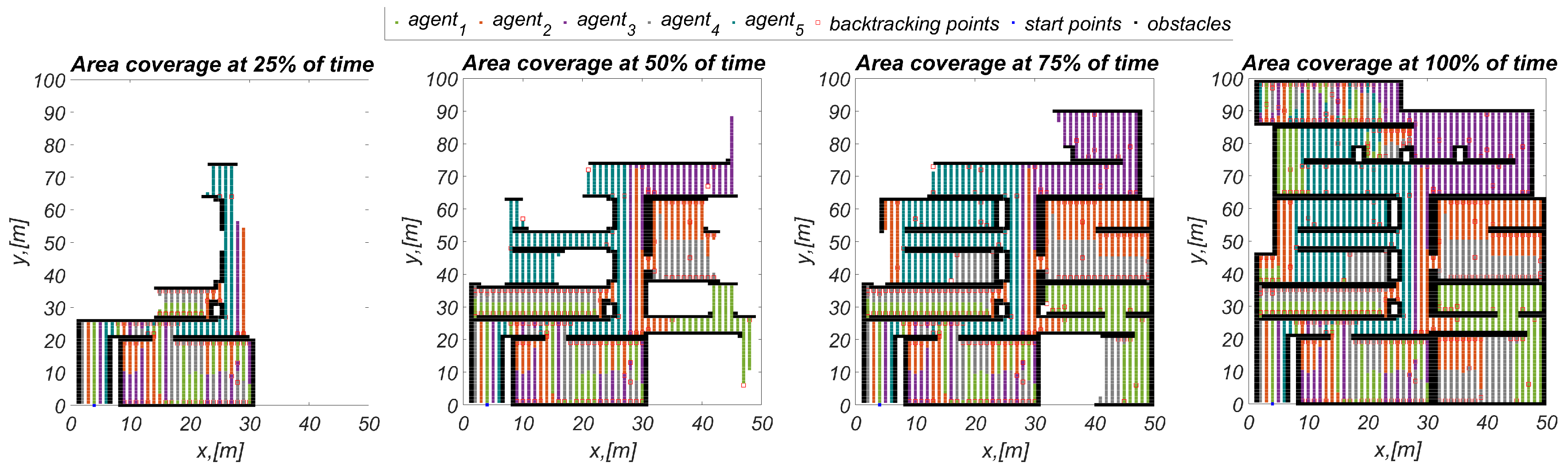
In the second case environment with size of with obstacles inside the exploration area is considered. Same as first case the exploration evolution over time with a team of five agents is shown in Figure 8. It can be seen that the proposed method results in the full coverage of the area.
Furthermore, in the third case, environment with size of , has higher complexity and number of branches is explored with team of five agents. Figure 9 depicts the exploration expansion over time.
The simulations for scenarios 1–3 demonstrated that the proposed method succeeds in completing coverage task. In order to analyze how well the work load is distributed between the agents the overall travelled path length of all agents in each scenario was analyzed. Figure 10 depicts the lengths of the coverage paths of the agents for each scenario. The proposed approach provides well balanced path lengths for each agent, as can be seen. Worth noting that the average path length for one agent in scenarios 1 and 2 represents a balanced workload for exploration areas of equivalent size, while the average path length for one agent in scenario 3 is bigger due to the larger size of the exploration area.
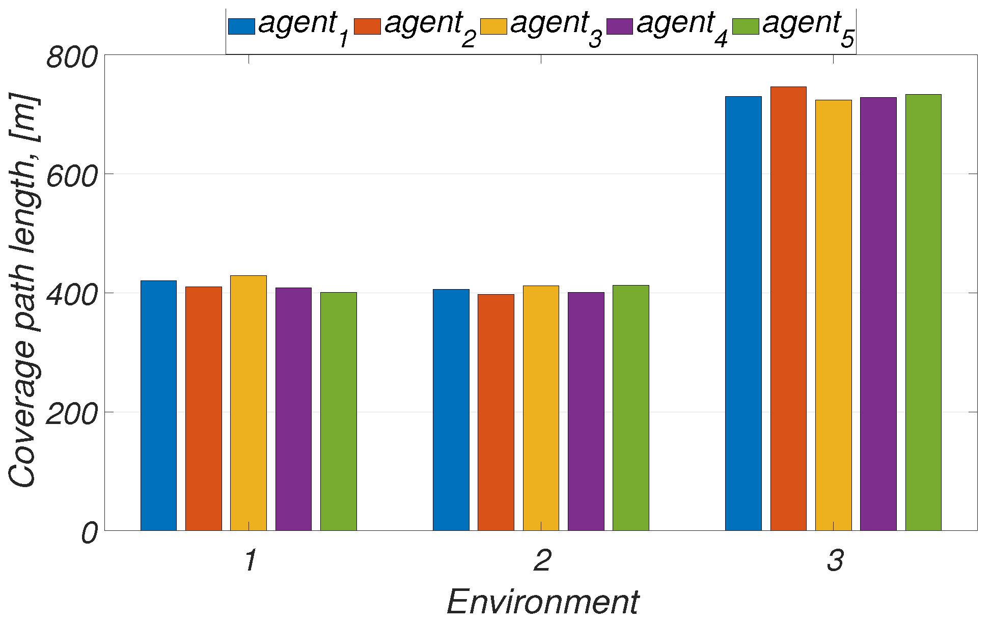
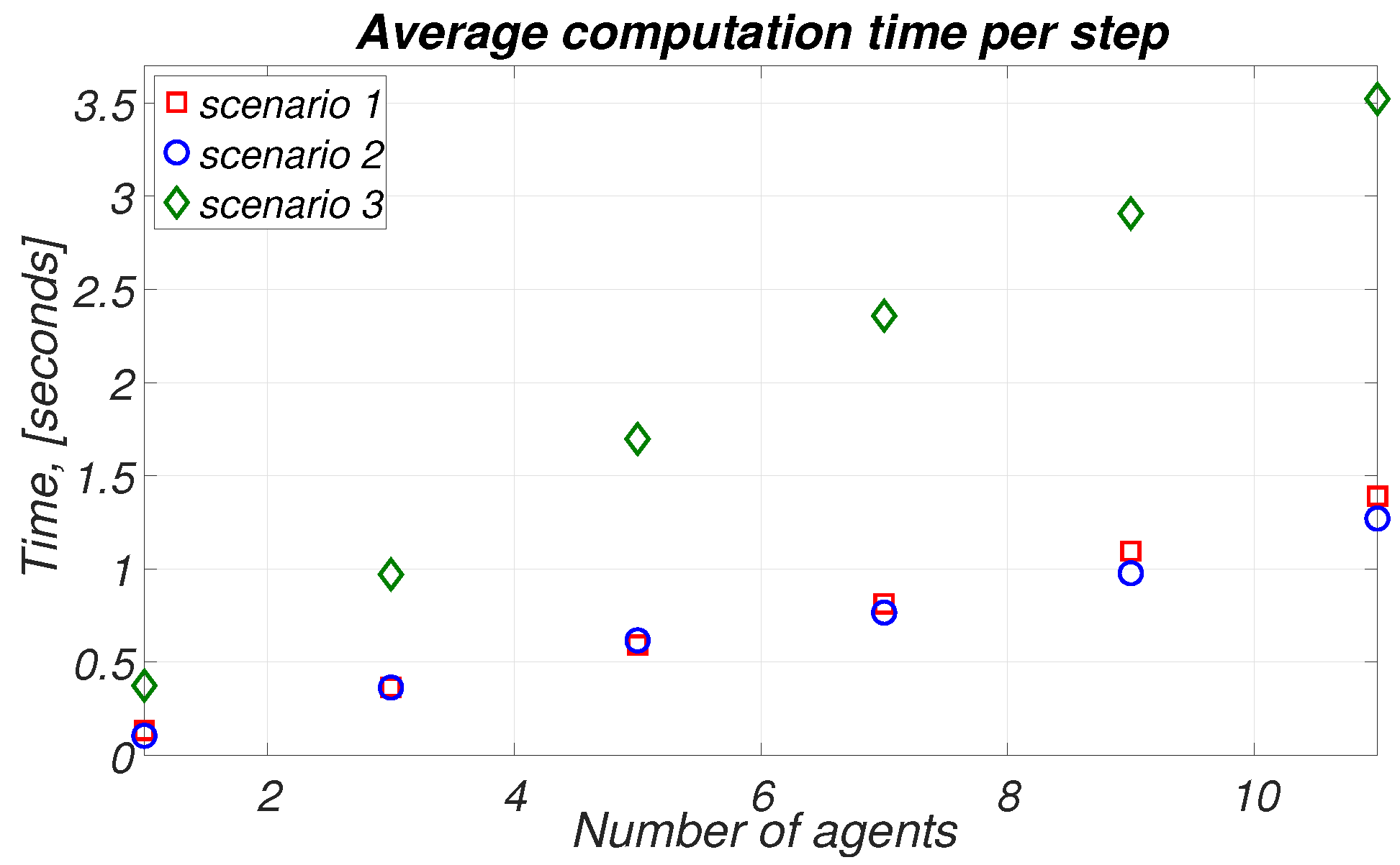
In order to assess how the exploration area size impacts on the algorithm performance with regards to the number of agents, the average time required to execute one step for one agent was calculated, as depicted in Figure 11. As one can see, the computation time for each scenario could be approximated linearly. Accordingly, the overall method is , which means that the rate of the computation time grows with the number of utilized agents. It can also be noted that the average computation time for exploration areas of the same sizes (Scenario 1 and 2) is around . This also means that, on average, the number of BTPs utilized to get trajectories by PRM planner in both scenarios is equal. For the scenario 3 with larger exploration area as compared to first two scenarios, agents discover more BTPs, thus path planning requires more computation time.
The further analysis will describe how the number of agents will influence the exploration process and the performance of the staying alive policy. In order to avoid data redundancy, the following results will only be presented for the first scenario.
In Figure 12 the relation between number of agents and the explored area over the time is presented. As expected, the larger team of agents results in less exploration time. However, it can be seen that the difference of exploration time between 9 and 11 agents is much less than difference of exploration time between 9 and 5. This shows that larger number of agents is not always necessary due to the size or structure of the environment; nonetheless, future study is required in order to find optimal number of agents.
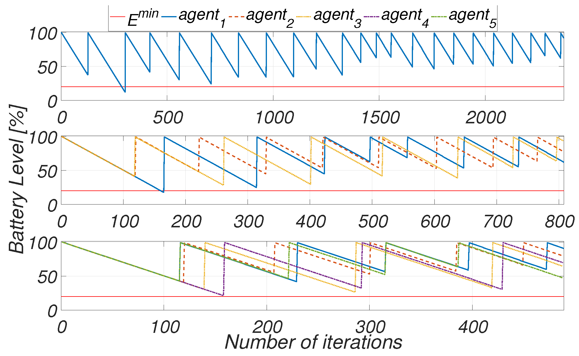
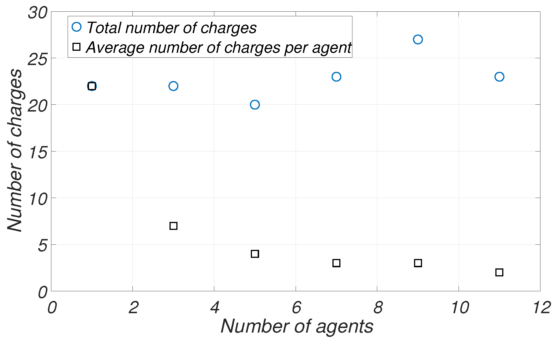
Figure 13 depicts the variation of agent’s charge level over the iteration process. The lower bound of the agent’s battery level is depicted as solid horizontal line in red colour. As it can be observed at the top and the middle images, the charge level goes below the stated bound. This means that, due to the large traveling distance from the charging point, the battery level dropped below . Thus, the introduced staying alive policy proved its viability in all conducted simulations by guaranteeing of agent loss. Further analysis revealed that the total number of charges per agent were reduced with a growth of the utilized agents.
In Figure 14 a comparison of the total number of charges required to explore the current simulation scenario, where for the case of 1 agent, the total and average number of charges are the same, is depicted. However, for larger teams, we observe fluctuations, e.g. in some cases the utilized team will have more charges than a single agent, but, on average, it will be more efficient and require less time for the entire exploration objective. Additionally, the average number of charges per agent varies, so, for example, in Figure 13 made five charges and made three charges.
Table 1 shows the summarized results of simulations for scenario 1.
In order to evaluate the performance of our approach with respect to other algorithms, two methods were chose [29]. One is the nonbacktracking multi-robot spanning tree coverage (NB-MSTC), an offline method that has proven to provide the smallest total length of the coverage paths and boustrophedon and backtracking mechanism (BoB) algorithm, which an online method developed for multi-robot systems. The criteria for comparison are the complete area coverage and the total length of the coverage paths. The workspace for evaluation was designed, as in Figure 9a in [29]. It has size of square cells and each cell has a size of and 13 obstacles, where each obstacle has cell width and a random length four to nine times the square cell.
The simulation results are presented in Figure 15, where the figure to the left is replotted Figure 9b from [29] that depicts the coverage path with four agents with NB-MSTC approach, while the figure to the right depicts the coverage path for the same number of agents with the proposed approach.
Table 2 summarizes the coverage paths for four agents by each method. As it can be seen, the NB-MSTC provides the shortest paths with the total coverage length of 617 m; however, as it can be seen from Figure 15, it does not provide a complete coverage and the workload between agents is not equally distributed. The BoB approach provides the total path length of 871 m, while keeping balanced work load distribution between agents. Unlike these two methods, the proposed algorithm created the total exploration path length of 716 m, while providing complete area coverage along with the balanced workload between agents.
Overall, the simulation results showed that the proposed approach works well in all simulated scenarios. Additionally, it outperforms NB-MSTC in area coverage and equally distributed work load among agents, and it outperforms BoB in terms of shorter total coverage path length of agents.
4.1. Discussions of the Design Choices
This article studied online multi-agent collaborative exploration and coverage of the unknown environment. Due to real-life challenges, such as search and rescue mission where the time of operation is important for situational assessments, this online approach selected and designed components of the presented algorithm.
The exploration method that is presented in Section 3.1 was selected according to conducted analysis of existing online exploration and coverage strategies. Among which, the Boustrophedon motion algorithm showed reasonable performance and capability for collaborative multi-agent work implementation in unknown environments.
The second method in Section 3.2 of the proposed algorithm was intentionally selected in order to bring it closer to the real life applications. Because, presently all platforms have limited operation time. This consideration allowed for us to implement the staying alive policy, which, according to conducted simulations, guarantees that all agents do not run out of energy within entire exploration and coverage mission.
Accordingly, the first two methods allow for conducting online exploration considering limited operation time. However, they cannot handle transitions when the agent reaches its blocked condition depicted at Figure 3 or runs out of charge. To overcome it and continue exploration (Figure 5), the path planner was used to generate collision free trajectories. Generally, for this, any path planner with such a capability can be used.
4.2. Design of Experiments
The transition from simulations to actual experiments will be done by the means of the Robot Operating System (ROS) [40], a framework for developing robotic applications, in which implementation of the designed algorithm together with robot control package will be implemented and tested. The assumptions that were taken in simulation, like robot dynamics, perfect localization, perfect sensor model, and communication, are the limitations that will be considered in planning the experiment. As a robotic platform, we selected turtlebot3, a standard ROS robot that provides full access to its on-board sensors for obtaining information about robot’s state and it can be remotely controlled from a laptop. The robot is equipped with 360 Laser Distance Sensor LDS-01 with maximum detection distance that is equal to 3500 mm. The lidar data will be processed in a way to reflect the sensing model that is used in simulation. The communication link between robots and laptop will be established while using WiFi connection. The Ubuntu based laptop will have ROS on-board and it will stand as a base station for controlling robots. The workspace will be designed when considering the turtlebot’s dimensions and, generally, will be smaller and less complicated than in the simulations. When considering its size and platform’s operating time of about 2 h, will be developed commands that will simulate low battery and full charge events for robot agents. Validation of the coverage and position tracking will be done while using motion capture system Vicon. During the experiment, all sensory information from the turtlebots’ and Vicon will be recorded by the means of ROS and processed afterwards. The obtained results from the experiments and simulations will be compared.
5. Conclusions
In this study, we introduced a novel online coverage approach for multi-agent systems in an unknown environment that can be used in inspection, search and rescue missions, and the exploration of the unknown areas of different complexitym and it considers deployment and coordination of multiple agents in close to real-life scenarios. The additional novelty of the proposed algorithm is that it couples the agent’s limited battery operation time with the path planner in order to guarantee a staying alive path planning for the multi-agent team. Moreover, a novel BTP point detection scheme for exploration task, while performing Boustrophedon motion, has been presented. The overall proposed online algorithm was successfully evaluated in simulations in complex environments by providing complete coverage of the exploration area and equally distributing the workload between agents. The overall provided path length of the proposed approach outperformed the BoB algorithm with 716 m against 871 m. Trajectories that were provided by the PRM planner were not always optimal and it requires more investigation towards local optimal path planning and remains to be part of future research. The influence of the exploration area size on the calculation time was demonstrated. This indicates that the larger exploration area, on average, has more BTPs, which, in turn, requires more trajectories to be calculated by the path planner. The implemented staying alive policy in all of the simulations guaranteed achieving a zero agent loss. The observed number of total charges required per agent for the simulated scenario is generally decreasing with a larger team, but there could be no guarantee that the total number of charges will be less than those for the one agent case. Part of the future research includes the enhancement and fusion of the presented staying alive policy by the path planning algorithm that is based on a real discharging model and the full experimental verification of the suggested scheme with mobile and aerial robots. Besides that, it is planned to investigate the feasibility of the agent in order to reach the end-point of the exploration area with a possibility to return safely to the starting point.
Author Contributions
Investigation, A.K.; Methodology, A.K. and S.S.M.; Supervision, G.N.; Validation, A.K.; Writing—original draft, A.K.; Writing—review and editing, A.K., S.S.M. and G.N. All authors have read and agreed to the published version of the manuscript.
Funding
This work has been partially funded by the European Unions Horizon 2020 Research and Innovation Programme under the Grant Agreement No. 375850 Robosol.
Conflicts of Interest
The authors declare no conflict of interest.
References
- Wasik, A.; Pereira, J.N.; Ventura, R.; Lima, P.U.; Martinoli, A. Graph-Based Distributed Control for Adaptive Multi-Robot Patrolling through Local Formation Transformation. In Proceedings of the 2016 IEEE/RSJ International Conference on Intelligent Robots and Systems (IROS), Daejeon, Korea, 9–14 October 2016. [Google Scholar]
- Yashoda, H.; Piumal, A.; Polgahapitiya, P.; Mubeen, M.; Muthugala, M.; Jayasekara, A. Design and Development of a Smart Wheelchair with Multiple Control Interfaces. In Proceedings of the 2018 Moratuwa Engineering Research Conference (MERCon), Moratuwa, Sri Lanka, 30 May–1 June 2018; pp. 324–329. [Google Scholar]
- Dautenhahn, K. Roles and functions of robots in human society: Implications from research in autism therapy. Robotica 2003, 21, 443–452. [Google Scholar] [CrossRef] [Green Version]
- Thrun, S.; Bennewitz, M.; Burgard, W.; Cremers, A.B.; Dellaert, F.; Fox, D.; Hahnel, D.; Rosenberg, C.; Roy, N.; Schulte, J.; et al. MINERVA: A second-generation museum tour-guide robot. In Proceedings of the 1999 IEEE International Conference on Robotics and Automation, Detroit, MI, USA, 10–15 May 1999; Volume 3. [Google Scholar]
- Cubber, G.D.; Doroftei, D.; Rudin, K.; Berns, K.; Serrano, D.; Sanchez, J.; Govindaraj, S.; Bedkowski, J.; Roda, R. Search and Rescue Robotics-From Theory to Practice; IntechOpen Limited: London, UK, 2017. [Google Scholar]
- Montambault, S.; Pouliot, N. Design and validation of a mobile robot for power line inspection and maintenance. In Proceedings of the 6th International Conference on Field and Service Robotics-FSR, Chamonix, France, 9–12 July 2007; Springer: Berlin/Heidelberg, Germany, 2007; Volume 42. [Google Scholar]
- Das, J.; Cross, G.; Qu, C.; Makineni, A.; Tokekar, P.; Mulgaonkar, Y.; Kumar, V. Devices, systems, and methods for automated monitoring enabling precision agriculture. In Proceedings of the 2015 IEEE International Conference on Automation Science and Engineering (CASE), Gothenburg, Sweden, 24–28 August 2015; pp. 462–469. [Google Scholar]
- Biswas, J.; Veloso, M. Depth camera based indoor mobile robot localization and navigation. In Proceedings of the 2012 IEEE International Conference on Robotics and Automation (ICRA), Saint Paul, MN, USA, 14–18 May 2012; pp. 1697–1702. [Google Scholar]
- Suarez, J.; Murphy, R.R. Using the Kinect for search and rescue robotics. In Proceedings of the 2012 IEEE International Symposium on Safety, Security, and Rescue Robotics (SSRR), College Station, TX, USA, 5–8 November 2012; pp. 1–2. [Google Scholar]
- Okura, F.; Ueda, Y.; Sato, T.; Yokoya, N. Teleoperation of mobile robots by generating augmented free-viewpoint images. In Proceedings of the 2013 IEEE/RSJ International Conference on Intelligent Robots and Systems (IROS), Tokyo, Japan, 3–7 November 2013; pp. 665–671. [Google Scholar]
- Pandey, A.; Pandey, S.; Parhi, D. Mobile robot navigation and obstacle avoidance techniques: A review. Int. Robot. Autom. J. 2017, 2, 00022. [Google Scholar] [CrossRef] [Green Version]
- Mansouri, S.S.; Kanellakis, C.; Kominiak, D.; Nikolakopoulos, G. Deploying MAVs for autonomous navigation in dark underground mine environments. Robot. Auton. Syst. 2020, 126, 103472. [Google Scholar] [CrossRef]
- Koval, A.; Kanellakis, C.; Vidmark, E.; Haluska, J.; Nikolakopoulos, G. A Subterranean Virtual Cave World for Gazebo based on the DARPA SubT Challenge. arXiv 2020, arXiv:2004.08452. [Google Scholar]
- Rodrigues de Campos, G.; Dimarogonas, D.V.; Seuret, A.; Johansson, K.H. Distributed control of compact formations for multi-robot swarms. IMA J. Math. Control Inf. 2017, 35, 805–835. [Google Scholar] [CrossRef]
- Mansouri, S.S.; Kanellakis, C.; Fresk, E.; Lindqvist, B.; Kominiak, D.; Koval, A.; Sopasakis, P.; Nikolakopoulos, G. Subterranean MAV Navigation based on Nonlinear MPC with Collision Avoidance Constraints. arXiv 2020, arXiv:2006.04227. [Google Scholar]
- Galceran, E.; Carreras, M. A survey on coverage path planning for robotics. Robot. Auton. Syst. 2013, 61, 1258–1276. [Google Scholar] [CrossRef] [Green Version]
- Khan, A.; Noreen, I.; Habib, Z. On Complete Coverage Path Planning Algorithms for Non-holonomic Mobile Robots: Survey and Challenges. J. Inf. Sci. Eng. 2017, 33, 101–121. [Google Scholar]
- Rekleitis, I.; New, A.P.; Rankin, E.S.; Choset, H. Efficient boustrophedon multi-robot coverage: An algorithmic approach. Ann. Math. Artif. Intell. 2008, 52, 109–142. [Google Scholar] [CrossRef] [Green Version]
- Zhou, P.; Wang, Z.; Li, Z.; Li, Y. Complete coverage path planning of mobile robot based on dynamic programming algorithm. In Proceedings of the 2nd International Conference on Electronic and Mechanical Engineering and Information Technology, Shenyang, China, 7 September 2012; pp. 1837–1841. [Google Scholar]
- Batsaikhan, D.; Janchiv, A.; Lee, S.G. Sensor-based incremental boustrophedon decomposition for coverage path planning of a mobile robot. In Intelligent Autonomous Systems 12; Springer: Berlin/Heidelberg, Germany, 2013; pp. 621–628. [Google Scholar]
- Bretl, T.; Hutchinson, S. Robust coverage by a mobile robot of a planar workspace. In Proceedings of the 2013 IEEE International Conference on Robotics and Automation (ICRA), Karlsruhe, Germany, 6–10 May 2013; pp. 4582–4587. [Google Scholar]
- Wang, Z.; Zhu, B. Coverage path planning for mobile robot based on genetic algorithm. In Proceedings of the 2014 IEEE Workshop on Electronics, Computer and Applications, Ottawa, ON, Canada, 8–9 May 2014; pp. 732–735. [Google Scholar]
- Yu, X.; Hung, J.Y. Coverage path planning based on a multiple sweep line decomposition. In Proceedings of the IECON 2015-41st Annual Conference of the IEEE Industrial Electronics Society, Yokohama, Japan, 9–12 November 2015; pp. 004052–004058. [Google Scholar]
- Broderick, J.; Tilbury, D.; Atkins, E. Energy usage for UGVs executing coverage tasks. In Unmanned Systems Technology XIV; International Society for Optics and Photonics: Bellingham, WA, USA, 2012; Volume 8387, p. 83871A. [Google Scholar]
- Broderick, J.; Tilbury, D.; Atkins, E. Maximizing coverage for mobile robots while conserving energy. In Proceedings of the ASME 2012 International Design Engineering Technical Conferences and Computers and Information in Engineering Conference, Chicago, IL, USA, 12–15 August 2012; American Society of Mechanical Engineers: New York, NY, USA, 2012; pp. 791–798. [Google Scholar]
- Strimel, G.P.; Veloso, M.M. Coverage planning with finite resources. In Proceedings of the 2014 IEEE/RSJ International Conference on Intelligent Robots and Systems, Chicago, IL, USA, 14–18 September 2014; pp. 2950–2956. [Google Scholar]
- Viet, H.H.; Choi, S.; Chung, T. An online complete coverage approach for a team of robots in unknown environments. In Proceedings of the 2013 13th International Conference on Control, Automation and Systems (ICCAS), Gwangju, Korea, 20–23 October 2013; pp. 929–934. [Google Scholar]
- Viet, H.H.; Dang, V.H.; Laskar, M.N.U.; Chung, T. BA*: An online complete coverage algorithm for cleaning robots. Appl. Intell. 2013, 39, 217–235. [Google Scholar] [CrossRef]
- Viet, H.H.; Dang, V.H.; Choi, S.; Chung, T.C. BoB: An online coverage approach for multi-robot systems. Appl. Intell. 2015, 42, 157–173. [Google Scholar] [CrossRef]
- Choi, S.; Lee, S.; Viet, H.H.; Chung, T. B-Theta*: An Efficient Online Coverage Algorithm for Autonomous Cleaning Robots. J. Intell. Robot. Syst. 2017, 87, 265–290. [Google Scholar] [CrossRef]
- Masehian, E.; Jannati, M.; Hekmatfar, T. Cooperative mapping of unknown environments by multiple heterogeneous mobile robots with limited sensing. Robot. Auton. Syst. 2017, 87, 188–218. [Google Scholar] [CrossRef]
- Rekleitis, I.; New, A.P.; Choset, H. Distributed coverage of unknown/unstructured environments by mobile sensor networks. In Multi-Robot Systems. From Swarms to Intelligent Automata Volume III; Springer: Berlin/Heidelberg, Germany, 2005; pp. 145–155. [Google Scholar]
- Kong, C.S.; Peng, N.A.; Rekleitis, I. Distributed coverage with multi-robot system. In Proceedings of the 2006 IEEE International Conference on Robotics and Automation (ICRA 2006), Orlando, FL, USA, 15–19 May 2006; pp. 2423–2429. [Google Scholar]
- West, D.B. Introduction to Graph Theory; Prentice Hall: Upper Saddle River, NJ, USA, 2001; Volume 2. [Google Scholar]
- Balampanis, F.; Maza, I.; Ollero, A. Area partition for coastal regions with multiple UAS. J. Intell. Robot. Syst. 2017, 88, 751–766. [Google Scholar] [CrossRef]
- Khan, A.; Noreen, I.; Ryu, H.; Doh, N.L.; Habib, Z. Online complete coverage path planning using two-way proximity search. Intell. Serv. Robot. 2017, 10, 229–240. [Google Scholar] [CrossRef]
- Mansouri, S.S.; Karvelis, P.; Georgoulas, G.; Nikolakopoulos, G. Remaining useful battery life prediction for UAVs based on machine learning. IFAC-PapersOnLine 2017, 50, 4727–4732. [Google Scholar] [CrossRef]
- Wei, H.; Wang, B.; Wang, Y.; Shao, Z.; Chan, K.C. Staying-alive path planning with energy optimization for mobile robots. Expert Syst. Appl. 2012, 39, 3559–3571. [Google Scholar] [CrossRef]
- Svestka, P.; Latombe, J.; Overmars Kavraki, L. Probabilistic roadmaps for path planning in high-dimensional configuration spaces. IEEE Trans. Robot. Autom. 1996, 12, 566–580. [Google Scholar]
- Quigley, M.; Conley, K.; Gerkey, B.; Faust, J.; Foote, T.; Leibs, J.; Wheeler, R.; Ng, A.Y. ROS: An open-source Robot Operating System. In Proceedings of the ICRA Workshop on Open Source Software, Kobe, Japan, 12–17 May 2009; Volume 3, p. 5. [Google Scholar]
Figure 1.
General scheme of the proposed approach, where q denotes the agents and their positions, denotes the free area, denotes the backtracking points, denotes the obstacles, and the undiscovered area is presented in a white colour.
Figure 1.
General scheme of the proposed approach, where q denotes the agents and their positions, denotes the free area, denotes the backtracking points, denotes the obstacles, and the undiscovered area is presented in a white colour.

Figure 2.
The conditions of backtracking point (BTP) detection.

Figure 3.
The blocked conditions for the agent with forward motion. Green arrow depicts motion direction, white tiles denote agent’s discovered path, grey tiles denote free space. The left image describes the case when the agent is blocked by obstacles (black tiles), the middle image depicts the case when the agent is blocked with obstacles on the left and the neighbouring areas are covered by other agents. The image on the right depicts the case when all neighbouring regions were discovered by other agents.

Figure 4.
Example of the Probabilistic Roadmap (PRM) planner, applied on a time instant of the explored area, where free (discovered) space is in white, undiscovered area is in grey, obstacles are in black, and the generated path is in orange. In this Figure, the graph with all of the PRM based potential paths is indicated by blue.

Figure 5.
Example of cases for collision free path generation by PRM planner. (a)—corresponds to the blocked case, where the further exploration directions are shown by dashed orange arrows and (b)—is low battery level case where the path to the charging point is indicated by dotted green arrow. Where, BM is shown in blue colour. Green circle corresponds to the start point or and brown circle corresponds to finish of the BM, e.g., (blocked position). Red squares correspond to detected BTPs (). The discovered area is depicted in white, unknown area is depicted in grey, and obstacles are in black.

Figure 6.
The entire system design for multi-agent cooperative exploration and coverage.

Figure 7.
Scenario 1. Area discovered with five agents, launched from the same location. The black areas are obstacles, while the red squares are backtracking points (BTPs).
Figure 7.
Scenario 1. Area discovered with five agents, launched from the same location. The black areas are obstacles, while the red squares are backtracking points (BTPs).

Figure 8.
Scenario 2. Area discovered with five agents, launched from the same location. The black areas are obstacles, while the red squares are BTPs.
Figure 8.
Scenario 2. Area discovered with five agents, launched from the same location. The black areas are obstacles, while the red squares are BTPs.

Figure 9.
Scenario 3. Area discovered with five agents, launched from the same location. The black areas are obstacles, while the red squares are backtracking points (BTPs).
Figure 9.
Scenario 3. Area discovered with five agents, launched from the same location. The black areas are obstacles, while the red squares are backtracking points (BTPs).

Figure 10.
The length of coverage paths per agent in a team of five agents for three simulated scenarios, respectively.
Figure 10.
The length of coverage paths per agent in a team of five agents for three simulated scenarios, respectively.

Figure 11.
Average computation time of the proposed Algorithm 4 per one step for teams of agents for three scenarios.
Figure 11.
Average computation time of the proposed Algorithm 4 per one step for teams of agents for three scenarios.

Figure 12.
Explored area with teams of agents.

Figure 13.
Charge level time evolution for one, three, and five agents.

Figure 14.
The total and average number of charges for teams of agents.

Figure 15.
The coverage path of four agents. NB-MSTC to the left, proposed approach to the right.


Table 1.
Simulation results of area exploration with proposed algorithm.
| Environment | Size of Environment, | Number of Agents | Total Number of Charges for One Agent | Average Computation Time for 1 Step, s | Number of Iterations |
|---|---|---|---|---|---|
| 1 | 22 | 0.13 | 2365 | ||
| 3 | 7 | 0.36 | 804 | ||
| Scenario 1 | 2068 | 5 | 5 | 0.59 | 491 |
| 7 | 3 | 0.81 | 363 | ||
| 9 | 3 | 1.09 | 314 | ||
| 11 | 2 | 1.39 | 259 |
Table 2.
The coverage path length achieved by NB-MSTC, backtracking mechanism (BoB), and proposed algorithm.
Table 2.
The coverage path length achieved by NB-MSTC, backtracking mechanism (BoB), and proposed algorithm.
| Algorithm | Coverage Path Length by Agent, [m] | |||
|---|---|---|---|---|
| 1 | 2 | 3 | 4 | |
| NB-MSTC | 172 | 400 | 24 | 21 |
| BoB | 199 | 215 | 224 | 233 |
| Proposed approach | 171 | 187 | 178 | 180 |
Publisher’s Note: MDPI stays neutral with regard to jurisdictional claims in published maps and institutional affiliations. |
© 2020 by the authors. Licensee MDPI, Basel, Switzerland. This article is an open access article distributed under the terms and conditions of the Creative Commons Attribution (CC BY) license (http://creativecommons.org/licenses/by/4.0/).
Share and Cite
MDPI and ACS Style
Koval, A.; Sharif Mansouri, S.; Nikolakopoulos, G. Multi-Agent Collaborative Path Planning Based on Staying Alive Policy. Robotics 2020, 9, 101. https://0-doi-org.brum.beds.ac.uk/10.3390/robotics9040101
AMA Style
Koval A, Sharif Mansouri S, Nikolakopoulos G. Multi-Agent Collaborative Path Planning Based on Staying Alive Policy. Robotics. 2020; 9(4):101. https://0-doi-org.brum.beds.ac.uk/10.3390/robotics9040101
Chicago/Turabian StyleKoval, Anton, Sina Sharif Mansouri, and George Nikolakopoulos. 2020. "Multi-Agent Collaborative Path Planning Based on Staying Alive Policy" Robotics 9, no. 4: 101. https://0-doi-org.brum.beds.ac.uk/10.3390/robotics9040101
Note that from the first issue of 2016, this journal uses article numbers instead of page numbers. See further details here.