1. Introduction
This study is part of the Autonomous Robot Evolution (
https://www.york.ac.uk/robot-lab/are/) project that is concerned with robots that can reproduce and evolve in the real world [
1,
2]. The long-term objective is to enable the evolution of an entire autonomous robotic ecosystem, where robots live and work for long periods in challenging and dynamic environments without the need for direct human oversight. The envisioned system has two features which, when combined, make it special and very challenging: it concerns the evolution of physical robots—not only simulated ones—and it is not limited to the evolution of robot controllers (brains), but also concerns the evolution of the robots’ morphologies (body plans).
The construction of a real-world robot is much more time- and resource-consuming than the construction of a digital robot, a piece of code that represents a robot in simulation. The difference can be huge; for instance making a robot in a simulator may take less than a second consuming only small amounts of energy, CPU power and memory, while building a real robot can easily take many hours and consume significant energy, raw materials and components. This means that each evolutionary trial should be considered carefully and should not be wasted. Secondly, further to the physical phenotype challenge, we have the fabrication challenge. That is, new robots do not just miraculously materialise, but need to be fabricated, and the fabrication process implies its own implementation-specific constraints. In an autonomous robot evolution system, automated fabrication is necessary, without human assistance. For example, the ARE project uses a 3D-printer, an ‘organ bank’ of prefabricated (non-printable) components and a robot arm that assembles all body parts to form a new robot (the phenotype) according to the given specification (the genotype). The operation of such an autonomous fabrication system is constrained by several practical details, e.g., the limitations of the 3D-printer, the shapes, sizes and interfaces of the prefabricated ‘organs’, and the position, size and geometry of the assembly arm. Thus, the essence of the fabrication challenge is that a robot needs to be not only conceivable but also manufacturable.
A potential solution for both challenges discussed above is the screening of robotic genotypes. To consider what this means, note that reproduction consists of two principal steps. Given two parent robots, the first step is to apply the crossover operator to their genotypes and produce a new genotype that encodes the offspring. This is a fully digital operation, hence relatively cheap. The expensive step is the second one, when the genotype-phenotype mapping is executed, in other words, when the physical robot ‘child’ is constructed. The idea of screening is to make the second step conditional by inspecting the new genotype, estimating the manufacturability of the corresponding robot and cancelling the fabrication of the phenotype if the outcome is negative. Obviously, manufacturability is not the only feature screening can consider. Specifically, it may be possible to rate the expected viability of a new robot, for instance, to check if it could move, or to estimate the (range of) its fitness value. Thus, in general, screening can take morphological properties, like manufacturability, as well as behavioural properties, like viability, into account.
Technically speaking, screening amounts to introducing constraints and a notion of feasibility regarding the search space. In the classic evolutionary algorithms (EA) literature, constrained optimisation problems can be handled in two different ways, (1) allowing infeasible solutions during the search, but using a penalty function, or (2) not allowing infeasible solutions and evolving in a feasible space. The first option is not applicable in this case because a solution that is not feasible means a robot that is not manufacturable.
The second option requires that evolution takes place in the feasible part of the search space. An essential prerequisite to this end is that the initial population consists of manufacturable robots. Furthermore, the initial population should be diverse, as this increases the probability of finding the best robots for the given environment and task. The main objective of this paper is to develop a method to generate both feasible and diverse initial populations.
The feasibility of physically fabricating evolved robots has been demonstrated by a handful of studies [
3,
4,
5,
6,
7]. However, the robots in these studies are very simple; they have actuators to move, but they lack sensors to perceive the environment. In addition, constructing new robots is a very tedious process that relies much on human assistance. Only Brodbeck et al. [
4] achieved the autonomous fabrication of robots at the cost of extremely simplifying the robot designs and the fabrication process: their robots consist of three to five cubes stacked upon each other and glued together, driven by an external computer. The ARE project works with complex autonomous robots with several different components, including a CPU, actuators, sensors and 3D printed complex shapes. The challenges of autonomous fabrication of robots in ARE have been highlighted in [
2,
8,
9] where the Robot Fabricator (the machine that fabricates robots) imposes different constraints in 3D printing and autonomous assembly.
This paper has two main contributions. First, a method to generate a diverse set of manufacturable and viable robots. Second, an assessment of the robots this method delivers from two perspectives, (a) their learning potential and (b) their evolutionary potential. For (a), a controller is learned for each body plan in the bootstrap population. For (b), we use them as the initial population for an artificial evolutionary process. For this investigation, we consider three environments concerning navigation.
The approach and experimental workflow is summarised in
Section 3. Firstly, a novelty search algorithm is used to produce a large and diverse pool of body plans. Three body plan descriptors (vector describing specific features of the robots) are compared to find the most efficient way to explore the search space. Then, a population of robots is selected from this pool. Four selection processes are compared based on their capacity to produce the most diverse population. This population is evaluated in a maze navigation task with randomly-sampled controllers and learned controllers for each body plan in the population. Finally, the population of body plans is used to bootstrap an evolutionary process. To assess the benefit of using this bootstrap population, the same experiments are also conducted with a randomly sampled population.
The specific research questions investigated are the following:
What is the best combination of descriptor and selection method to maximise the diversity of body plans in the bootstrap population?
What are the benefits of evolving a diverse bootstrap population over simply randomly sampling from the space of body plans?
Are the robots formed by the bootstrap population more capable of solving a navigation task than a randomly sampled population (when combined with method(s) to learn a controller)?
The key results from this paper are that the use of bootstrap population is beneficial for (a) the generation of a population of robots diverse enough to produce robots capable of solving simple environments; and (b) reduce the number of evaluations required to converge to the solution when evolution is used. Most importantly, this method aids to overcome the challenges of finding body plans in a difficult landscape constrained by the limitations of autonomous robot fabrication.
This paper extends the results from [
9] by investigating additional alternative descriptors to determine which descriptor is most efficient. This paper has the following novel additional contributions.
An investigation was carried out on various selection methods to determine which robots were selected to form an initialised population.
The behavioural potential in each evolved robot of the population was evaluated by using a controller learning mechanism in three different environments.
The body plans and controllers were evolved simultaneously, starting with a bootstrapped population and a random population in three different environments.
2. Related Work
As outlined above, the idea of evolving the body plans for “virtual organisms” or “robotic lifeforms” has been around for decades, but existing work is limited to conducting evolution in computer simulations. The long-term vision regarding physically embodied artificial evolutionary systems has been first outlined in 2012 by Eiben et al. who described the main concepts and discussed the related promises and challenges, but provided no specific guidelines for actual implementations [
10]. Such guidelines were given in [
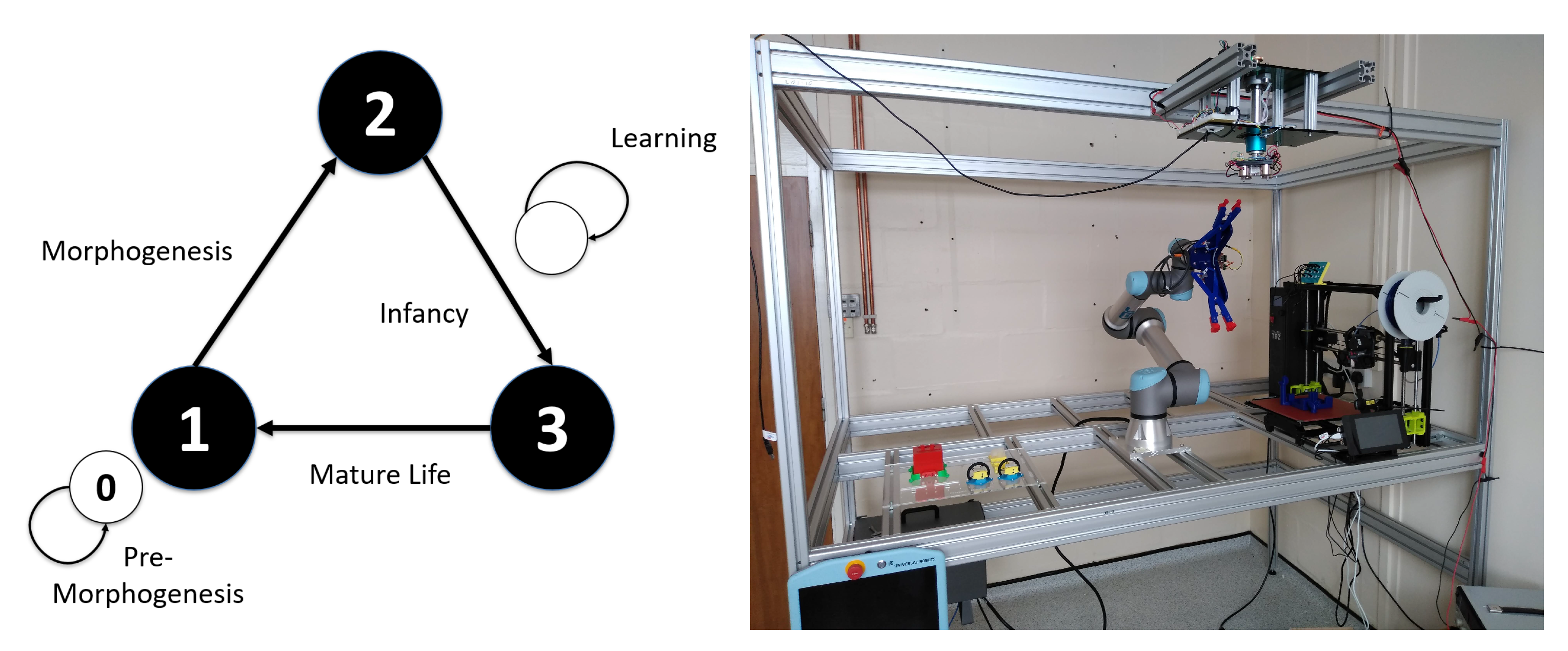
11] that presented a generic system architecture, named the Triangle of Life (ToL) for “robots that evolve in real-time and real-space”. The Triangle of Life framework is illustrated on the left-hand side of
Figure 1. It consists of three principal stages: morphogenesis, infancy and mature life. Consequently, a tangible implementation consists of three main system components: the Robot Fabricator, the Training Facility and the arena. The Robot Fabricator is where new robots are created. The Training Facility hosts a learning environment for ‘infant’ robots so they can learn to control their—possibly unique—body to acquire basic skills (e.g., locomotion, object manipulation) and to perform more complex tasks. If a robot achieves a satisfactory level of performance, it is declared a fertile adult and enters the arena (which represents the world where the robots must survive and perform user-defined tasks) and is considered a viable candidate for parenthood.
The autonomous robot fabrication in the Robot Fabricator has many challenges. It is easy to see why this is an important issue if we are to evolve physical robots: the resources are much more limited than in ‘simple’ computer simulations. Minimising resources is important because constructing a robot is expensive and even though the initial population is random, one should not waste resources, and should also make sure that the robots therein are individually transferable to reality and the population as a whole is transferable. The transferability of an individual robot can be defined through morphological or behavioural properties [
12]. Regarding body plans, the phenotype is required to be manufacturable.
This study is directly linked to the reality gap issue widely studied in evolutionary robotics (ER). The manufacturability constraints define robots that are transferable to reality. Most of the work in the literature on crossing the reality gap in ER addresses the behaviour of the robots. Different approaches have been proposed in literature, from (1) optimising the simulator to get closer to reality [
13,
14] or (2) simplifying the simulator to target the most important aspects of the task, thus narrowing the gap [
15] or (3) producing a large list of diverse behaviours and choosing the suitable behaviour according to the current situation [
16]. The closest approach to the present study is the transferability approach described in [
12]. This approach aims at finding measures to assess the similarities/differences between a controller running on a simulated robot and its physical counterpart. In this study, manufacturability is considered to be analogous to transferability, but applied to body plan designs. In terms of considering manufacturability of physical robots, one other approach is worthy of mention: recent work by Kriegman et al. [
6] describes a pipeline for creating living robots made from cells using an evolutionary process. Designs created by simulated evolution are first passed through a robustness filter which filters out evolved designs with behaviours that are not robust to noise, and then through a build filter [
6] which removes designs that are not suitable for the current build method or unlikely to scale to future tasks. Surviving designs are then hand built. A significant difference to the method proposed in this paper is that the filters are applied post-evolution and are not accounted for in any way during the evolutionary process.
In this paper, a new method for population initialisation of diverse and manufacturable robots is proposed. The objective of population initialisation in EAs is to provide an initial guess of solutions, and then this population will be iteratively improved over time. However, recent studies have shown that a good selection of the initial population can increase the probability of finding the global optima and decrease the time it takes to find it [
17]. Different strategies have been proposed in the literature with different results, and a survey of this literature can be found in [
18]. Nonetheless, to our knowledge, no strategies of population initialisation of robots that can be autonomously constructed have been explored in ER.
3. Experimental Framework
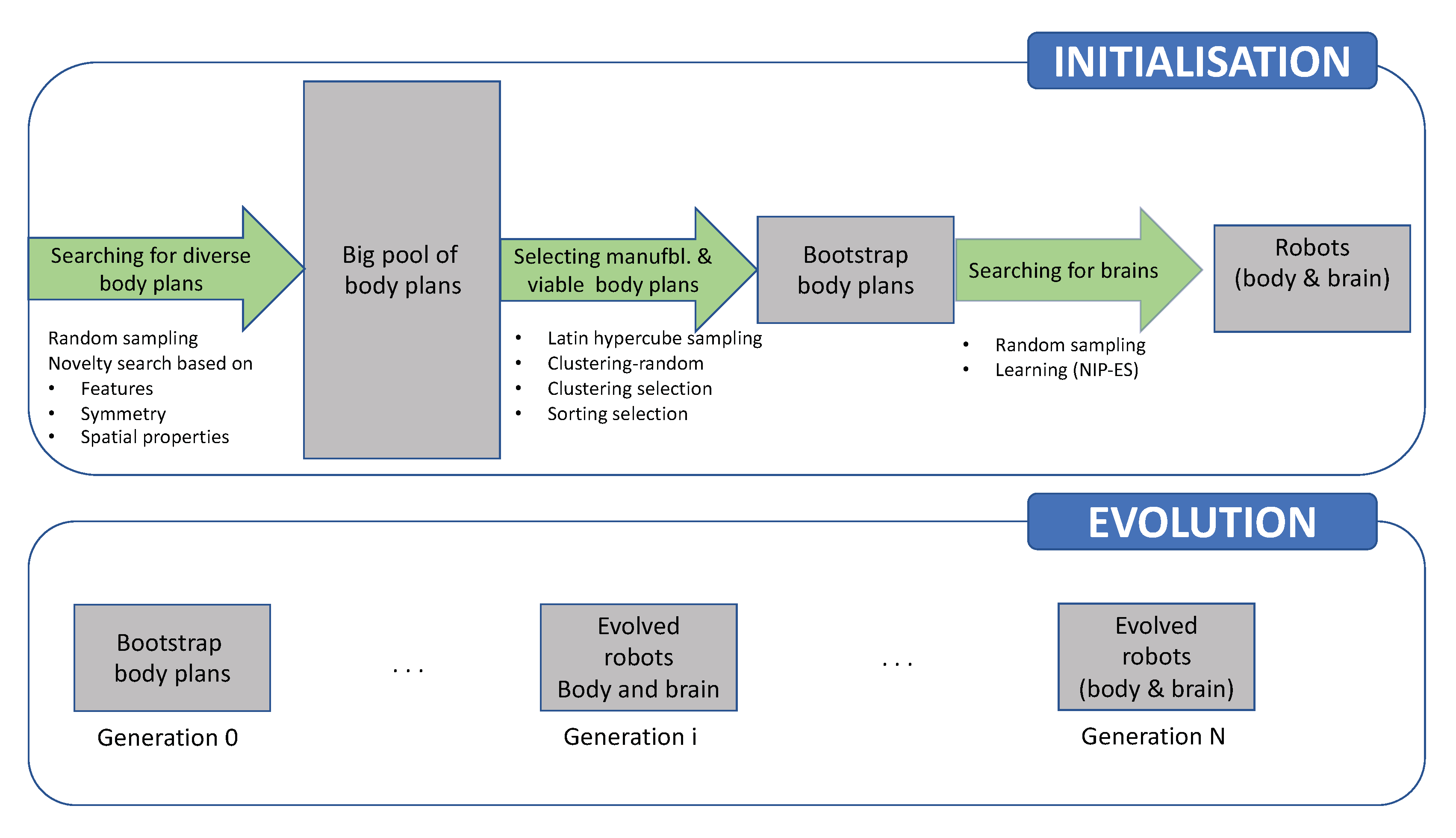
The experimental framework followed for this paper is shown in
Figure 2. Firstly, a large pool of diverse robots is evolved. Then, from this pool, a smaller subset of robots is selected as initial population, referred to as ‘bootstrap population’ in this paper. Finally, the capability of the body plans to solve a navigation task is measured with randomly-sampled controllers and learned controllers. In addition, the bootstrap population is tested with an experiment where the body plans and the controllers are further evolved to solve a navigation task.
3.1. Generation of a Large List of Diverse Body Plans
The main objective of this stage is to generate a large list of diverse robots that are also manufacturable. Therefore, one of the goals of this section is to identify the body plan descriptor that maximises diversity when the robots are evolved.
3.1.1. Body Plan Generation
The body plan generation used in this paper is a variation of the one introduced in [
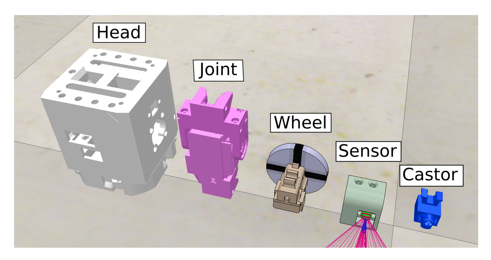
9]. The robots have two types of components: skeleton and organs. The skeleton is the 3D-printable structure that holds the robot together. Organs are the active or passive pre-fabricated components. The organs used in this paper are the head, joint, wheel, sensor and castor organs all shown in
Figure 3 and described next.
The head organ takes the role of receiving signals from the sensors and sending signals to the actuators (and includes the power source).
The joint organ is an actuator which takes frequency as an input and outputs the position of the actuator in the interval from −90 to 90 degrees.
The wheel organ is a rotational actuator which takes velocity as an input.
The sensor organ can output two different signals. The first signal is distance to the closest obstacle. The second signal is binary where the signal is 1 if the beacon is detected, or 0 if the beacon is not detected and it might be occluded by an obstacle.
The castor organ is a passive component which reduces the friction of the robot with the floor.
The body plans are encoded in a Compositional Pattern Producing Network (CPPN) first introduced by Stanley [
19], as it has been demonstrated that with this encoding it is possible to evolve complex patterns. The structure of the CPPN has 4 inputs and 6 outputs. The four inputs define the position of a cell in a 3D matrix with size 13 × 13 × 13 mm, where the first three inputs are the coordinates x, y and z, and the last input is the distance r from the centre of the cell. The six outputs define the properties of each cell in the 3D matrix. The first five outputs are binary and they represent the absence or presence of a specific type of voxel. There are five types of voxels: skeleton, wheel, sensor, joint and castor. The last output represents the rotation of a specific component around the normal of the surface of the skeleton.
The genotype to phenotype decoder operates as follows:
Firstly a single layer skeleton ’seed’ is generated around the head organ. After this, the skeleton output is queried for the entire 3D matrix. This will generate the plastic connecting all the organs. Only one region of skeleton is allowed per body plan, where a region is a cluster of inter-connecting skeleton voxels. The biggest region of skeleton is preserved and any regions unconnected to the ’seed’ are removed.
Then, the CPPN is queried to determine wheel, sensor, joint and castor outputs, generating multiple regions for each type. An organ is generated in each intersecting area between the organ region and the skeleton surface. This ensures that all the components are connected to the surface of the skeleton. Only one component is generated in each region regardless of the size of the intersecting area.
Two relative rotations of the organs are given by the normal of the skeleton surface. The third rotation around the relative axis of the organ is given by the last output of the CPPN.
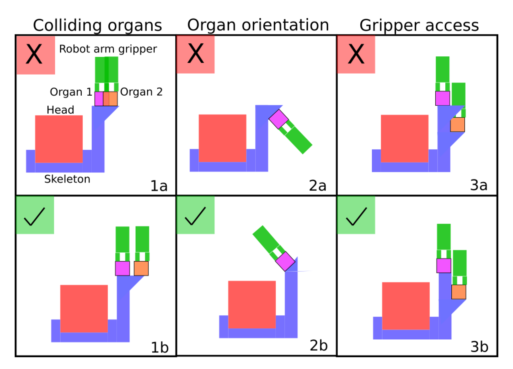
As mentioned in the introduction, the Robot Fabricator, shown in
Figure 1, imposes various constraints on the body plans that can be manufactured. These constraints are listed below and shown in
Figure 4:
With these constraints in mind, if one or more organs violate at least one of these constraints, they are removed from the final body plan.
Some examples of body plans evolved can be found in the video in [
20]. A video of the Robot Fabricator assembling a robot can be found in [
21].
3.1.2. Body Plan Descriptors
The aim of the body plan generation experiments is to generate a large diverse list of robots. For this, the novelty search algorithm is used. The novelty search algorithm [
22] replaces the traditional fitness function with one which rewards novelty. Novelty is measured by comparing a descriptor vector (which describes the body plan represented by an individual) with the descriptors of both the current population and those maintained in an archive produced by the same algorithm and described below (more details in
Appendix A):. In this paper we extend the work in [
9] where body plans were evolved for a single descriptor. For this paper three different descriptors are compared: the
feature descriptor,
symmetry descriptor and the
spatial descriptor. These descriptors are described next.
Feature Descriptor
The objective of this descriptor is to capture the features of a body plan with a low number of traits. In this case the descriptor, shown in Equation (
1), contains 8 traits:
The width, depth and height traits describe the volume of the robot.
The number of voxels represents the voxels used for the skeleton in the body plan.
The number of
wheels,
sensors,
joints and
castors traits represent the final number of these components in the body plan
Symmetry Descriptor
For the
symmetry descriptor, Equation (
2), the body plan is divided in 8 quadrants which follows the coordinate system, where the centre of this coordinate system is in the middle of the 3D matrix. Then, each trait in the vector counts the number of
voxels,
wheels,
sensors,
joints and
castors in each of the 8 quadrants.
Spatial Descriptor
The
spatial descriptor, Equation (
3), is the largest, and it encodes the content of each cell in the 3D matrix of the final body plan after generation. Each cell could have one of 6 different values: empty cell, skeleton or an organ type (wheel, sensor, joint or castor).
3.1.3. Experiments and Results
The main goal of the experiments in this section is to compare the different body plan descriptors introduced in the previous section in order to identify the descriptor that provides the most diverse set of body plans. For this, qualitative and quantitative results are shown. A total of 30,000 robots were produced for random sampling and for each body plan descriptor. A total of 20 replicates or repetitions are shown in these results.
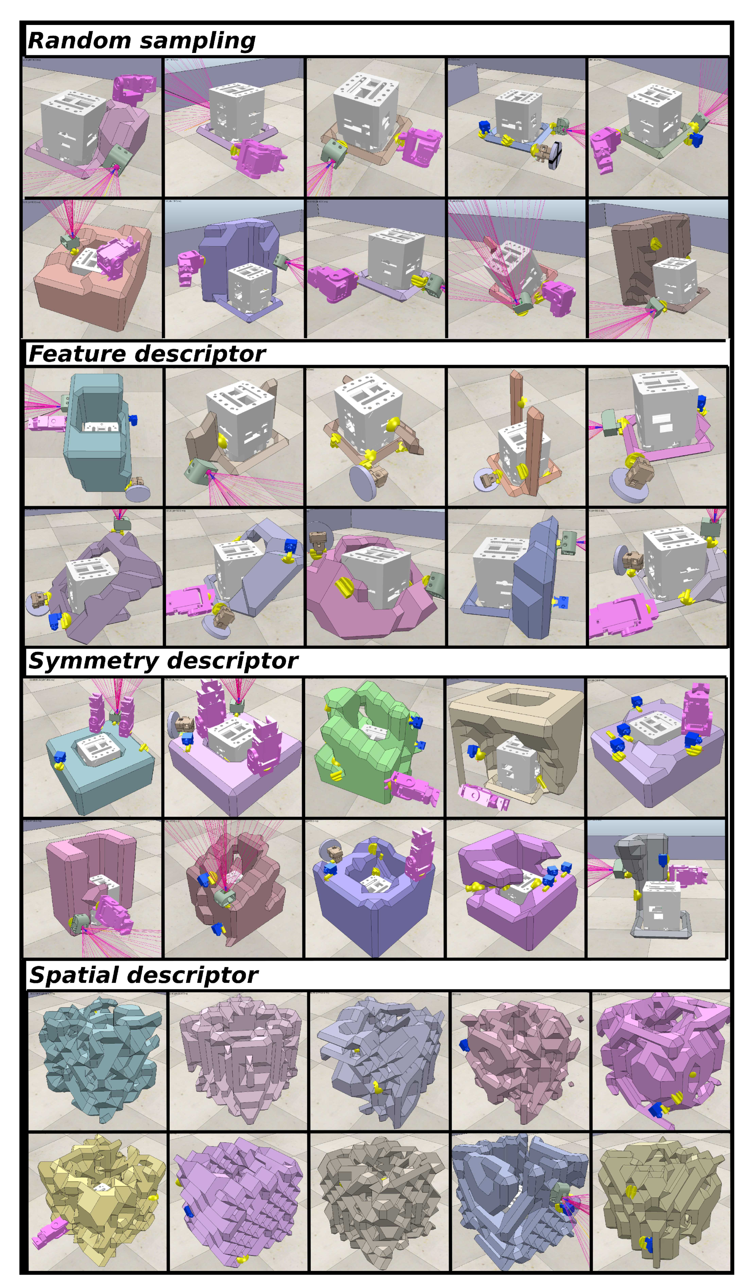
Figure 5 shows some examples of robots produced with
random sampling and evolved with each descriptor. The robots produced with
random sampling have simple skeletons (basic shapes) with a low number of organs. The random generation of CPPNs is not capable of creating patterns that create complex skeletons and robots with a high number of organs. Robots evolved with the
feature descriptor have the highest number of organs, but the skeletons are simple. Since half of the attributes of this descriptor measure the number of organs, the body plans are evolved with more organs. Robots evolved with the
symmetry descriptor have a higher number of organs with more complex skeletons. Robots evolved with the
spatial descriptor have the most complex skeletons with the lowest number of organs. This is because the number of skeleton-related traits outweighs the traits for organs in this descriptor.
As for quantitative results, the total number of robots with given number of organs is shown in
Table 1. The
feature descriptor generates the highest number of robots with different numbers of organs. The
spatial descriptor generates the list of robots with the lowest number of organs. This means that the
feature descriptor will have a greater probability of producing robots with the necessary organs to solve the given task.
The mean sparseness for each descriptor is shown in
Table 2 and measured using Equation (
A1). Unsurprisingly, the highest sparseness value associated with each list of robots comes from the descriptor used to evolve the list. This corroborates the finding that each list of robots is diverse according to the descriptor that they were evolved with.
The exploration space coverage is shown in
Table 3. The coverage is measured by discretising the exploration space into bins, in this case 5 bins per dimension. The coverage measures the ratio of bins covered. The coverage is only measured for the
feature descriptor, as with the given number of body plans the coverage is very small for the other descriptors. In addition, it takes significantly more time to calculate the coverage for the other descriptors. As expected, the
feature descriptor has the highest coverage but with the
symmetry in close second. The coverage is very small due to the size of the exploration space and the low number of body plans.
In conclusion, each descriptor produces a different set of robots with different numbers of organs and skeleton complexity. For the navigation task it is desirable to have the highest number of robots with different numbers of organs rather than skeleton complexity. This is because this will increase the likelihood of finding the robot that completes the task. With this in mind, the feature descriptor provides the highest number of robots with different numbers of organs. The feature descriptor is used for the rest of the experiments in this paper.
3.2. Bootstrap Population Selection
After a large number of robots has been evolved, a smaller group of robots, the bootstrap population, needs to be selected to initialize a second evolutionary loop. The robots in this group should be diverse as this will increase the probability of finding the robot that is best suited for the task.
In order to ensure all the robots have some capability of exhibiting a behaviour, all the robots with at least one sensor and one actuator (wheel or joint) are extracted from the complete list of robots. The selection method is applied to this subset of robots. For the selection of this population, four different methods are compared.
LHS—For this method, Latin hypercube sampling (LHS) [
23] is used to select at random 100 body plans from the list of robots.
Clustering-random—K-means clustering algorithm [
24] is used to classify all the body plans into 100 groups according to the features of the morphological descriptor. After this, a random robot is sampled from each group.
Clustering-selection—Similar to the clustering-random method, but instead of taking a random robot from each group, the robot with the highest sparseness value of the group is taken.
Sparseness-selection—In this method, all the robots are sorted from the least sparse to the most sparse robot. Here the top 100 most sparse robots are used as the population.
3.2.1. Experiments and Results
The objective of the experiments in this section is to identify the selection method that generates the most diverse population from the list of robots evolved with the feature descriptor described in the previous section. For this, four different selection methods, introduced in this section, are evaluated: LHS, clustering-random, clustering-selection and sparseness-selection.
The mean sparseness for each selection method is shown in
Table 4. All the robots in the bootstrap population for all the methods have at least one sensor and one actuator (wheel or joint) and this is because of the filter applied to ensure robots have enough components to exhibit a behaviour.
Cluster with random sampling has the population with the highest sparseness (
) compared with
LHS and
sparseness-selection. There is no significant difference between
clustering-random and
clustering-selection.
The number of robots with different numbers of organs is shown in
Table 5. The
LHS method generates the lowest number of robots with different numbers of components. The
clustering-random generates the highest number of robots with different numbers of organs, with
clustering-selection in close second.
As mentioned in the results from the previous section, for the robots to solve the navigation task, it is desirable to have a range of robots with different numbers of organs, and for them to be diverse. The clustering-random and the clustering-selection methods provide the most diverse populations. For this reason, the populations selected by clustering-random will be used for the next set of experiments.
3.3. Evaluating Body Plan Potential by Adding a Controller
The objective of this stage is to determine the potential of a body plan by trying to learn a controller for the robot in a number of maze-navigation scenarios. These experiments also enable insight to be gained into which features of body plans correlate with their ability to solve a task.
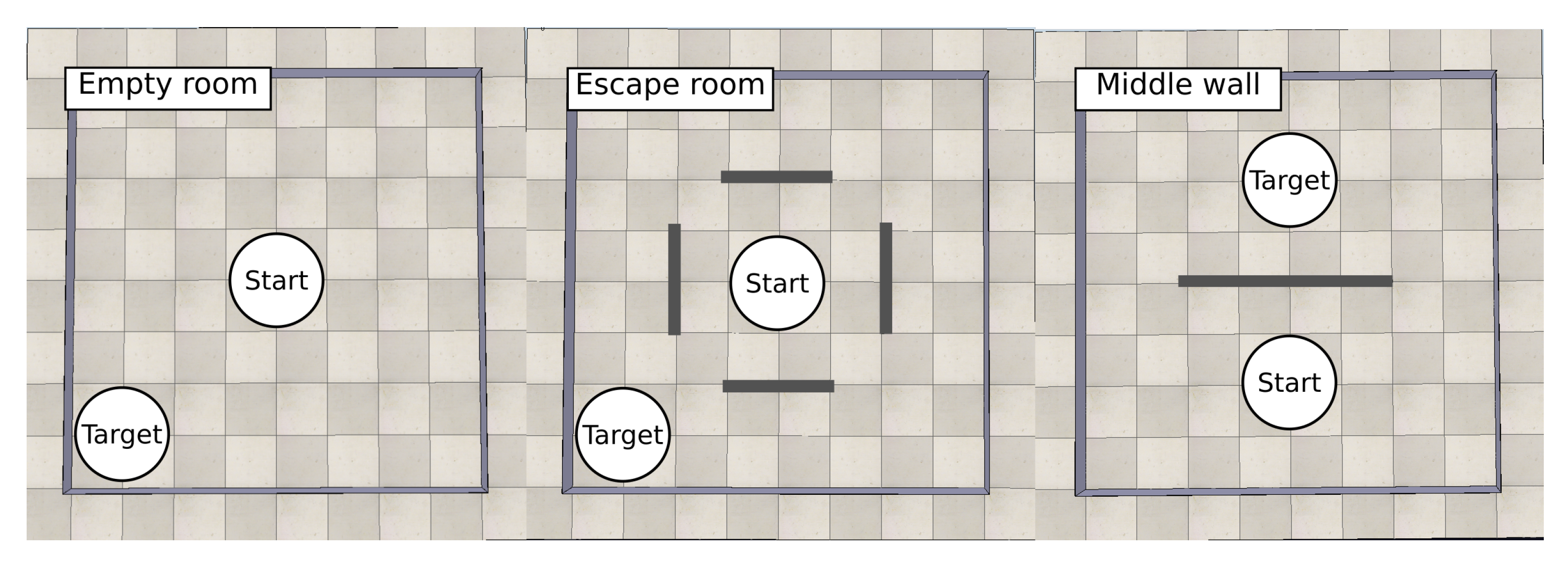
In this navigation task, the robot starts at the origin and has to reach a target. At the target there is a beacon. The robots are evaluated in three different environments (
Figure 6):
empty arena,
escape room and
middle wall. Each of these environments will illuminate the necessary key features in the robots to solve each of the environments. For instance, for the
empty arena, any body plan with actuators has a good probability of solving the task, whereas, in the
escape room, the robots will need to have sensors to avoid the walls and be small enough to move through the gaps in the walls. In each experiment, the robot is controlled by an Elman neural network [
25].
We compare two different methods for finding a controller for a given body plan: random sampling and learning.
Random Sampling
For this experiment, Elman networks with 8 hidden neurons are randomly initialized with LHS for each body plan. This experiment is used as a benchmark and to identify whether any body plans can solve tasks with random controllers. A total of 100 random controllers are generated for each robot in the bootstrap population. Each evaluation has a length of 60 s.
Learning
In these experiments, the Novelty-driven Increasing Population Evolutionary Strategy (NIP-ES) algorithm is used to train a controller for each robot in the bootstrap population, based on our previous work [
26]. The NIP-ES algorithm is a modified version of the increasing-population Covariance Matrix Adaptation Evolutionary Strategy (IPOP-CMAES) [
27]. The IPOP-CMAES algorithm restarts whenever a stopping criterion has been triggered. When the algorithm restarts, the population is doubled. NIP-ES has custom stopping criteria and also includes a novelty score as an additional objective. Complete details of this method, including the stopping criteria and parameter values, can be found in [
26]
Learning finishes for a single robot when: (a) the budget of 1000 evaluations has been reached, or (b) the robot has reached the target, or (c) the robot has not moved in 50 evaluations. The robot has reached the target when the robot is 0.141 m away from the target which is equal to a fitness of 0.95 (the fitness is normalised using the maximum distance possible in the arena, namely the diagonal of the arena: m). The length of each evaluation is 60 s.
As in the previous experiment, the controller is an Elman network with 8 hidden neurons and context units. The number of inputs corresponds to two times the number of sensor organs on the body plan, because each sensor organ outputs two signals (see
Section 3.1.1). The number of outputs is equal to the number of actuators, i.e., number of joints and wheels.
3.3.1. Experiments and Results
The objective of the experiments in this section is to evaluate and identify the necessary attributes in the robots to solve the environments. For this, the clustering-random method is used to select the bootstrap population for the feature descriptor and the LHS descriptor. The latter descriptor is used as a benchmark. A total of 15 repetitions are shown in this section.
Random Sampling of Controllers
In this experiment, 100 random controllers are generated with LHS for each robot in the bootstrap population. These robots are then evaluated in each environment (
Figure 6). The length of each evaluation is 60 s. The results can be found in
Table 6 and are described next.
The feature descriptor provides the highest number of robots closer to the target for any environment, and this is because of the diversity in the population. The empty arena has the highest number of robots reaching the target. This is because it is the easiest task, with no obstacles in the way, therefore the likelihood of reaching the target is high. This is not true for the escape room and middle wall, where robots require more complex controllers and body plans to solve these environments.
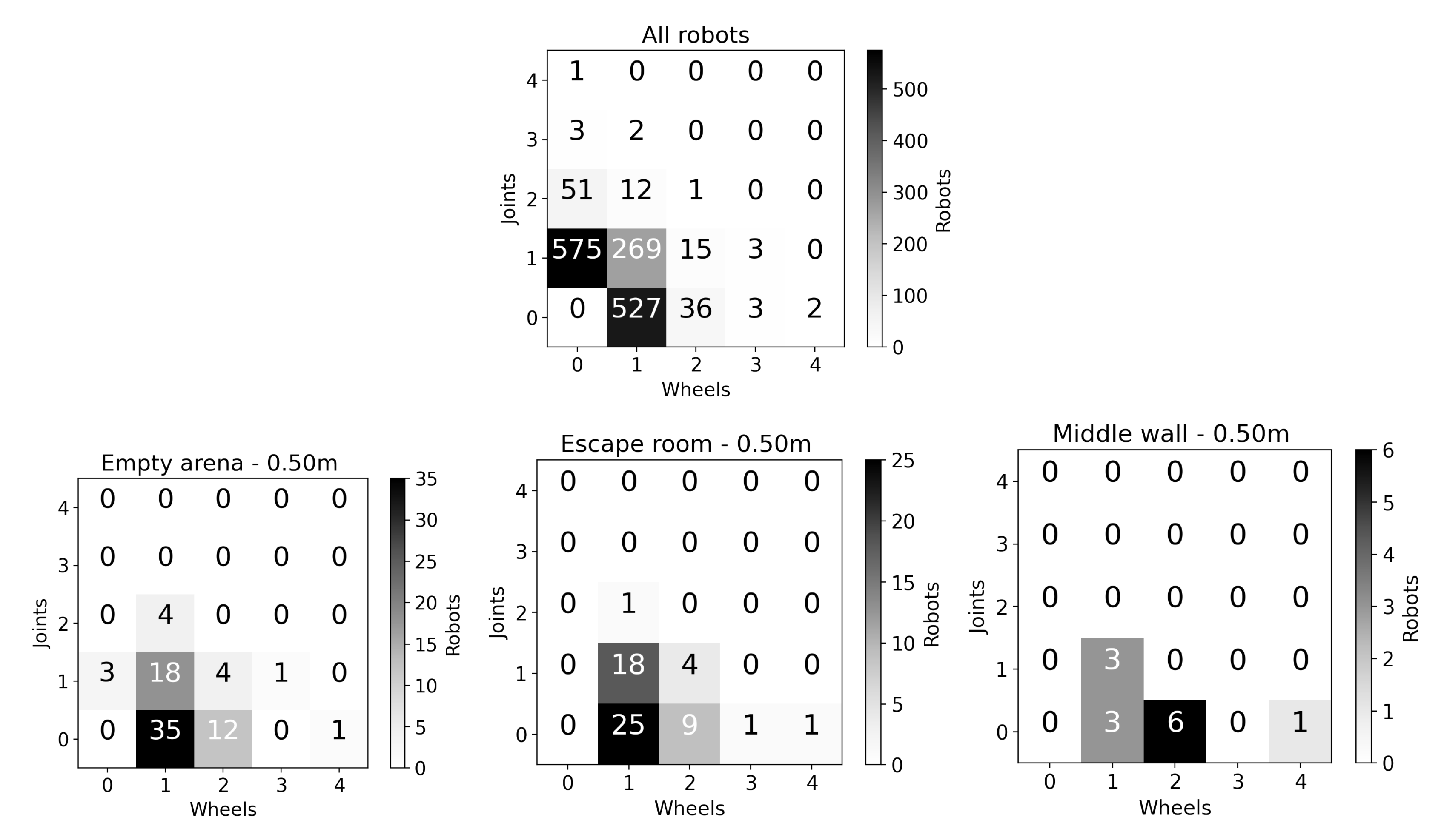
The number of robots with different organ combinations are illustrated in
Figure 7. Most robots in all the bootstrap populations have only one wheel or one joint (top figure). The main attribute required for the robots to get close to the target in the
empty arena is to have wheels. This is because the robots can orbit their way to the target. For the
escape room, some robots need joints to reach the target. Wheeled robots get trapped by walls easily, whereas robots with joints are less affected by this. Robots need two wheels to solve the middle wall environment, as differential drive robots are easier to control to solve this kind of problem.
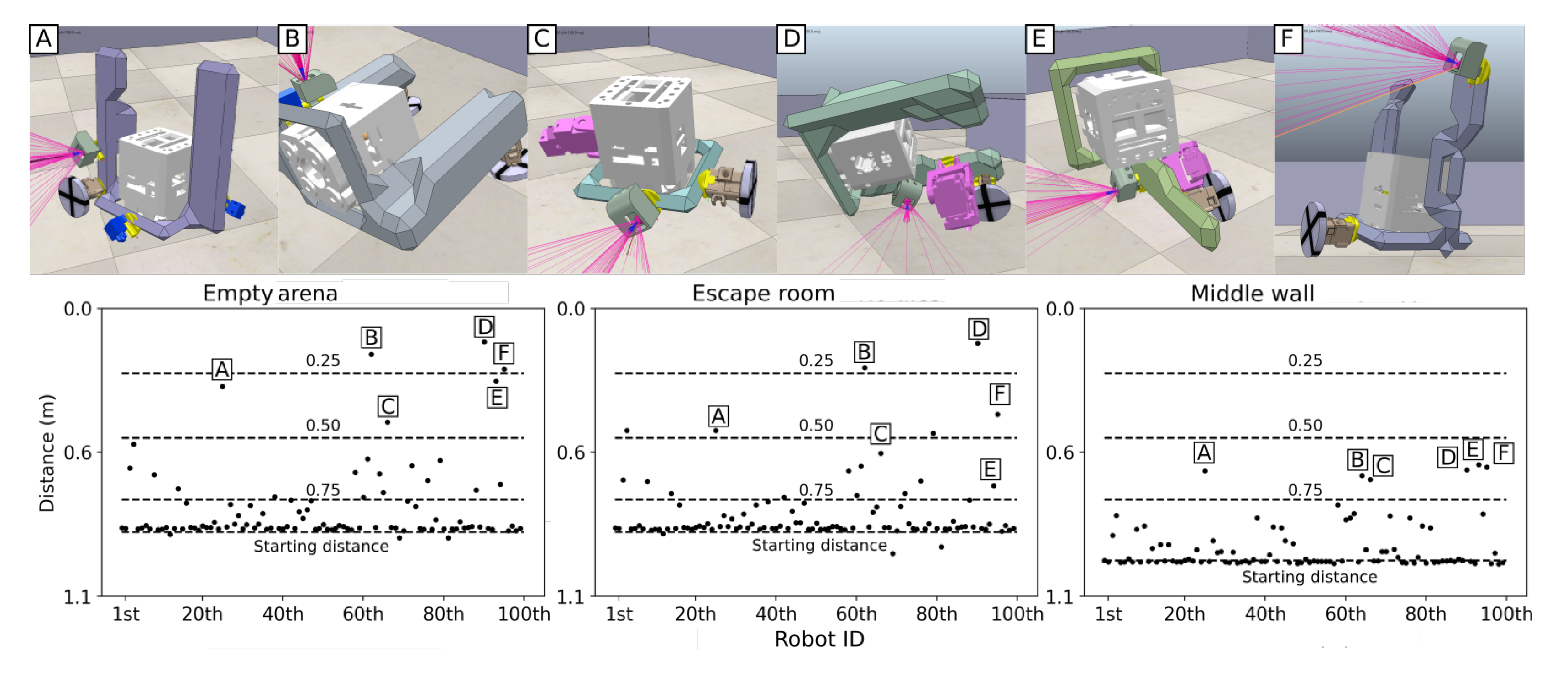
The robots that have a good performance in a simple environment (empty arena) seem to also have a relatively high performance in more complicated environments (escape room and middle wall).
Figure 8 shows the performance of each robot in one bootstrap population. Some robots that did well in the empty arena keep doing well in the escape room and in the middle wall room, just with a reduction in performance. This reduction in performance might be caused by (1) the controller not being good enough to solve the second environment and/or, (2) the physical attributes of the robots not being suitable for the second environment.
In conclusion, the body plans play a key role in solving the navigation task in different environments. Wheeled robots are shown to have a good performance in solving the given environments.
Learning a Controller for a Body Plan
A learning algorithm (NIP-ES) with a budget of 1000 evaluations was applied to each robot in the bootstrap population to gain more insight into the quality of each body plan and identify the ratio of robots able to solve the navigation task. The experiments were conducted first with a bootstrap population obtained through random sampling, and then with a population obtained using novelty search. Robots were selected using the cluster-random method in each case.
As shown in
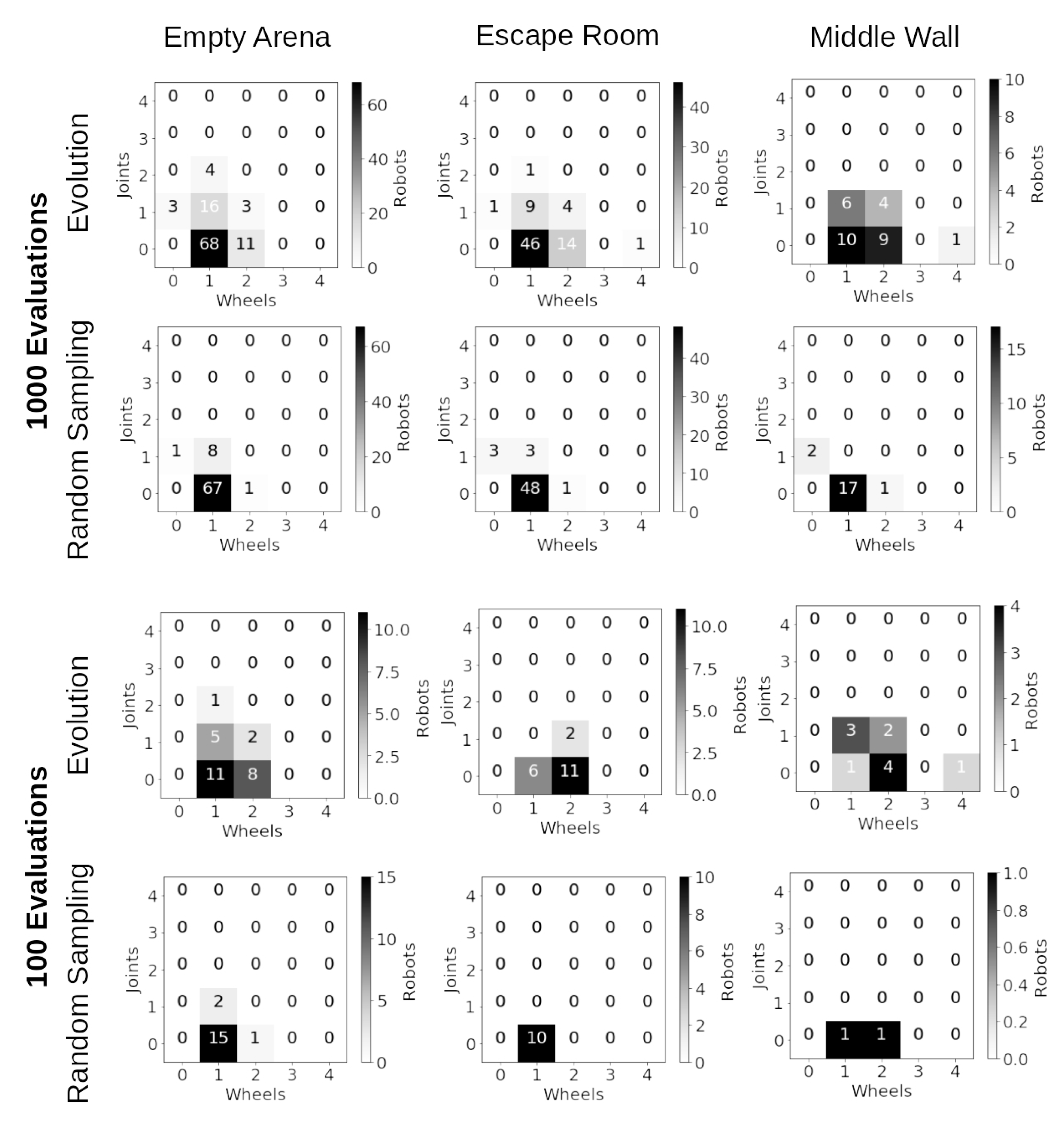
Table 7, in the histograms of
Figure 9, and in
Figure 10, there are more robots able to complete the task in the populations obtained with novelty search compared to those formed by random sampling.
Table 7 shows the median number of robots able to approach the beacon at a distance less than 0.75, 0.5, 0.25 and 0.141 m. 0.141 m corresponds to a fitness of 0.95, which is the minimum value required to complete the task. With either a budget of 100 or of 1000 evaluations, there are in both cases significantly more robots in each distance category than in the case of the randomly sampled robots.
Moreover, the diversity of body plans in terms of number of wheels and joints is greater in the population obtained with evolution as shown in
Figure 9, which shows the number of robots sorted by their numbers of wheels and joints. The first two rows correspond to the population obtained with evolution, and the last two rows the body plans obtained by random sampling. The histograms also show the number of robots capable of completing the task with budgets of 100 and 1000 evaluations.
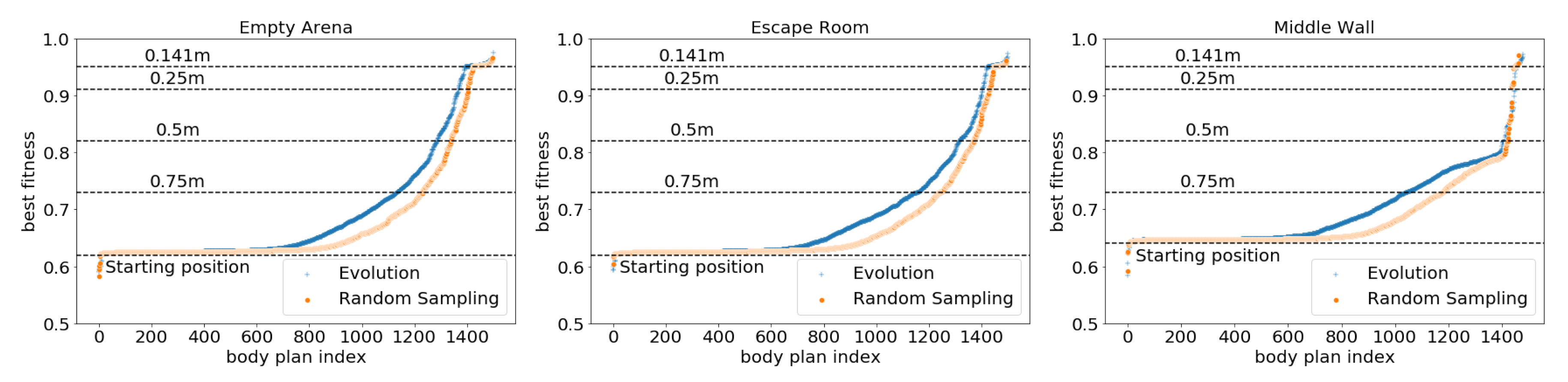
Finally, these results are confirmed by
Figure 10 which shows the best fitness for all the body plans of all replications. There are more robots able to move in the population obtained with evolution than with random sampling: 841, 847 and 903 with evolution versus 708, 705 and 729 with random sampling in the empty arena, escape room and middle wall, respectively.
A side result of the experiments described in this section is to observe the benefit of using learning over just sampling controllers randomly. The NIP-ES algorithm with only 100 evaluations is able to find more robots that complete the task than with the 100 random-sampled controllers shown in the previous section (see
Figure 7 and
Figure 9 and
Table 6 and
Table 7). However, 1000 evaluations is needed to reach the full potential of learning. The number of robots that complete the task with 1000 evaluations is nearly 4 times higher than with 100 evaluations. Moreover, the number of robots and the diversity of their body plans are higher with the population obtained by evolution than the one obtained by random sampling.
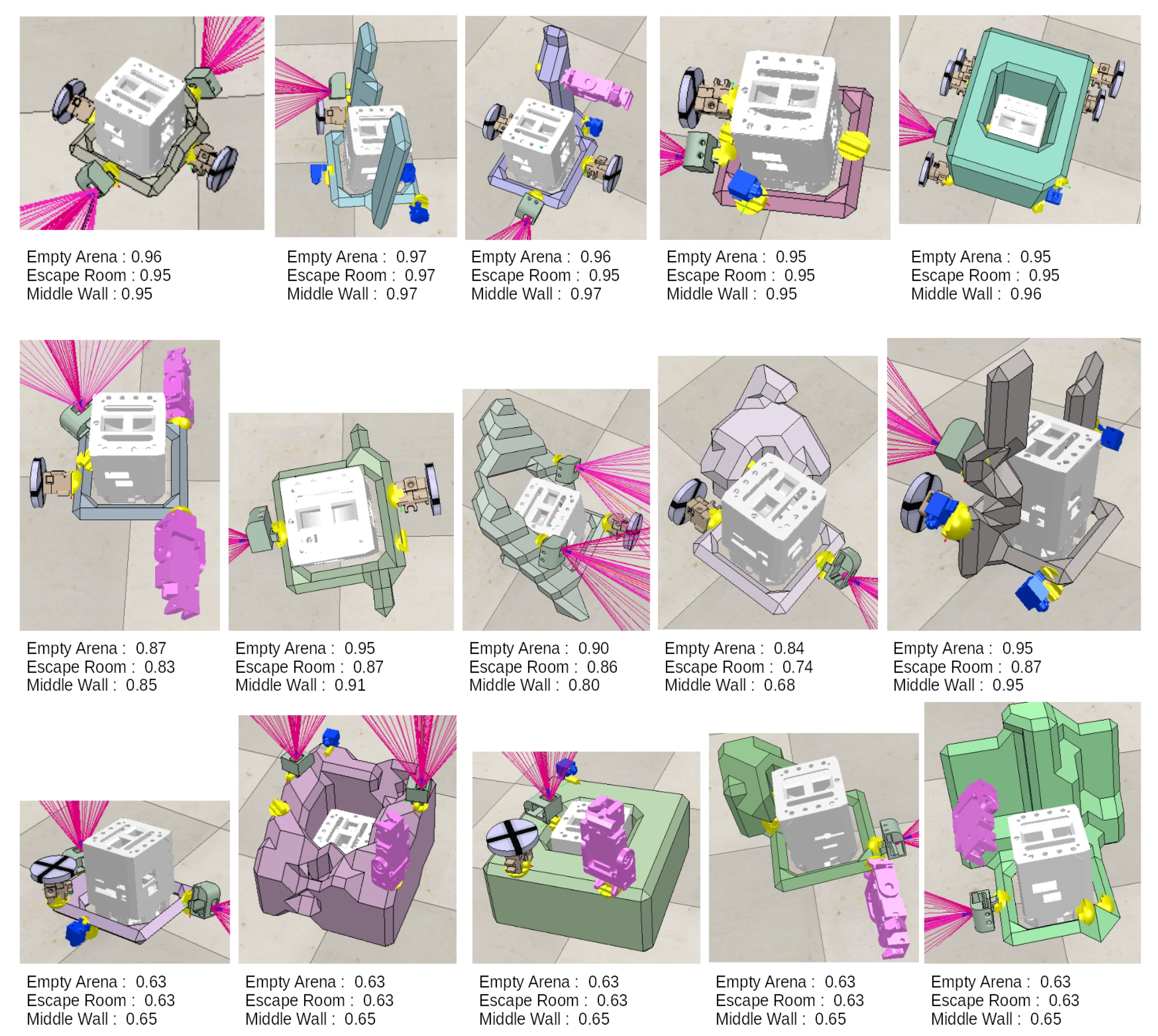
Figure 11 shows fifteen examples of robots’ body plans. The first row corresponds to the successful robots, the second row corresponds to the robots that can move but cannot reach the target and the last row corresponds to the robots that are incapable of moving. Thus, this figure highlights the diverse set of body plans produced by the body plan generation step. As shown in
Figure 9, the number of wheels plays an important role in solving a navigation task. The first row shows the robots with multiple wheels on the ground, and each of these robots have a fitness above 0.95 in all the three environments. The second row shows only robots with one wheel, and the fitness of each robot is more variable in all the three environments. Lastly, the third row shows robots with no actuators that touch the ground.
3.4. Body Plan + Controller Evolution
In order to investigate whether a morph-neuro evolutionary algorithm that simultaneously evolves both body plan and control can be improved by bootstrapping in the manner described above, we conduct further experiments using the following method.
The genome of each robot in the population is divided into two parts: a body plan and a controller. The body plan part follows the same architecture as shown in
Section 3.1.1. The Hyper-NEAT algorithm is used to evolve the controller [
28]. Each body plan is linked with a controller that is indirectly encoded using a CPPN. The decoded controller is a feed-forward neural network with 4 hidden neurons. The decoding takes place as follows.
A feed-forward neural network is produced by connecting the inputs from the sensors with the output of the joints and wheels. The CPPN generates the weights of these connections. For this, the coordinates of the sensors and the actuators are used as input for the CPPN, and the output defines the weight between these connections. A CPPN can thus be used to generate the neural network for any type of body plan, regardless of the number of inputs and/or outputs.
3.4.1. Experiment and Results
In this section, the body plan and the controller for each robot are evolved. The body plan and the controller are each encoded in a separate CPPN. During evolution, operators are applied separately to each CPPN.
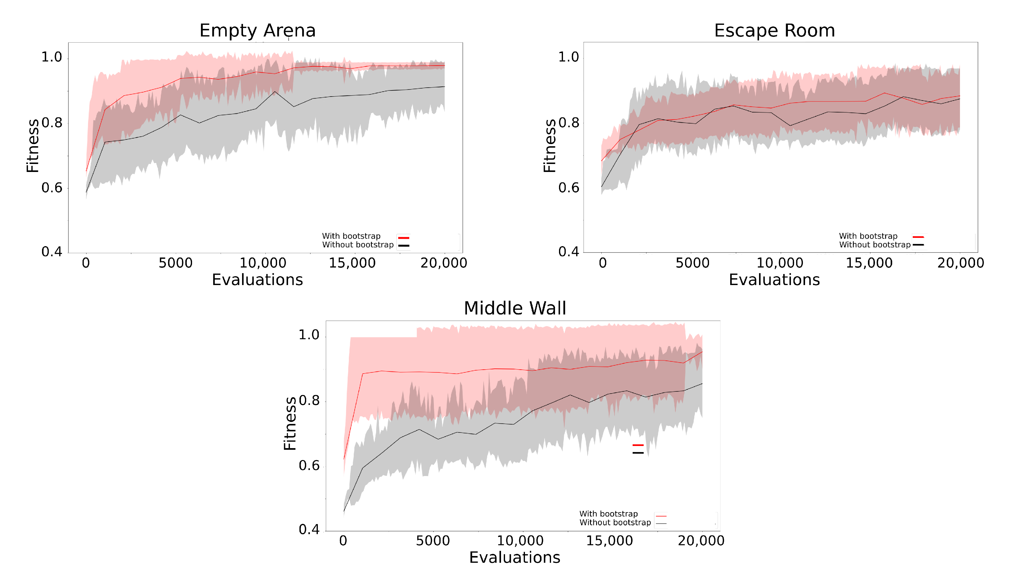
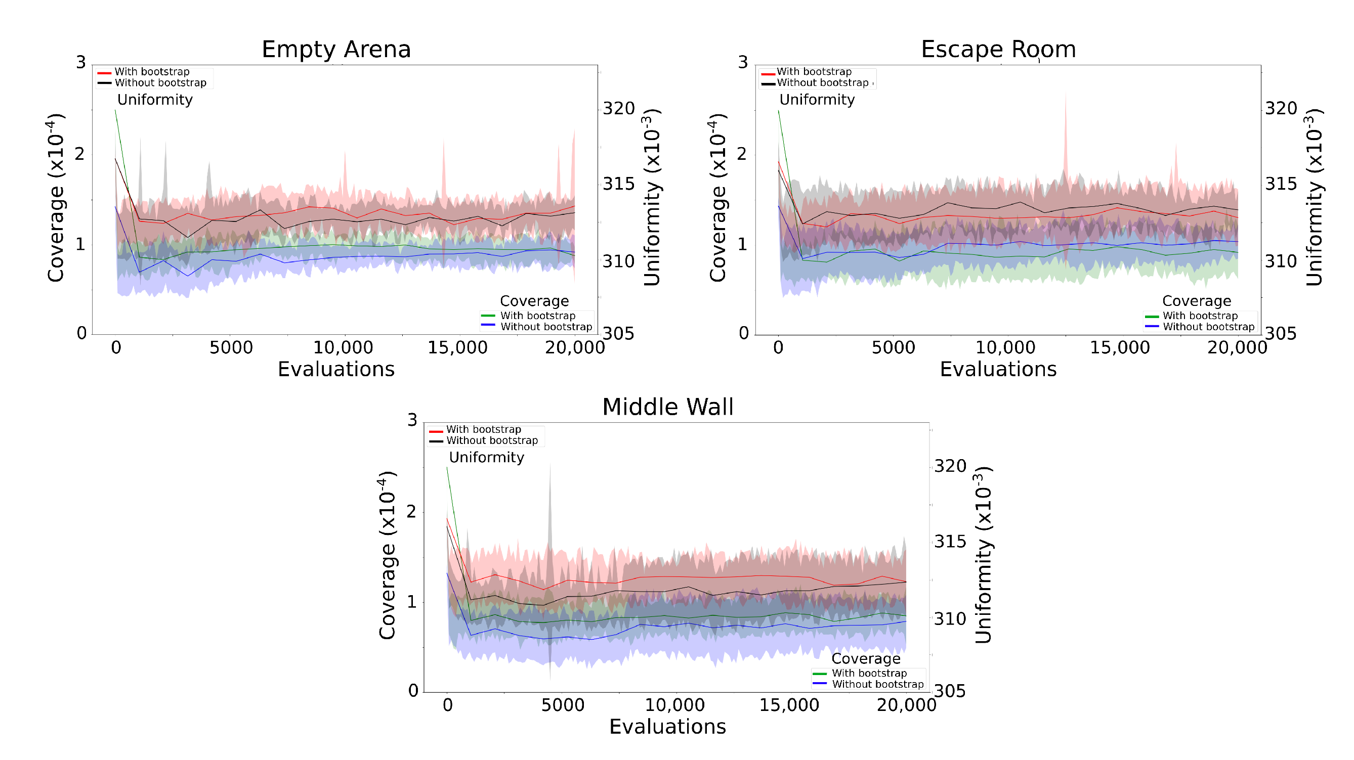
Figure 12 shows fitness, coverage and distribution convergence plots for all the environments (empty arena, escape room and middle wall).
The fitness convergence plots are shown in the left column from
Figure 12, where fitness measures the proximity of a robot to the target. In the empty arena and middle wall environments, the bootstrap method results in a higher fitness and diversity than that of a randomised starting population. However, in the escape room, it appears that there is no difference between these two methods (bootstrap population and randomised population). This might be because it is difficult for the robots to reach the target, given that the robots are relatively big: this means they can become trapped by, or stuck on the walls, making it harder for the evolution to converge to a high-fitness solution. Therefore, in this instance, the bootstrap population method does not show any advantage. This is consistent with the results shown in
Table 6 and
Table 7 and
Figure 11, where the robots in the escape room exhibit a lower performance than the robots in the empty arena and middle wall environments.
Overall, the use of the bootstrap population appears to decrease the number of evaluations required for the evolution to converge to a solution. In addition, the coverage of the body plan search space is higher with the bootstrap than with a randomized population.
3.5. From Virtual to Physical: Fabricating Robots
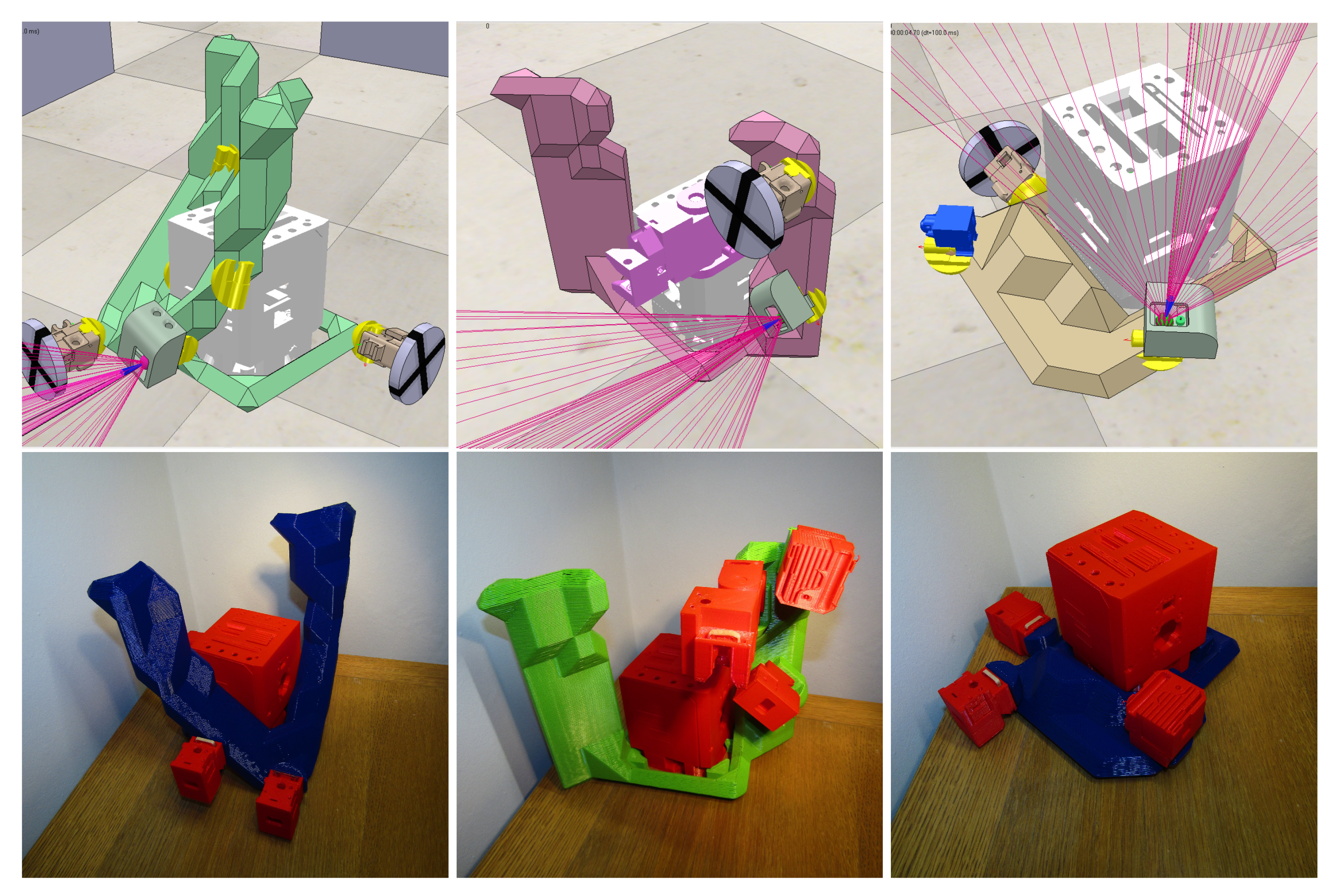
The main goal of this section is to present some examples of fabricated physical robots (The performance of the physical robots has not been evaluated, as the organs are still in development.) from virtual evolved robots. The robots are shown in
Figure 13, demonstrating that virtual evolved robots with different features can be fabricated in the physical world.
The robot in the first column had the best performance of the three robots shown. This is because this robot evolved a two-wheeled differential-drive mechanism, and this kind of robot has been proven to be relatively easily to control. The robot in the second column had a better performance than the previous one. The robot falls over because all the mass is concentrated in the top part. The robot uses the wheel to move in the environment and the joint organ to change direction. The robots in the third column had poor performance in the simulations. This is because the only behaviour this robot can have is to rotate on the spot.
4. Discussion
In this paper, a novel method to generate a bootstrap population of diverse robots that can be autonomously fabricated is introduced. There are three evolutionary processes at play. First, a novelty search algorithm is used to evolve a large list of robots, from which a subset of robots is selected to form a bootstrap population. Secondly, a learning algorithm (NIP-ES, [
26]) is applied to the bootstrap population to learn a controller for these robots, to gain insight into the potential capabilities of the bootstrap population. Finally, the bootstrap population (of body plans) is used to form the initial population of an evolutionary algorithm by pairing each body plan with a random CPPN that generates a controller. Starting from this bootstrap population, an evolutionary algorithm is run to find a robot capable of solving a maze navigation task, simultaneously evolving both body plans and controllers. The key results from this paper are described next.
The choice of body plan descriptor influences the complexity and diversity of the body plans evolved (Section 3.1.3). Used in conjunction with novelty search, the descriptor defines the physical attributes of a robot, including skeleton complexity and the number and type of organs. In this paper, the robots were evolved for novelty with three different descriptors:
feature,
symmetry and
spatial. The most complex skeletons were evolved with the
spatial descriptor as more of the elements of the descriptor are associated with the skeleton properties. The
feature descriptor provided the highest number of robots with different numbers of organs and this is because the organs have a heavier weight in this descriptor. The
symmetry descriptor sits somewhere between these. The body plan descriptor plays a key role defining the final physical properties in the robots. Therefore, the body plan needs to be carefully designed to suit the task for the robots.
The method used to select the bootstrap population influences the final diversity and numbers of organs in the population (Section 3.2.1)—Four different algorithms to select the bootstrap population were compared (
LHS,
clustering-random,
clustering-sorting and
sparseness-sorting) with the k-means clustering algorithms providing the best bootstrap populations with the highest number of diverse robots.
LHS was the method with worst performance. The clustering algorithms were able to successfully classify the robots in clusters with different properties according to the traits in the
feature descriptor.
Body plans evolved with the feature descriptor exhibit better navigation behaviours with both randomly assigned controllers and learned controllers than body plans that are randomly generated (Section 3.3.1). The behaviours of the robots in the final bootstrap populations were evaluated in three different environments, with randomly generated controllers and with a learner, and this was compared with randomly generated robots. The evolved body plans had a higher number of robots getting closer to the target than the randomly generated body plans. This means that the bootstrap population are diverse enough to have enough body plans to solve the environments for this paper without the need to evolve the body plan any further. For more complex environments, further evolution of the body plan might be required.
Bootstrapping an EA with an initial population selected for diversity reduces the number of evaluations necessary to converge to the solution, when a population of robots with controllers and body plans is evolved (Section 3.4.1). It takes a larger number of evaluations for an evolutionary loop to converge to a good solution with a random initial population than with a population evolved for novelty. This is because when robots are evolved for novelty, there is high likelihood that one of the robots in the population will have a good performance in the environment, as the population is more diverse. The reduction in number of evaluations will become very important when robots are evolved for more complex environments.
Overall, the body plan generation creates a better initialisation population than a population generated at random. The evolved populations are diverse enough to have some body plans in the population that are capable of solving some environments without the need of further optimisation. In addition, an evolutionary loop starting with a bootstrap population converges quicker to the solution than with an initial population generated at random. Finally, all of the robots in the experiments can be autonomously fabricated by the Robot Fabricator.
5. Concluding Remarks
Employing artificial evolution for discovering well-performing and novel robots for complex environments and tasks has great potential [
29,
30,
31,
32]. However, forced by technical limitations, existing work in evolutionary robotics is mainly limited to simulations and the physically constructed robots—if any—are very simple. Thus, the transition from the virtual domain to the real world is yet to be made.
The Autonomous Robot Evolution project represents a milestone on the long road ahead. The overall goal of the project is to make the transition to the real world and develop a system where physical robots evolve. A key objective to this end is to automate the fabrication of complex robots with partly 3D-printed bodies, a CPU and several sensors and actuators. The hands-free fabrication of robots is difficult, but the technology is becoming available [
2,
8,
9].
In this paper, we identify a new problem that does not occur in simulated evolutionary processes. This problem, dubbed the fabrication challenge, is rooted in the fact that autonomous robot reproduction inevitably implies constraints regarding the evolved robots. In short, the robots need to be not only be conceivable but also autonomously fabricated. This implies an essential condition for the robotic evolution process: the initial population needs to consist of manufacturable and diverse robots. The chief contribution of this paper is a novel method to generate this initial population. To be specific, we describe and investigate a method that considers not only morphological constraints but also behavioural requirements of the generated body plans and the diversity within the set of generated body plans. To assess the merits of this method, we ran a full robot evolutionary process where the morphologies (body plans) and the controllers (brains) of the robots were evolved together. The experiments showed that initialising the first generation by our method improves the efficiency and the efficacy of evolution.
In this method, a large pool of diverse manufacturable robots is generated. Then, a subset of diverse and viable robots is selected from this list to seed the evolutionary process. The results shown in this paper can be summarised as follows: (a) the descriptor used defines the physical attributes of the final list of robots evolved; (b) the method used to select the subset of robots (population) define the diversity of the same population; (c) the initialization of the population is better with a pre-evolved list of robots than a random population and (d) the speed of convergence increases when the initial population is selected from evolved robots.
Further work will explore the enhancement of the genome decoder, with the goal of increasing the number of organs generated in the evolved robots. In addition, new methods of evolution of body plans and controllers will be explored. Most importantly, the physical robots will be evaluated in a real-world setup and any resulting reality gap measured, with the objective of then developing new methods to decrease it.

 ,
, 


