On the Benefits of Color Information for Feature Matching in Outdoor Environments

Computer Engineering Group, Faculty of Technology, Bielefeld University, D-33615 Bielefeld, Germany
Robotics 2020, 9(4), 85; https://0-doi-org.brum.beds.ac.uk/10.3390/robotics9040085
Submission received: 30 July 2020
/
Revised: 3 October 2020
/
Accepted: 5 October 2020
/
Published: 11 October 2020
(This article belongs to the Section Intelligent Robots and Mechatronics)
Abstract
:The detection and description of features is one basic technique for many visual robot navigation systems in both indoor and outdoor environments. Matched features from two or more images are used to solve navigation problems, e.g., by establishing spatial relationships between different poses in which the robot captured the images. Feature detection and description is particularly challenging in outdoor environments, and widely used grayscale methods lead to high numbers of outliers. In this paper, we analyze the use of color information for keypoint detection and description. We consider grayscale and color-based detectors and descriptors, as well as combinations of them, and evaluate their matching performance. We demonstrate that the use of color information for feature detection and description markedly increases the matching performance.
1. Introduction
Autonomous lawn-mowing under visual guidance is a complex task for outdoor robots. One of the basic elements is a visual navigation system that enables a systematic covering of the entire working area. In outdoor environments, varying illumination conditions as well as seasonal changes and nonplanar terrain pose multiple challenges to a visual navigation system. For the class of methods that we are interested in, the computation of the spatial relationship between arbitrary views (“home vectors”) is required. Therefore, we focus on feature matching without restricting the search space by feature tracking and study the effect of incorporation of color information in order to improve feature matching. Furthermore, we concentrate our study on the performance in the context of domestic gardens and lawns near public buildings.
Feature detection, description, and matching are fundamental parts of feature-based visual navigation. A wide variety of feature detectors and descriptors have been proposed in the last decades, for both grayscale and color images. A review and evaluation of different detectors and descriptors is beyond the scope of this article; we refer to [1] for grayscale images and [2] for color images. Most evaluations of different feature detectors and descriptors are found in the context of object recognition, image registration, camera calibration, and three-dimensional world reconstruction. Studies regarding the impact of different feature detectors and descriptors on the accuracy of visual simultaneous localization and mapping (vSLAM) are mainly restricted to indoor environments, grayscale features, negligible camera in-plane rotations, and short baselines between images [3,4,5,6].
In outdoor environments, autonomously navigating robots have to solve additional problems as compared to indoor environments. Incorporating color information is an obvious option to improve feature-based methods, as the main purpose of color descriptors is to increase the photometric invariance and the discriminative power. Previous studies on color descriptors have been limited to computer vision tasks, such as object and scene recognition, and they do not cover typical scenes for lawn-mowing robots (e.g., [2,7]). In this article, we focus on the impact of incorporating color information in feature detection and description measured by an evaluation criterion suitable for a subsequent random sample consensus (RANSAC) [8] step. Therefore, we select a widely-used feature detection and description method (SIFT [9]), which we still consider as state-of-the-art, and analyze the incorporation of color information. Instead of comparing different color feature detectors and descriptors, we retain the main components of the method and focus on the use of additional color information. We evaluate the methods on outdoor image datasets regarding their inlier frequency as evaluation criterion. In the feature matching step, no tracking is performed, as this is not possible in the intended application scenario. In the context of feature-based methods, a vast amount of published literature exists, and the use of color information in robotics vision is no new approach (e.g., [10,11]), but our study focuses on a specific use case with special characteristics: feature matching in fisheye images for pose estimation in outdoor environments.
In [12], Dzulfahmi and Ohta present a performance analysis on image matching in outdoor environments. The main focus of this study is the tolerance of the feature detector and descriptors against illumination changes by matching of images to images of the same scene at different illumination conditions. This evaluation is performed in a teaching and playback setup, but it also includes only grayscale methods. In a similar teach-and-repeat context, Krajník et al. [13] also analyze feature detection, description, and matching in outdoor environments. Likewise, the evaluation is based on grayscale features, but the focus lies on long-term matching, despite strongly changing appearances in outdoor scenarios due to weather conditions and even seasonal changes. In this underlying context, the robustness to the change in appearance is more important than viewpoint changes or non-planar surfaces. In [14], Valgren and Lilienthal address appearance-based topological localization for seasonal changes. It is stated that feature matching that is based on SIFT or SURF alone is not sufficient for visual localization across seasons. The authors propose the additional use of epipolar constraints in order to solve single-image localization under these conditions. Other feature-based approaches for visual navigation in outdoor environments typically involve tracking the detected features across time, such that the search space of the matched features is restricted (e.g., [15]).
Contrary to the above-mentioned studies, we focus on the following three main aspects: (1) benefits of color information for feature matching, (2) environments that are typical for a robot navigating in lawn-mowing scenarios, which include long baselines (ranging from approximately one to 30 meters) and camera rotations, and (3) images that are captured on different locations that are matched to compute relative pose estimates without feature tracking. Many of the state-of-the-art visual navigation approaches that are based on feature matching use feature tracking to restrict the search areas for each feature and thereby prevent strong outliers. In our application, feature tracking is not suitable, as we compute home vectors between arbitrary views from a topological map and not only along the driven path.
These aspects arise out of the intended use case in an autonomous lawn-mowing task that we sketch out here. The main task of the robot is to systematically cover a predefined lawn area aiming for complete coverage with minimal overlap. This approach is built on previous work on visual navigation for an autonomous cleaning robot [16]. The main difference is the transition from indoor to outdoor scenarios, which implies several challenges; however, the basic approach is equal. The robot uses an upward facing camera with a fisheye lens to build a topo-metric map of its environment, which allows for a systematic covering of the entire area. The map is built anew for each lawn-mowing run and, thus, only needs to handle changes within the time period of one run. This includes changes in weather, illumination, and small changes in the environment, but no longterm changes, such as seasonal variations. One fundamental module for this map building is the computation of home vectors to previously visited views, which is addressed in this article. Furthermore, we use fisheye images to detect and describe image features, without a preceding mapping to azimuth-elevation format. Alongside advantages, e.g., a larger field of view and the separability of rotation and translation, fisheye images also pose challenges, like smaller and more distant objects or problems with lighting conditions.
We ground our approach on a camera as main sensor, which comes at low costs and can be used for additional tasks of the complete system, like obstacle avoidance or terrain classification. Besides visual navigation with cameras, global navigation satellite system (GNSS) receivers are alternative sensors for autonomous systems in outdoor environments. However, GNSS measurements strongly deteriorate in urban canyons due to signal blockage and reflections, which can result in positioning errors up to 100 m in dense urban areas [17]. Thus, GNSS based navigation requires sophisticated approaches in urban areas and they often use additional sensors to correct the measurements (e.g., [17,18]).
Recently, the advances in the context of deep learning led to approaches that produce learned feature descriptors in contrast to the classical, handcrafted descriptors. We refer to [19] for a comprehensive and systematic review on the development from handcrafted to learned features in image matching. However, approaches that are based on deep learning require large datasets with annotated ground truth values as well as powerful GPUs onboard the autonomous system [20]. Promising results in the context of deep learning based pose regression are, for example, reported by Kendall and Cipolla in [21]. The current lack of suitable, annotated training data (in our case fisheye images with ground truth positions) and the still existing deficit in accuracy (see [21]) justify this study on the use of color information in combination with classical feature detectors.
2. Feature Detection and Description
In outdoor environments, changing illumination conditions as well as cluttered and repetitive scene parts pose challenges to state-of-the-art feature detectors and descriptors [12,22,23]. In the context of this paper, we mainly consider environments that resemble typical domestic gardens. These are especially interesting data sets for research regarding autonomous lawn mowing. In such scenarios, large parts of the images contain grass, bushes, trees, or other plants. On the level of features, e.g., leaves that belong to the same or to different trees are difficult to match correctly. Leaves are non-distinctive regarding grayscale values and typically green; nevertheless, additional information in the form of small changes in hue and saturation could be useful. Hence, we analyze whether color information improves the distinctiveness of such kinds of features.
Color information can be incorporated in the feature detection step as well as in the feature description step. Therefore, we analyze different combinations of color and grayscale methods. SIFT [9], which works on grayscale images both for detection and description, is one of the most commonly used feature detectors and descriptors. A variety of color descriptors have been proposed; van de Sande et al. [2] published an evaluation and overview regarding object and scene recognition. Such color descriptors are most frequently computed on keypoints that are detected in grayscale images (e.g., OpponentSIFT [2]). The counterpart to color descriptors are color detectors that use color information to detect interest points in the image and then describe the keypoint regions by using only grayscale information. Stöttinger et al. [24] proposed a keypoint detector, which considers scale invariance based on color information and a close reimplementation adapted to our images is used in this study. Barata et al. [25] analyzed the use of color both in the detection and description step, but only in the context of dermoscopic images for computer-aided diagnostics. Here, we analyze one method from each of the four categories:
2.1. Scale-Invariant Feature Transform (SIFT)
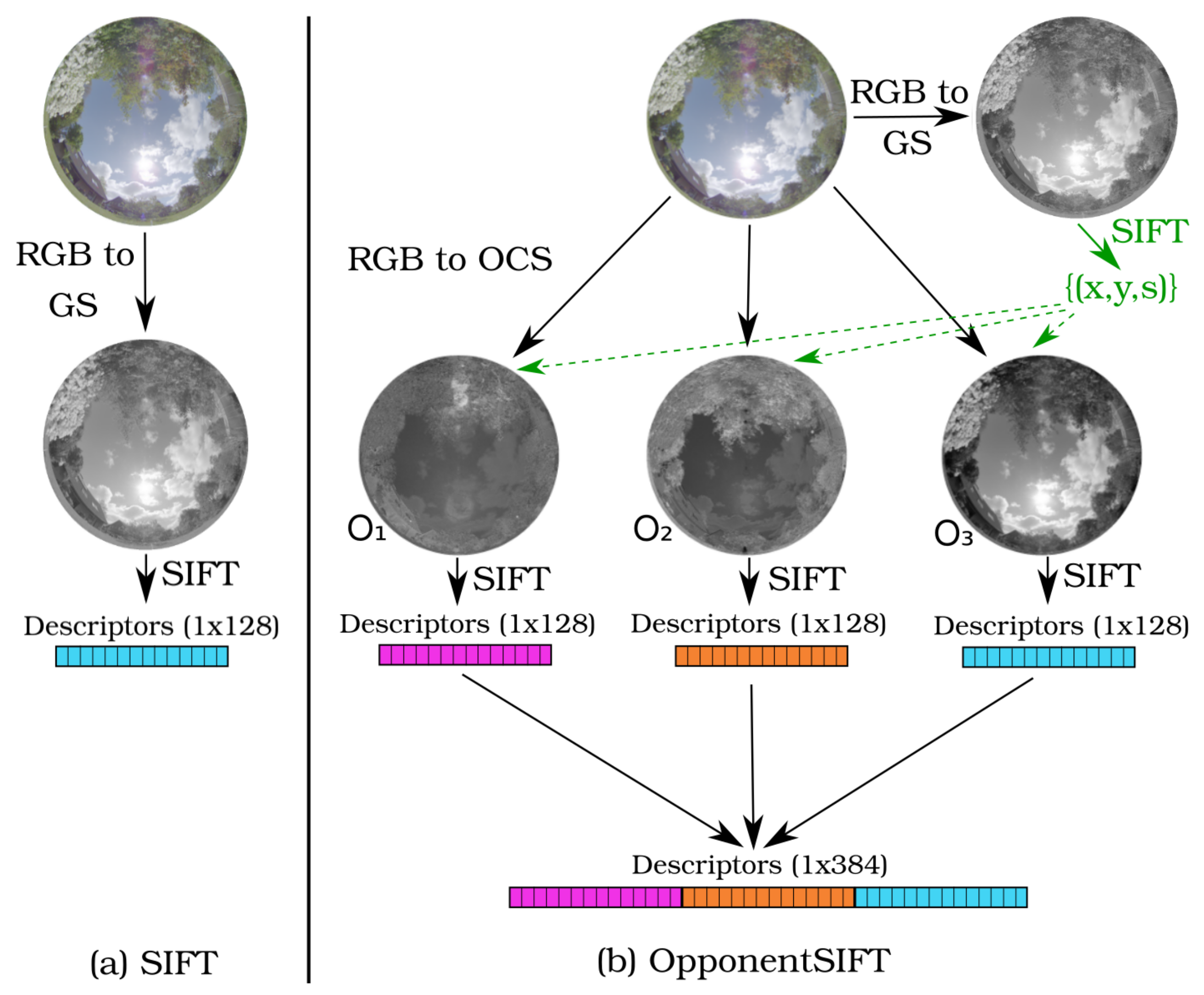
As baseline for our evaluation, we use the widespread scale-invariant feature transform (SIFT) algorithm [9]. We make use of the implementation provided in the OpenCV library in version 3.4.0 [26]. Most of the parameters are left at the default values (i.e. three layers in each octave, the contrast threshold to filter out weak features is 0.04, and the edge threshold to filter out edge-like features is 10.0). The value of for the Gaussian filter of the first octave is reduced to , which corresponds to for color interest points (see Section 2.3) and it is varied in our experiments. The procedure is shown in Figure 1 on the left side for an exemplary image. First, the color input image is converted into a grayscale image by applying the standard conversion . Subsequently, the standard SIFT algorithm is executed on this single-channel image giving a list of feature descriptors each of the size 1 × 128.
2.2. OpponentSIFT
OpponentSIFT [2] extends the description of SIFT features with color information. van de Sande et al., showed that SIFT descriptors are not invariant to light color changes and propose several color versions for SIFT that have different invariance properties. The performance of the descriptors is domain-specific, but OpponentSIFT is recommended if no prior knowledge of the data set is available. OpponentSIFT descriptors are invariant to light intensity changes and shifts.
The input color image is converted into a grayscale image as for SIFT, as shown on the right-hand side of Figure 1. For the detection of features, the SIFT algorithm is applied to this grayscale image. Aside from that, the input color image is converted to the opponent color space (OCS), defined in [27] as
Subsequently, the detected SIFT features are described in all three channels of the opponent color space, thus including color information for channels and , as well as intensity information in channel . The three descriptors of size each are concatenated into a single color descriptor of size . We implemented OpponentSIFT within the OpenCV-framework (built on the available SIFT implementation) with the same parameter values as given above for SIFT.
2.3. Sparse Color Interest Points (CIP)
In this section, we recall the selected approach to incorporate color information in the feature detection process, which is called “Sparse color interest points” (CIP), as proposed by Stöttinger et al. [24]. The main idea of CIP is to extend a multichannel Harris corner detector [28] by adding a scale selection method in order to obtain scale-invariant color features. We reimplemented this procedure to consider the projection of a hemisphere to a circular region on the sensor by the used fisheye lens. The part of the image frame outside of the circular projection area is discarded for all computations. We use the so-called light-invariant points as color interest points [24]. The basis of this method is the shadow-shading-specular quasi-invariant (SSSQI) derived in [27] to enable invariance regarding illumination effects, like shadows and highlights. Basically, this photometric invariance is achieved by appropriate projections in the color space, which decorrelate specular, material, and shadow-shading directions of the color derivatives. On the two channels of the SSSQI, a multi-channel, multi-scale Harris detector is computed.
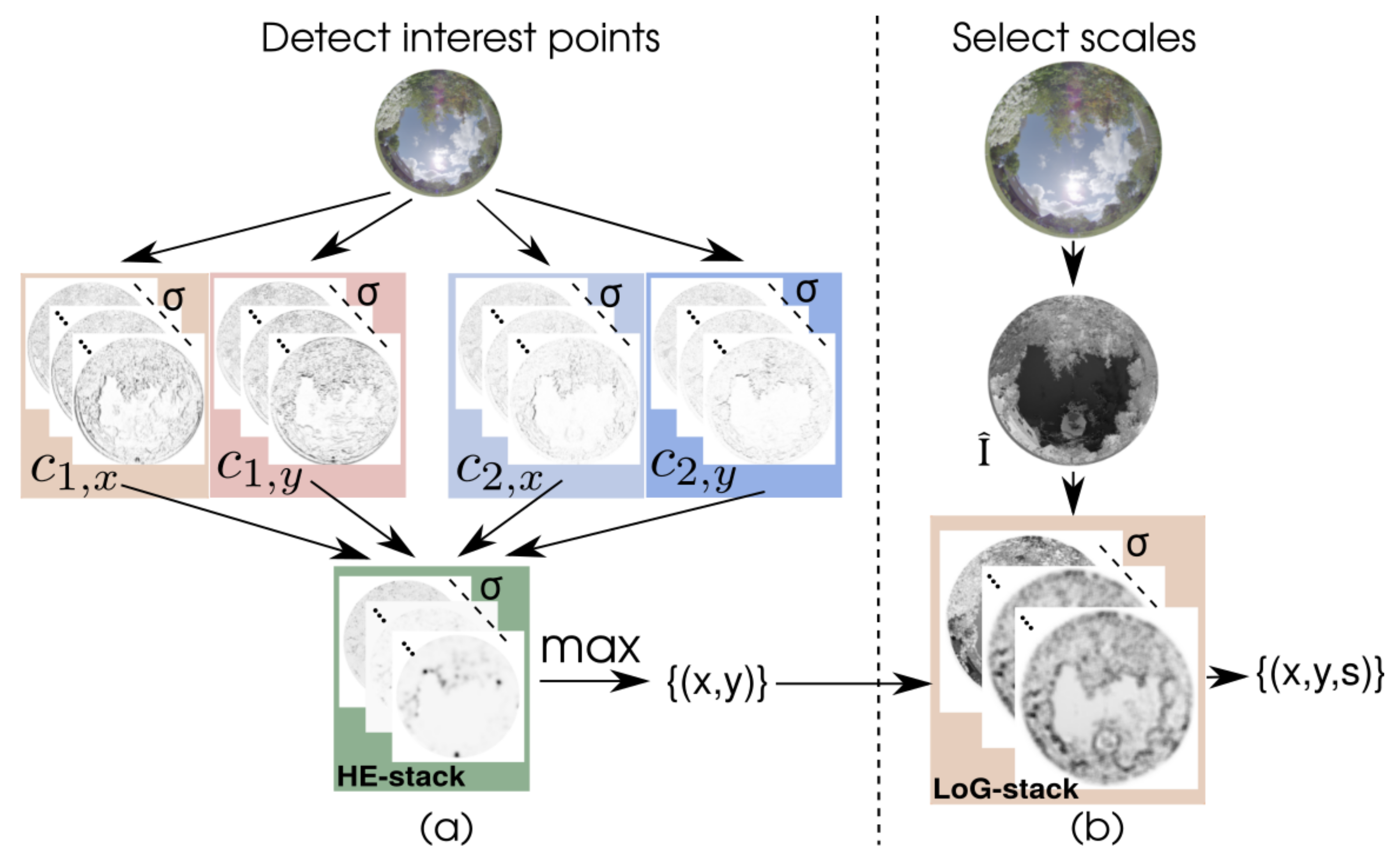
We briefly outline the approach here that is based on the illustration presented in Figure 2. Details of our implementation and the equations are given in the Appendix A. The method combines two processing branches: (a) interest point detection and (b) scale selection. In the first phase, the use of color information in a Harris detector enables the detection of discriminative and repeatable key points in natural outdoor scenes. The incorporation of saliency in the scale selection step of the second phase provides features that are robust to scale-changes [24].
A multi-channel Harris corner detector is computed on the color image for different scale levels for the detection of interest points. Spatial derivatives in x- and y-directions of the RGB-channels of the input image () are calculated and then transformed to the HSI-space to compute the SSSQI. Based on the two channels and of the SSSQI, a color-based second-moment matrix (also known as structure tensor) is computed for different scale factors. A second-moment matrix describes the distributions of the gradients in a given region and it is used here to compute the Harris energy (HE) as corner measure for the interest point detection. The matrices of HE for different scale levels are combined to form a scale space. The intensity channel is discarded for the computation of this HE scale stack. This approach is illustrated in Figure 2a for an exemplary image. The derivatives are visualized as absolute values and normalized to ; small values are white, large values are black. The scale stacks of , , , and comprise the color derivatives in x- and y-direction of the SSSQI on multiple scale levels. Derivatives in the x-direction (, ) result in high values for vertical edges in the image, whereas derivatives in the y-direction (, ) result in high values for the horizontal edges. For the example image, this effect is difficult to distinguish visually, because most of the edges are not exactly aligned with the x- or y-direction, but it is best noticeable at the skyline regions. In the HE-stack, local maxima are searched within a neighborhood of 26 elements, which include eight immediate neighbors within the scale level and nine neighbors from each of the two adjacent scale levels. From all found local maxima, the maxima with the largest HE-value are selected up to a given number of required interest points.
In order to select a characteristic scale for the interest points, a single-channel saliency image is computed and used for a Laplacian-of-Gaussian (LoG) on different scales, as in [24]. Stöttinger et al. [24] motivated the use of the saliency image for scale selection instead of the HE-stack by the incorporation of a global saliency measure in the process. Figure 2b visualizes the scale selection procedure. The saliency image is built on the representation of the input image in HSI color space and it is related to the concept of eigenimages [29]. For potential interest points found in the HE-stack, the characteristic scale level is selected as the scale level , which maximizes the LoG with respect to scale. The radius r of the corresponding size for a subsequent descriptor is computed, depending on and the initial for the Gaussian smoothing kernel of the first scale level.
The main parameters for CIP are the initial standard deviation of the Gaussian kernel for the Harris scale stack , the number of scale levels l, the relation between differentiation scale , and integration scale . We set these parameters to , , and . Additional parameters for the implementation and related equations are given in the Appendix A.
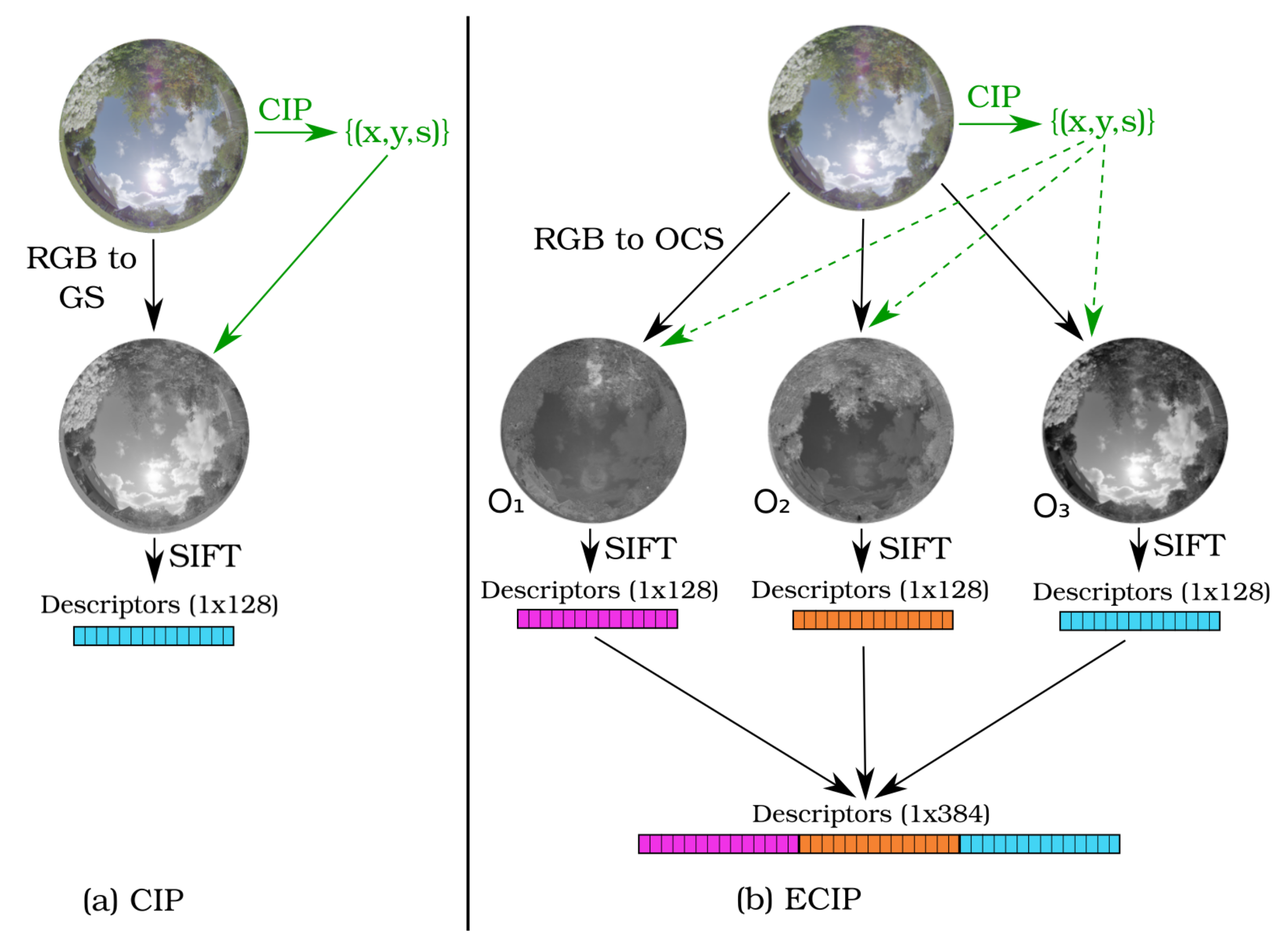
Based on the positions of the interest points and their corresponding sizes, a standard SIFT descriptor [9] is computed on the grayscale image, as illustrated in Figure 3a. For the computation of the SIFT descriptor, we use the implementation that is available in the OpenCV library with the same parameters as above for SIFT (see Section 2.1). For CIP, the color information is used to detect interest points, but it is discarded for the computation of the descriptors.
2.4. Extended Color Interest Points (ECIP)
As an extension, we use CIP, as described above, to find salient keypoints, but additionally use color information for the description step. For this purpose, we combine CIP (Section 2.3) for the detection with OpponentSIFT (Section 2.2) for the description. To the best of our knowledge, this combination has not been analyzed and published before, but it seems to be a natural extension. In Figure 3b, the resulting combined method is shown: the input color image is used to compute the positions and scales of keypoints while using CIP and, for these keypoints, OpponentSIFT is applied to compute color descriptors. We call this approach “Extended color interest points” (ECIP), as color information is relevant for both steps: detection and description.
2.5. Feature Matching
To match the features between two images, we use a simple knn-matcher using the L2-norm and select the best-matching feature candidate. Additionally, we compute the distance ratio that is based on [9] between the best and second-best match, but without rejecting matches with low distance ratios. We use the distance ratio values to sort the matches with regard to their reliability.
3. Evaluation
We performed different experiments to study the effect of color information on feature detection, description, and matching. To evaluate the results, we motivate and describe the applied evaluation methods here, followed by a description of the underlying datasets and the experimental setup.
3.1. Evaluation Criteria
Many different evaluation criteria have been proposed in the context of feature matching. Widely used are the receiver operating characteristic (ROC) curves and precision-recall plots. A first investigation of our data showed strongly imbalanced data sets, i.e., the number of negative matches (true negatives + false positives) is much larger than the number of positive matches (true positives + false negatives). This is caused by the type of the analyzed data sets that comprise images in outdoor scenes at different positions and under varying illumination conditions. There exist many features in one image that are not visible in the other image due to occlusions and the restricted field of view. According to [30], the ROC curves can be deceptive on imbalanced data sets and, thus, are not used here. The recommended precision–recall plots are also used in feature matching (e.g., [1,31]), where recall is computed as
In this equation, the number of keypoints possible to detect is difficult to compute, as it requires knowledge of the visibility of features in the matched images. However, by applying ground truth information, we are only able to recognize features that are no longer in the field of view, but we cannot detect obscured features due to occlusions. This fact would distort the recall value, as the number of obscured features varies throughout the data sets. Similar problems exist for other frequently used evaluation criteria, like repeatability ([32,33]), when applied to our data sets.
Therefore, we focus on a criterion relevant for a subsequent RANSAC step [8] for visual navigation, i.e., our use case. In a RANSAC method, the relevant parameter is the inlier ratio w, which is defined as the fraction of the number of inliers (i.e. data points fitting to the data model) in the data set divided by the total number of points in the data set. The inlier ratio directly influences the number of RANSAC iterations k needed in order to ensure with probability z that at least one outlier-free set is selected. For a model that is based on n points, the number of iterations is computed, as in [8]:
Advanced methods that are based on RANSAC use guided sampling schemes to improve the accuracy and speed (e.g., PROSAC [34]). In the context of a guided sampling, not only the inlier ratio, but also the distribution of inliers within the data set are relevant. In many applications, a priori knowledge about the distribution of inliers is available, but discarded for a subsequent RANSAC step. Concerning feature matching, the matching process provides information on the reliability of each match by analyzing the distance measure between keypoints. This enables the sorting of the samples according to their reliability and, thus, promising candidates can be preferred in a guided sampling scheme. A sorted set of samples provides the basis of the so-called inlier frequency curve defined in [35], as
where is an evaluation function that returns 1 if the k-th tentative correspondence is an inlier, and 0 otherwise. To compute , the matches are first sorted according to their ratio scores between the closest and next closest match candidates. Lowe [9] introduced this distance ratio to discard ambiguous matches and it is used here to rank the matches. The output of has to be computed based on ground truth values and a decision threshold on the error tolerated for inliers.
In this paper, the basic criterion to label a match as an inlier is the geodesic reprojection error on a sphere [36] which is computed as
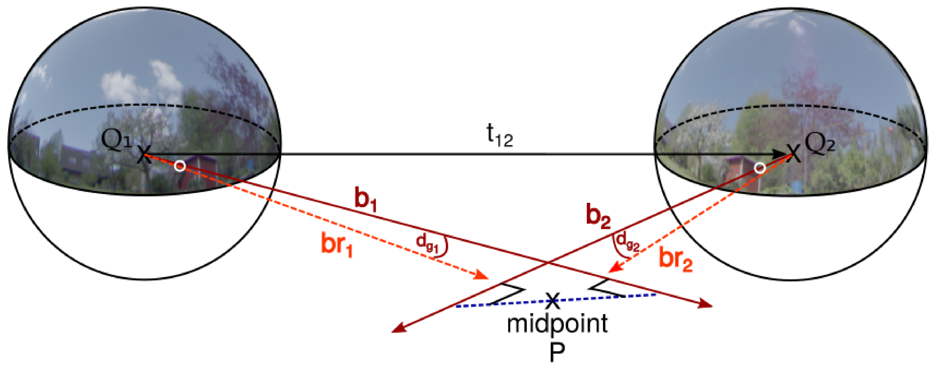
where is a measured bearing vector with unit length in one camera image and is the normalized reprojection of the triangulated world point from corresponding bearing vectors in both images. Geometrically, describes the arc length of the closest distance between two points on a unit sphere. For the triangulation of the three-dimensional world point, we use the mid-point method on calibrated camera rays. It finds the shortest line connecting the two rays and uses the mid-point of this segment as triangulated world point. We refer to [37] for a comprehensive review on triangulation methods and detailed descriptions. All of the computations for the evaluation are performed in world coordinates that are available based on the ground truth information saved for the datasets. Figure 4 shows the computation of the angular error.
The triangulated world point is computed by minimizing the squared distance of the two corresponding rays in both cameras:
Using the Moore-Penrose pseudoinverse , is found as . Here, is a matrix built of the bearing vectors and for both cameras respectively in world coordinates. The translation between camera positions and is . With , the triangulated world point is computed as . The reprojections to the cameras in world coordinates are given as for camera 1 and as for camera 2.
Following this approach for evaluation, we separately handle different special cases to improve the overall evaluation accuracy. The approach fails for bearing vectors that are parallel or antiparallel. For approximately parallel or antiparallel rays, small measurement errors or noise have a large effect. Therefore, we check for parallelism while using the constraint , where and are the bearing vectors and . If a pair of matched bearing vectors fulfills this constraint, then it is excluded from the evaluation. After triangulation of the world point, we check the orientation of the reprojections, which is equivalent to the cheirality constraint for perspective cameras. In the perspective camera case, the cheirality constraint checks that the reprojected points lie in front of the camera. For bearing vectors and with reprojections and , we use a generalized version and check whether and and classify the match as false, if one of the two conditions is not fulfilled [36].
The main condition that we use to classify a match as correct based on unit vectors and is
where combines the reprojection errors in both images and is set to 3°.
This condition also holds for features that lie within 3° to the epipolar curve, which is the equivalent to the epipolar line in perspective camera settings. These matches fulfill the epipolar constraint but can nevertheless be incorrectly matched. An example is shown in Figure 5. A part of these false matches can be detected by considering the assigned scale of these features from the detection in scale space and comparing the scales to the distances to the triangulated world point. This is related to the approach described in [38]. For the size of the feature regions and in image 1 and 2, respectively, and the corresponding distances and , we build the relations and and only accept features that fulfill the following condition:
This means that the scales of the features are required to be consistent with the distances to the triangulated world point, e.g., if the scale of feature A in image 1 is smaller than the scale of feature B in image 2, then the distance of the world point from camera 1 is required to be smaller than the distance of the world point from camera 2 and vice versa. We check this condition by evaluating the signs of the relations defined above. If the size of the features is equal (i.e. ), then we accept any relationship of the corresponding distances.
3.2. Datasets and Experimental Setup
The analysis of the inlier frequency curve is based on the ground-truth values available for the used datasets. The known positions and orientations of the camera images, together with the calibration parameters, enable the computation of the real transformations (translation and rotation) between two images and, thus, allow the analysis of the performance of the presented methods, as described in Section 3.1. For the computation of the inlier frequency curves, we build all possible image pairs within each dataset. For each image pair, we compute the inlier-frequency values for each method and then calculate the mean over all image pairs in one dataset. Additionally, we average over the mean values of all datasets.
For each keypoint detection method, we limit the number of detected keypoints to 1000, which is not always reached (e.g., due to low contrast regions). Additionally, for each method, we only consider the number of best matches that are available throughout all image pairs to allow for useful averaging. The differences in the number of available matches are mainly caused by the parallelism constraint that is described in Section 3.1.
For detailed information on the datasets, we refer to [39]. Summing up, we include four datasets of outdoor fisheye images and ground truth information. Two datasets are captured in a typical garden environment (Garden 1 and 2), one dataset is from a small parklike area (Finnbahn) and the fourth dataset is in the vicinity of the main building at Bielefeld University. The datasets include different illumination conditions, varying cloud coverage, and differing distances to visible features.
For the analysis of the inlier frequency curves, we used different parameter sets in the experiments. We tested varying values for the strength of the initial Gaussian filtering and different numbers of scale levels . We also performed experiments with masked sky regions to analyze the effect of misleading features in the sky region of the images. This way, keypoints that belong to clouds are neither detected nor matched.
4. Results
In this section, we present the results from experiments using the different available datasets. We show the results within and across datasets as well as exemplary results of single images, as the datasets bear particular challenges due to varying environments.
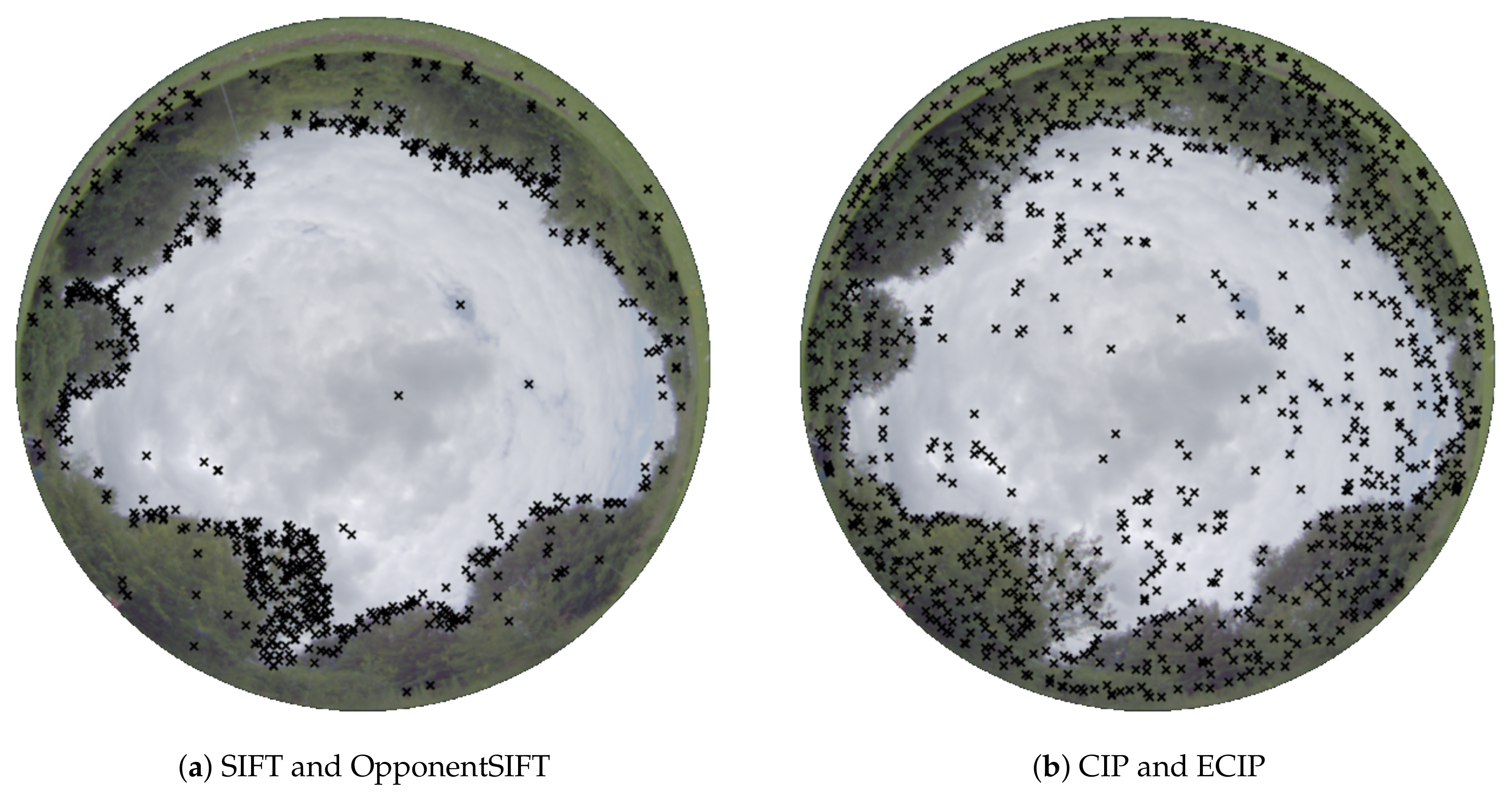
In Figure 6, two exemplary images from the dataset Finnbahn are shown with the most relevant 1000 keypoints detected by the different methods. On the left, keypoint positions from the grayscale method SIFT are plotted (OpponentSIFT uses the same keypoint positions). In contrast, the right plot shows the most relevant 1000 keypoints that were detected by CIP (also used for ECIP) with the detection done based on color information. The distribution of the keypoints show remarkable difference between both methods. When being limited to grayscale information, most features are detected on the transition from ground to sky, as this is the most prominent change in grayscale. Features within the ground region are less frequently detected and features in the cloudy sky are very rare. Conversely, CIP, which uses color information for the keypoint detection, detects features that are more uniformly distributed over the whole image. Interest points are selected within the ground region, as well as in the sky region; hence, they are not so concentrated on the skyline between ground and sky.
Exemplary images are shown in Figure 7 for the feature matching step. Here, the same image pair from the dataset Finnbahn is shown with the best 50 matches plotted for all four methods. The number of shown matches is restricted to 50 for this visualization. The color of the matches indicates the rank of each match, with darker colors corresponding to higher ranks. This ranking is computed by sorting the matches by their distance ratios. From top to bottom, the use of color information increases. The images are similarly oriented, such that most of the correct feature matches should be aligned horizontally. It can be seen that the number of correct matches increases with an increasing use of color information from top to bottom. For SIFT and OpponentSIFT high ranked as well as lower ranked matches show mismatches. For CIP and ECIP, the number of mismatches is smaller and, for ECIP, the mismatches come along with lower rankings.
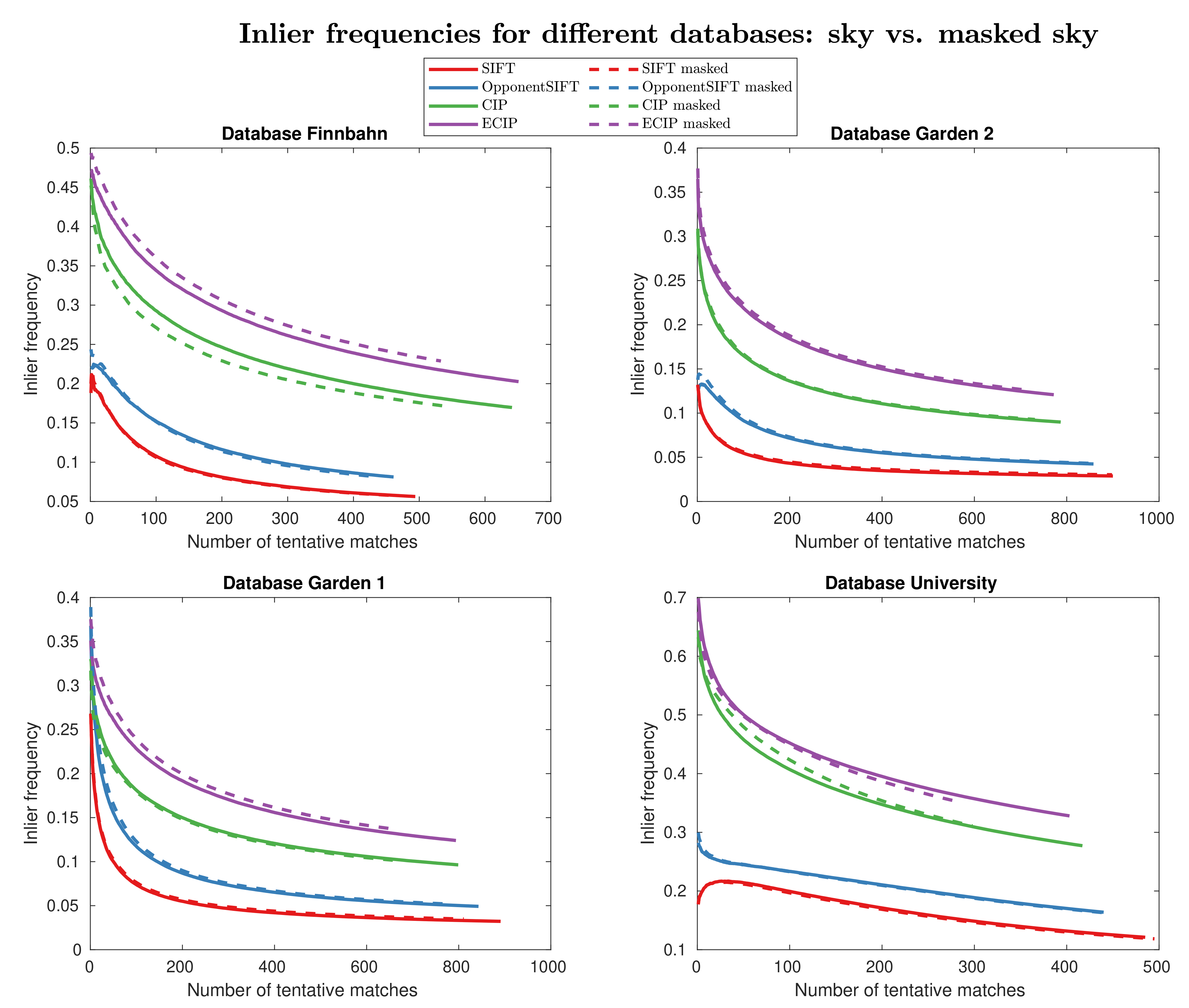
In Figure 8, the inlier frequency curves for the analyzed methods are shown for each dataset (, ). On the horizontal axis, the number of tentative matches are plotted, which are the found matches sorted with respect to the distance ratios. As described above, the number of tentative matches are clipped to the minimum available number of matches in each image pair within the datasets and thus vary across the different methods and datasets. As inlier frequencies are plotted on the vertical axis, higher values imply better performance. For all of the datasets, the ECIP method gives the highest values of inlier frequencies and SIFT yields the worst results. Overall, the increase in color information from SIFT to ECIP is reflected by a better performance of the methods. The largest improvement is found between OpponentSIFT and CIP. The results only reveal a minor impact of masking sky regions on the inlier frequency values.
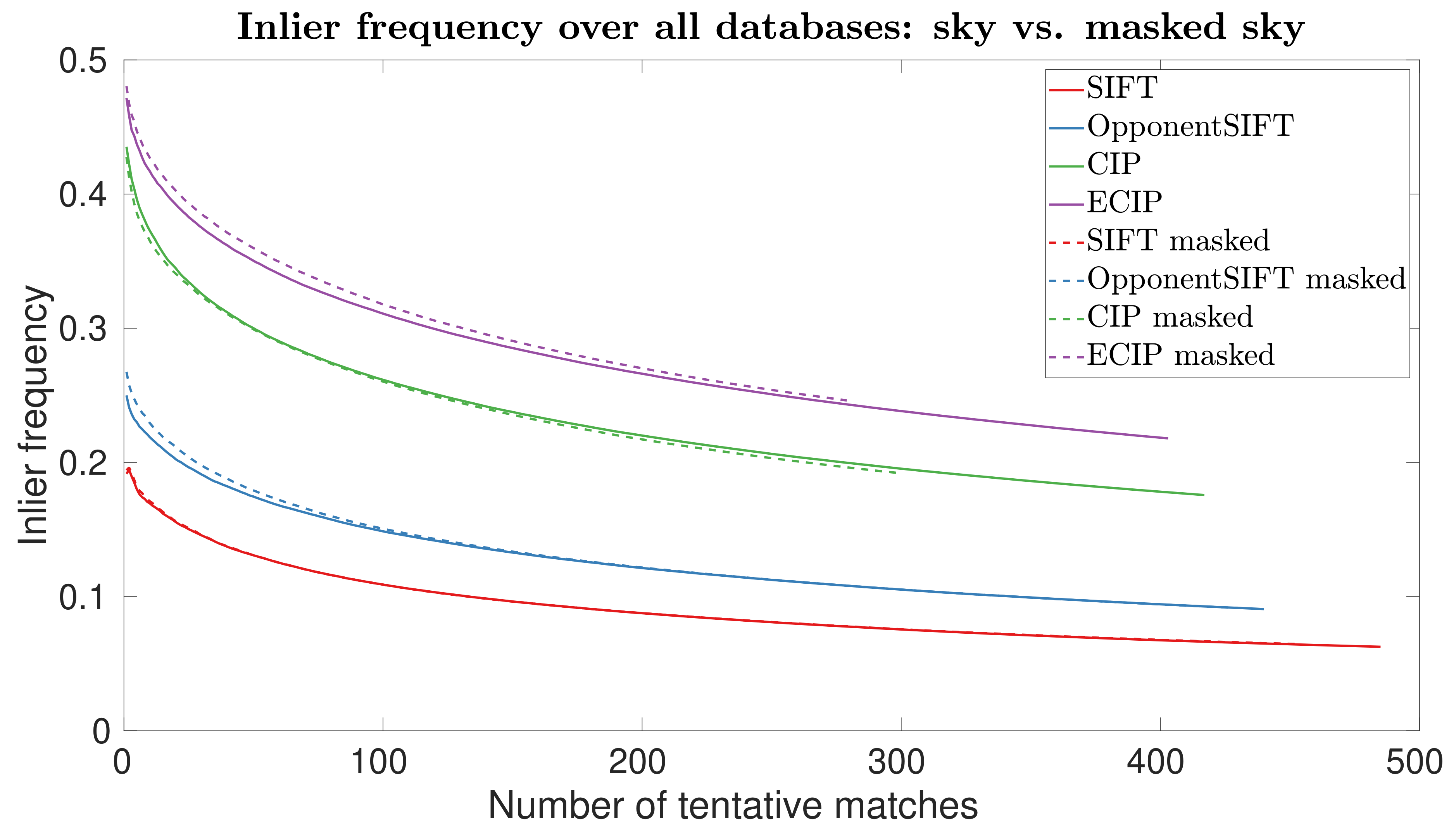
These results are also confirmed in Figure 9, which shows the inlier frequency curves from Figure 8 averaged over all four datasets. Summing up, the experiments show minor differences between grayscale or color descriptors. However, color detectors improve the performance considerably when compared to grayscale detectors. For color detectors, additional color information for the description step further improves the results. Masking of the sky regions to eliminate misleading features does not lead to markedly different results.
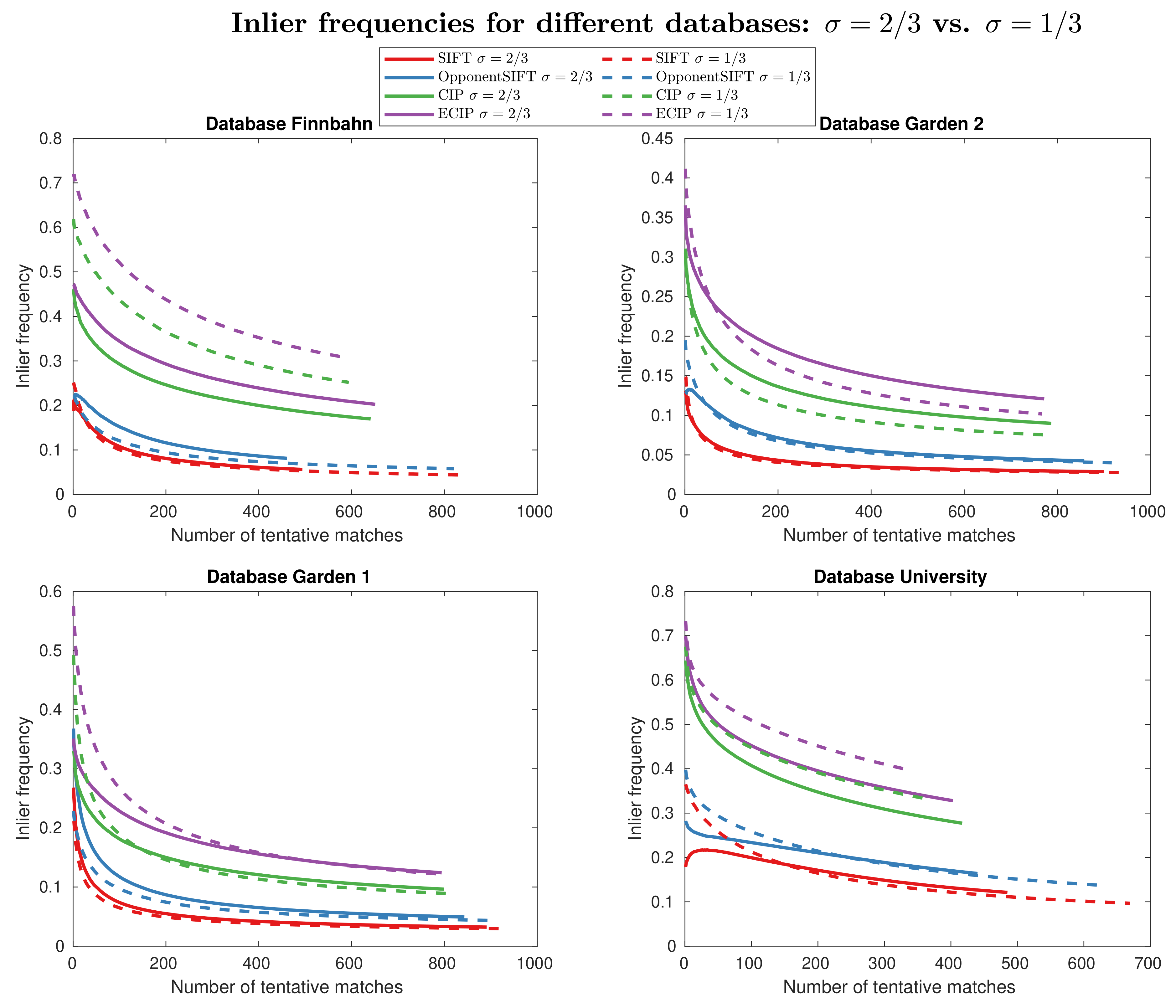
Figure 10 shows the effect of varying , which controls the strength of the Gaussian filtering. Here, strong differences across the datasets are visible. In the datasets Finnbahn and University, the smaller value of markedly improves the results for CIP and ECIP. In the dataset Garden 1, this effect is only apparent for small numbers of matches (< 300) and, in the dataset Garden 2, the inlier frequencies decrease, except for very small numbers of matches (< 50). For SIFT and OpponentSIFT, the effects are not so distinct, except for the dataset University, in which the use of improves the performance for small numbers of matches.
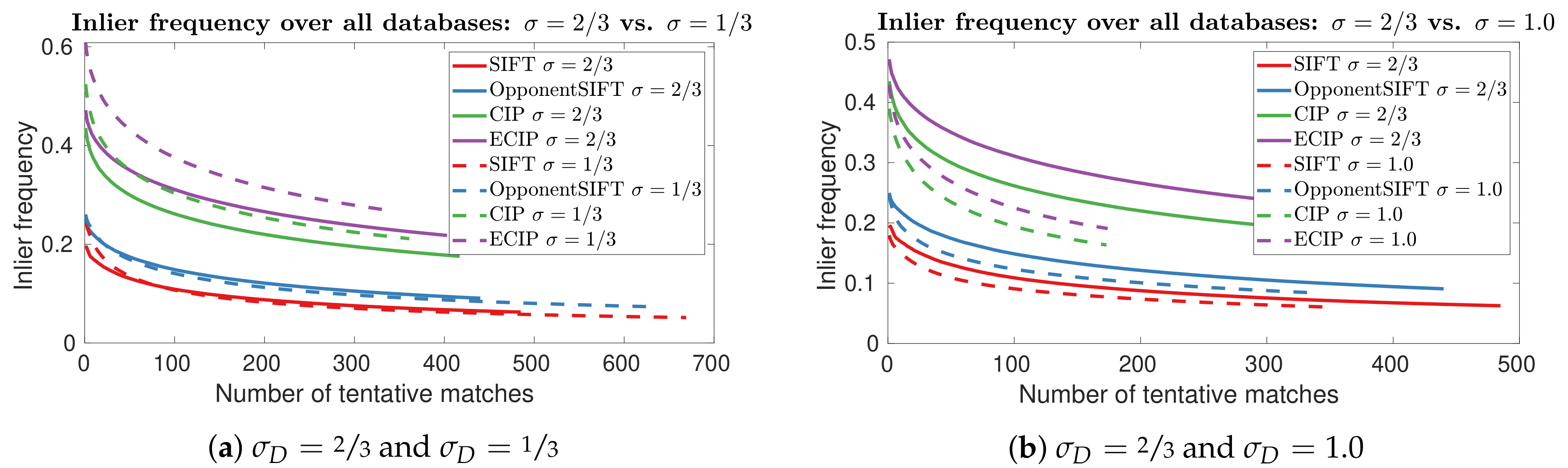
In Figure 11a, the results for and averaged over all datasets are plotted. For CIP and ECIP, the performance increases for smaller , whereas only minor differences are visible for SIFT and OpponentSIFT. The results for a higher value () are shown in Figure 11b, averaged over all the datasets. The plots for the individual datasets are omitted here, as they all show very similar results. It is visible that the increase of from to 1.0 leads to worse results for each method.
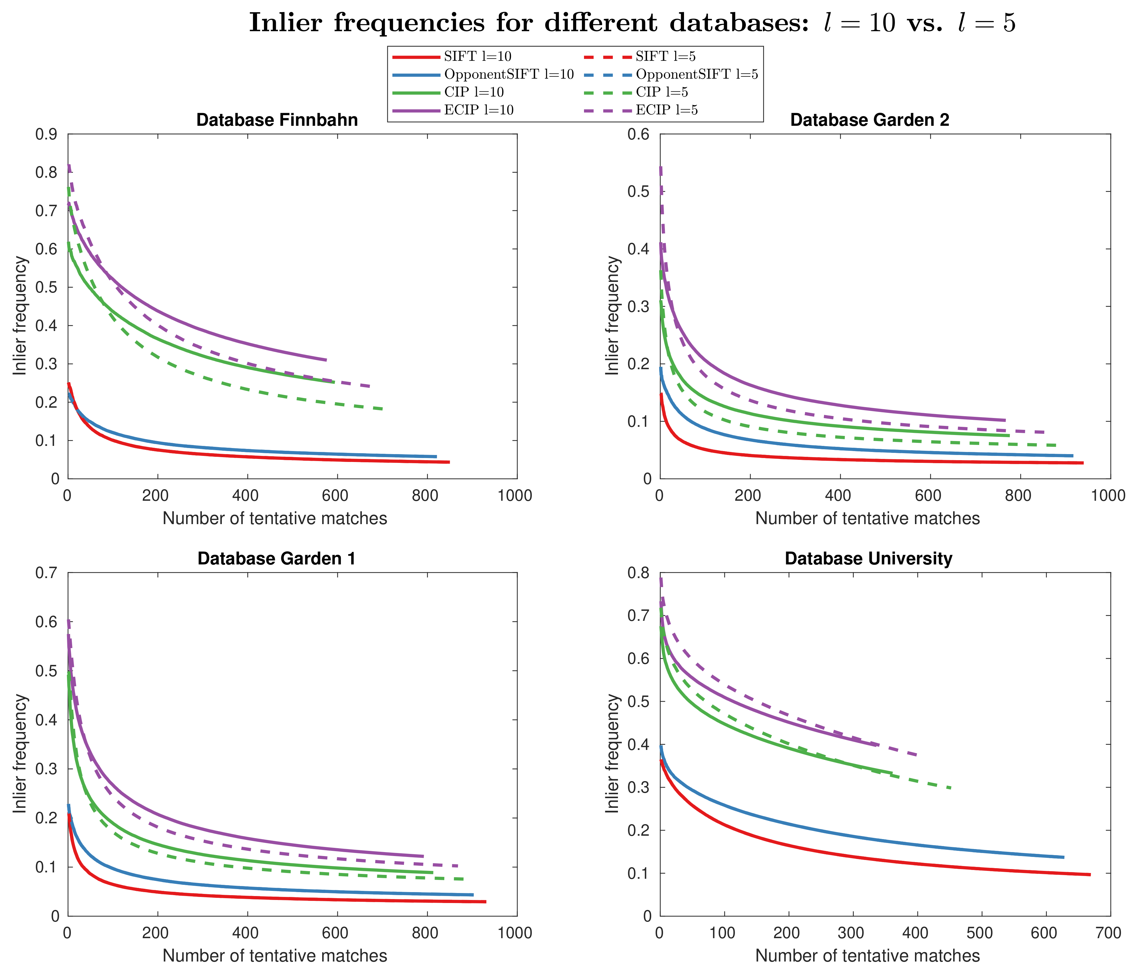
Another main parameter for CIP and ECIP is the number of layers used to compute the scale stacks. In Figure 12, the inlier frequency curves for the use of five and 10 layers are plotted ( is set to ). The results for SIFT and OpponentSIFT do not change, as the number of layers is differently defined and used in the OpenCV implementations and is therefore not varied within these experiments. The datasets Garden 1 and Garden 2 lead to similar results as the use of less layers () decreases the inlier frequencies. For the dataset Finnbahn, increased inlier frequency values appear for small number of matches, but, for higher number of matches. the results also get worse. In contrast are the results for the dataset University, in which results in slightly better values.
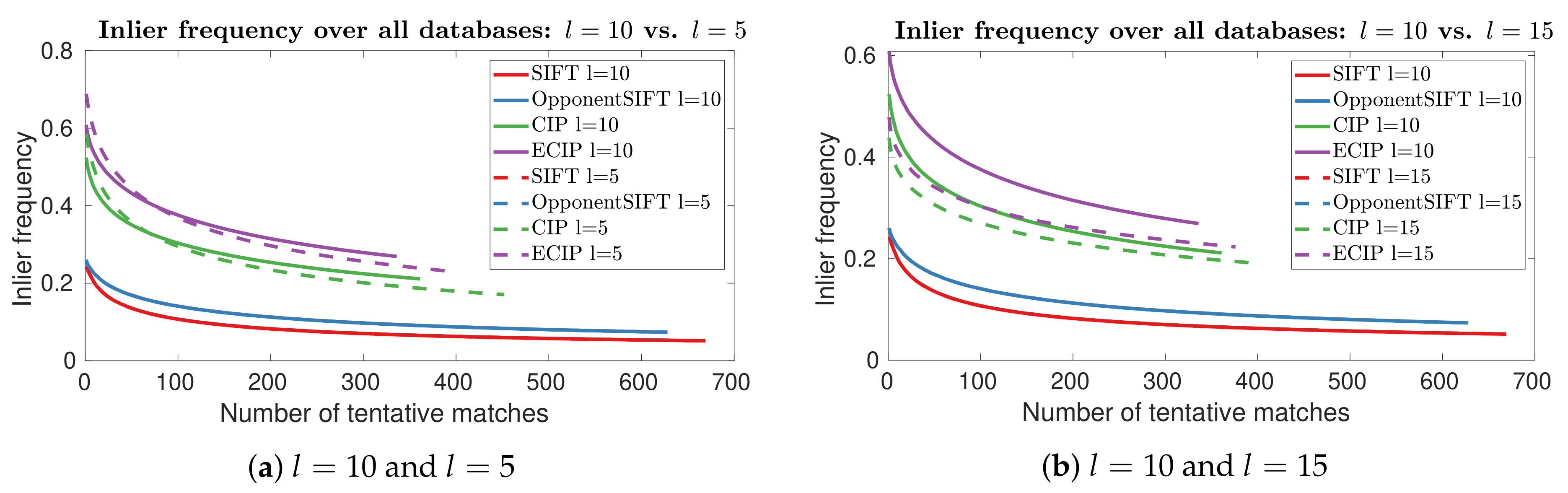
Averaged over all the datasets, we obtain improved results for approximately the first 100 matches, and worse results for higher amounts (see Figure 13a). The use of more layers () leads to lower inlier frequency values, regardless of the number of matches (Figure 13b).
Figure 14 shows a compact version in order to obtain an overview of the different results. For this, the inlier frequency value at is selected for each method and each parameter set, i.e., the value for the best 100 matches averaged over all datasets is extracted. The systematic labeling encodes the different parameter sets, where the token L is followed by the number of layers used and the token s is followed by the initial . Throughout all of the tested methods, ECIP with 10 layers and performs best. For each parameter combination, the ordering of the methods is the same, with SIFT leading to the lowest and ECIP resulting in the highest inlier frequencies. Equally high values for ECIP are reached with just five layers being used, which decreases the computational costs.
5. Discussion
The main result of the experiments is the improvement of performance going along with additional use of color information. The incorporation of color information leads to higher inlier-frequency values in all of the analyzed outdoor datasets. The best results are obtained if the color information is used in both the detection and description process. This increases the complexity of the feature detection and description, but it could make a subsequent RANSAC step feasible by providing acceptable inlier ratios and, thus, limiting the number of iterations needed. For our use case of solving relative-pose problems without feature tracking, the inlier ratio of the best analyzed method is still very low. However, the inclusion of color information leads to a strong improvement.
Regarding the masking of sky regions, our results only show minor differences. Even though the color detector apparently selects more interest points in the sky region (see Figure 6), the overall matching performance is higher yet. If more false matches occur in sky regions using color detectors, they do not outweigh the overall better matching performance. Figure 7 exemplarily shows that features in the sky region do barely appear within the best 50 matches. Therefore, mismatches in the sky (e.g., due to clouds) do not seem to cause a major problem for outdoor scenarios. This effect is different to the results of our previous study on sky masking in the context of the holistic MinWarping method [39], in which false information in the sky region markedly deteriorates the homing results. Moreover, this result is possibly limited to our datasets and specific use case which includes changes within a few hours, but not across multiple days or even seasons. In the context of stronger changes of illumination or appearance, e.g., across seasons, the performance of features in different regions of the images should be studied further. Various algorithms exist that use UV sensors to remove information in the sky region and focus on the skyline to enable robust visual navigation ([40,41]). In [42], Chen et al., propose a multi-scale attention learning system that supports the removal of sky regions by creating attention masks that actually filter out sky regions and focus on the ground regions of the images as salient regions.
The results concerning the initial suggest a smaller value for our datasets than that proposed in the original publications, which use ([24]). We reached the best results for , but the results show large differences among the datasets. In our datasets, most of the images contain small features representing objects far away from the camera accompanied by predominantly small baselines between camera positions. However, the datasets also comprise images with large features close to the camera and relatively large baselines due to our problem definition in Section 1. The choice of turns out to be appropriate for our datasets, but has to be chosen considering the characteristic of the images used. Similar relationships exist for the suitable number of layers which also depends on the underlying dataset. In addition to proposed in [24], we tested and . On average shows comparable results to , whereas leads to worse results. Besides the dependency on the dataset, the effect of l depends on the number of matches. For smaller number of matches (approximately less than 100), on average outperforms , but for a higher number of matches we see the opposite effect. Thus, the number of matches needed in the application should also be considered in the choice of l. However, better results for less layers () are only reached in the dataset University, in which most visible objects are far away from the camera and are subject to only small scale changes, as the baseline is mainly short in relation to the distances to the objects. For the other three datasets, which include closer objects, leads to better results. Thus, the choice of l is markedly dependent on the environment and a trade-off between performance and computational complexity.
6. Conclusions
Based on our experiments, we conclude that color information is a major aspect for improving the matching performance in outdoor environments. The additional information contained in color information can be used to reach inlier ratios that make subsequent navigation steps feasible. Further work is needed to analyze this effect in the context of relative-pose problems in combination with RANSAC. The increased computational complexity in the feature-detection and feature-description process has to be studied regarding the implications for subsequent RANSAC steps, as higher inlier ratios decrease the number of iterations needed in RANSAC and, thus, reduce the computational effort of this step.
Based on the presented results, using grayscale images only, the search space has to be limited, e.g., by tracking of features over time, which is not suitable for our application. However, the performed experiments show promising results for color detectors and descriptors. We focused on the one color method, but other grayscale detectors and descriptors could also benefit from extension to color information. A great number of grayscale detectors and descriptors exist with characteristics suitable for different datasets. An appropriate grayscale method could be used as a basis for a color extension. More research is needed in this context, before a particular color detector and descriptor can be recommended.
Concerning the use of fisheye images, particularly methods that consider the strong radial distortions are promising candidates. For example, Lourenco et al. [43] proposed modifications to SIFT that make it resilient to radial distortions. This method, called sRD-SIFT, could be used as a basis for a color detector and descriptor for outdoor applications with fisheye images.
Funding
This research received no external funding.
Acknowledgments
The author thanks Ralf Möller for fruitful discussions and helpful comments on the manuscript.
Conflicts of Interest
The author declares no conflict of interest.
Appendix A. Implementation Details of CIP
In this appendix, we describe our implementation of CIP in detail (see Section 2.3), which follows our understanding of [24]. To compute the scale stack of Harris energies, spatial first-order derivatives in x- and y-directions of the RGB-channels of the input image () are computed which are then transformed to the HSI-space. The derivatives in the HSI-space are computed from the individual derivatives in RGB-space using the equation from [27]:
Equation (A1) gives the spatial derivatives in the x-direction of the channels in the HSI-space with additional scaling of the derivative to account for the instabilities at the black-white axis at small values for saturation (for details see [44]). The derivatives in y-direction are computed analogously.
The first two components from Equation (A1), and , are the so-called shadow-shading-specular quasi-invariants and are used to compute the second-moment matrix M with different scale factors:
where x is the pixel location in the image, g is a Gaussian filter with the given standard deviation, is the differentiation scale, and is the integration scale with as in [24]. Here, ∗ denotes the convolution operator. From , the Harris energy for different scales can be computed by
We use as mentioned in [45]. Harris energy is computed for different scale levels s using , with and the factor .
To select a characteristic scale of a feature, the single-channel saliency image is computed and used for a Laplacian-of-Gaussian (LoG) on different scales as in [24]. The saliency image is built on the representation of the input image in HSI color space which is based on the opponent color space (Equation (1) in the main text):
As a preprocessing step, we shift the HSI channels separately to a mean of zero and normalize each channel by the standard deviation of the channel to get a normalized input matrix:
where is computed as
and and are computed in the same way. As we use fisheye images with pixels outside of the field of view set to 0, we exclude these pixels from the computations. From , the covariance matrix is build and the eigenvectors of are calculated using singular-value decomposition. The saliency image is the result of a scalar product of each three-dimensional pixel value at pixel index in space with the eigenvector which has the highest eigenvalue:
forms the basis for the computation of a modified LoG that additionally applies a circularly symmetric raised cosine kernel to achieve a stronger robustness to noise. This kernel is defined for each location as
The modified LoG is then calculated as
where and with * representing convolution and the Gaussian kernel with standard deviation . To compute the scale space of LoG, the same parameters as for the Harris energy scale space are used.
In the last step, the scale stack of Harris energies and the scale stack of the modified LoG are used to select interest points with their characteristic scales. In our implementation, potential interest points are searched in the Harris energy scale space as local maxima with respect to both scale and space which results in a search within 26 nearest neighbors (eight spatial neighbors and two adjacent scale levels). For these potential interest points, the characteristic scale level is selected as the scale level which maximizes the modified LoG with respect to scale. If more than one local maximum is found, the largest scale level is chosen, and if no local maximum is found, the interest point is discarded. The radius r of the corresponding size for a subsequent SIFT descriptor is computed as
Based on the positions of the interest points and their corresponding sizes, a standard SIFT descriptor [9] is computed on a grayscale image which is built by applying the standard conversion . For the computation of the SIFT descriptor, we use the implementation available in the openCV library.
References
- Mikolajczyk, K.; Schmid, C. A performance evaluation of local descriptors. IEEE Trans. Pattern Anal. Mach. Intell. 2005, 27, 1615–1630. [Google Scholar] [CrossRef] [Green Version]
- Van de Sande, K.; Gevers, T.; Snoek, C. Evaluating color descriptors for object and scene recognition. IEEE Trans. Pattern Anal. Mach. Intell. 2009, 32, 1582–1596. [Google Scholar] [CrossRef]
- Schmidt, A.; Kraft, M. The impact of the image feature detector and descriptor choice on visual SLAM accuracy. In Image Processing & Communications Challenges 6; Choraś, R.S., Ed.; Springer: Cham, Switzerland, 2015; pp. 203–210. [Google Scholar]
- Schmidt, A.; Kraft, M.; Kasiński, A. An evaluation of image feature detectors and descriptors for robot navigation. In International Conference on Computer Vision and Graphics; Springer: Berlin/Heidelberg, Germany, 2010; pp. 251–259. [Google Scholar]
- Gil, A.; Mozos, O.M.; Ballesta, M.; Reinoso, O. A comparative evaluation of interest point detectors and local descriptors for visual SLAM. Mach. Vis. Appl. 2010, 21, 905–920. [Google Scholar] [CrossRef] [Green Version]
- Schmidt, A.; Kraft, M.; Fularz, M.; Domagala, Z. Comparative assessment of point feature detectors and descriptors in the context of robot navigation. J. Autom. Mob. Rob. Intell. Syst. 2013, 7, 11–20. [Google Scholar]
- Barroso, T.M.; Ghita, O.; Whelan, P.F. Evaluating the performance and correlation of colour invariant local image feature detectors. In Proceedings of the 2014 IEEE International Conference on Image Processing (ICIP), Paris, France, 27–30 October 2014; pp. 5751–5755. [Google Scholar]
- Fischler, M.A.; Bolles, R.C. Random sample consensus: A paradigm for model fitting with applications to image analysis and automated cartography. Commun. ACM 1981, 24, 381–395. [Google Scholar] [CrossRef]
- Lowe, D.G. Distinctive image features from scale-invariant keypoints. Int. J. Comput. Vis. 2004, 60, 91–110. [Google Scholar] [CrossRef]
- Mathibela, B.; Posner, I.; Newman, P. A roadwork scene signature based on the opponent colour model. In Proceedings of the 2013 IEEE/RSJ International Conference on Intelligent Robots and Systems, Tokyo, Japan, 3–7 November 2013; pp. 4394–4400. [Google Scholar]
- Kirk, R.; Cielniak, G.; Mangan, M. L* a* b* Fruits: A Rapid and Robust Outdoor Fruit Detection System Combining Bio-Inspired Features with One-Stage Deep Learning Networks. Sensors 2020, 20, 275. [Google Scholar] [CrossRef] [Green Version]
- Dzulfahmi; Ohta, N. Performance evaluation of image feature detectors and descriptors for outdoor-scene visual navigation. In Proceedings of the 2013 2nd IAPR Asian Conference on Pattern Recognition, Naha, Japan, 5–8 November 2013; pp. 872–876. [Google Scholar]
- Krajník, T.; Cristóforis, P.; Kusumam, K.; Neubert, P.; Duckett, T. Image features for visual teach-and-repeat navigation in changing environments. Rob. Autom. Syst. 2017, 88, 127–141. [Google Scholar] [CrossRef] [Green Version]
- Valgren, C.; Lilienthal, A.J. SIFT, SURF & seasons: Appearance-based long-term localization in outdoor environments. Rob. Autom. Syst. 2010, 58, 149–156. [Google Scholar]
- Milford, M.; McKinnon, D.; Warren, M.; Wyeth, G.; Upcroft, B. Feature-based visual odometry and featureless place recognition for SLAM in 2.5 D environments. In Proceedings of the Australasian Conference on Robotics and Automation, Melbourne, Australia, 7–9 December 2011. [Google Scholar]
- Möller, R.; Krzykawski, M.; Gerstmayr-Hillen, L.; Horst, M.; Fleer, D.; de Jong, J. Cleaning robot navigation using panoramic views and particle clouds as landmarks. Rob. Autom. Syst. 2013, 61, 1415–1439. [Google Scholar] [CrossRef]
- Bai, X.; Wen, W.; Hsu, L.T. Using Sky-pointing fish-eye camera and LiDAR to aid GNSS single-point positioning in urban canyons. IET Intel. Transport Syst. 2020. [Google Scholar] [CrossRef]
- Hsu, L.T.; Tokura, H.; Kubo, N.; Gu, Y.; Kamijo, S. Multiple faulty GNSS measurement exclusion based on consistency check in urban canyons. IEEE Sens. J. 2017, 17, 1909–1917. [Google Scholar] [CrossRef] [Green Version]
- Ma, J.; Jiang, X.; Fan, A.; Jiang, J.; Yan, J. Image matching from handcrafted to deep features: A survey. Int. J. Comput. Vision 2020, 1–57. [Google Scholar] [CrossRef]
- Maffra, F.; Teixeira, L.; Chen, Z.; Chli, M. Real-time wide-baseline place recognition using depth completion. IEEE Rob. Autom Lett. 2019, 4, 1525–1532. [Google Scholar] [CrossRef]
- Kendall, A.; Cipolla, R. Geometric loss functions for camera pose regression with deep learning. In Proceedings of the IEEE Conference on Computer Vision and Pattern Recognition, Honolulu, HI, USA, 21–26 July 2017; pp. 5974–5983. [Google Scholar]
- McManus, C.; Churchill, W.; Maddern, W.; Stewart, A.D.; Newman, P. Shady dealings: Robust, long-term visual localisation using illumination invariance. In Proceedings of the 2014 IEEE International Conference on Robotics and Automation (ICRA), Hong Kong, China, 31 May–7 June 2014; pp. 901–906. [Google Scholar]
- Maddern, W.; Stewart, A.; McManus, C.; Upcroft, B.; Churchill, W.; Newman, P. Illumination invariant imaging: Applications in robust vision-based localisation, mapping and classification for autonomous vehicles. In Proceedings of the Visual Place Recognition in Changing Environments Workshop, IEEE International Conference on Robotics and Automation (ICRA), Hong Kong, China, 31 May–7 June 2014; Volume 2, p. 3. [Google Scholar]
- Stöttinger, J.; Hanbury, A.; Sebe, N.; Gevers, T. Sparse color interest points for image retrieval and object categorization. IEEE Trans. Image Process. 2012, 21, 2681–2692. [Google Scholar] [CrossRef] [Green Version]
- Barata, C.; Marques, J.S.; Rozeira, J. Evaluation of color based keypoints and features for the classification of melanomas using the bag-of-features model. In International Symposium on Visual Computing; Springer: Berlin/Heidelberg, Germany, 2013; pp. 40–49. [Google Scholar]
- Bradski, G. The OpenCV Library. 2000. Available online: https://www.drdobbs.com/open-source/the-opencv-library/184404319 (accessed on 29 July 2020).
- Gevers, T.; van de Weijer, J.; Stokman, H. Color feature detection. In Color Image Processing: Methods and Applications; Lukac, R., Plataniotis, K.N., Eds.; CRC Press: Boca Raton, FL, USA, 2006; Volume 9, pp. 203–226. [Google Scholar]
- Vigo, D.A.R.; Khan, F.S.; van de Weijer, J.; Gevers, T. The impact of color on bag-of-words based object recognition. In Proceedings of the 2010 20th International Conference on Pattern Recognition, Istanbul, Turkey, 23–26 August 2010; pp. 1549–1553. [Google Scholar]
- Leonardis, A.; Bischof, H. Robust recognition using eigenimages. Comput. Vis. Image Underst. 2000, 78, 99–118. [Google Scholar] [CrossRef]
- Saito, T.; Rehmsmeier, M. The precision-recall plot is more informative than the ROC plot when evaluating binary classifiers on imbalanced datasets. PLoS ONE 2015, 10, e0118432. [Google Scholar] [CrossRef] [Green Version]
- Olson, C.F.; Zhang, S. Keypoint recognition with histograms of normalized colors. In Proceedings of the 2016 13th Conference on Computer and Robot Vision (CRV), Victoria, BC, Canada, 1–3 June 2016; pp. 311–318. [Google Scholar]
- Mikolajczyk, K.; Schmid, C. Scale & affine invariant interest point detectors. Int. J. Comput. Vis. 2004, 60, 63–86. [Google Scholar]
- Schmid, C.; Mohr, R.; Bauckhage, C. Evaluation of interest point detectors. Int. J. Comput. Vis. 2000, 37, 151–172. [Google Scholar] [CrossRef] [Green Version]
- Chum, O.; Matas, J. Matching with PROSAC-progressive sample consensus. In Proceedings of the 2005 IEEE Computer Society Conference on Computer Vision and Pattern Recognition (CVPR’05), San Diego, CA, USA, 20–25 June 2005; Volume 1, pp. 220–226. [Google Scholar]
- Forssén, P.E.; Lowe, D.G. Shape descriptors for maximally stable extremal regions. In Proceedings of the 2007 IEEE 11th International Conference on Computer Vision, Rio de Janeiro, Brazil, 14–21 October 2007; pp. 1–8. [Google Scholar]
- Pagani, A.; Stricker, D. Structure from motion using full spherical panoramic cameras. In Proceedings of the 2011 IEEE International Conference on Computer Vision Workshops (ICCV Workshops), Barcelona, Spain, 6–13 November 2011; pp. 375–382. [Google Scholar]
- Hartley, R.I.; Sturm, P. Triangulation. Comput. Vis. Image Underst. 1997, 68, 146–157. [Google Scholar] [CrossRef]
- Churchill, D.; Vardy, A. Homing in scale space. In Proceedings of the 2008 IEEE/RSJ International Conference on Intelligent Robots and Systems, Nice, France, 22–26 September 2008; pp. 1307–1312. [Google Scholar]
- Hoffmann, A.; Möller, R. Cloud-Edge Suppression for Visual Outdoor Navigation. Robotics 2017, 6, 38. [Google Scholar] [CrossRef] [Green Version]
- Stone, T.; Mangan, M.; Ardin, P.; Webb, B. Sky segmentation with ultraviolet images can be used for navigation. In Proceedings of the 2014 Robotics: Science and Systems Conference, Berkeley, CA, USA, 12–16 July 2014. [Google Scholar]
- Stone, T.; Differt, D.; Milford, M.; Webb, B. Skyline-based localisation for aggressively manoeuvring robots using UV sensors and spherical harmonics. In Proceedings of the IEEE International Conference on Robotics and Automation (ICRA), Stockholm, Sweden, 16–21 May 2016; pp. 5615–5622. [Google Scholar]
- Chen, Z.; Liu, L.; Sa, I.; Ge, Z.; Chli, M. Learning context flexible attention model for long-term visual place recognition. IEEE Rob. Autom. Lett. 2018, 3, 4015–4022. [Google Scholar] [CrossRef] [Green Version]
- Lourenco, M.; Barreto, J.P.; Vasconcelos, F. sRD-SIFT: Keypoint detection and matching in images with radial distortion. IEEE Trans. Rob. 2012, 28, 752–760. [Google Scholar] [CrossRef]
- Van de Weijer, J.; Gevers, T.; Geusebroek, J.M. Color Edge Detection by Photometric Quasi-Invariants. In Proceedings of the Ninth IEEE International Conference on Computer Vision, Nice, France, 13–16 October 2003; pp. 1520–1525. [Google Scholar]
- Lindeberg, T. Image matching using generalized scale-space interest points. J. Math. Imaging Vis. 2015, 52, 3–36. [Google Scholar] [CrossRef] [Green Version]
Figure 1.
Visualization of feature detection and description approaches: (a) scale-invariant feature transform (SIFT) (b) OpponentSIFT.
Figure 1.
Visualization of feature detection and description approaches: (a) scale-invariant feature transform (SIFT) (b) OpponentSIFT.

Figure 2.
Computation of color interest points (CIP). (a) First phase: the computation of a Harris energy (HE) scale stack for a color input image is based on two color components and , for which spatial color gradients are computed in x and y directions (, , , and ). The HE-stack with scale parameter is used to detect a set of interest points by a maximum search. (b) Second phase: the selection of the characteristic scale s for the interest points detected in the first phase is based on a saliency image . The Laplacian of Gaussian operator with the scale parameter is applied to built the LoG-stack from which the characteristic scale s for each feature is selected.

Figure 3.
Visualization of feature detections: (a) color interest points (CIP); (b) extended color interest points (ECIP).
Figure 3.
Visualization of feature detections: (a) color interest points (CIP); (b) extended color interest points (ECIP).

Figure 4.
Schematic representation of the angular error used as inlier criterion. Feature vectors (, ) in the images taken at camera positions and are used to triangulate a world point of the features (midpoint ) and this world point is backprojected to the camera images to compute reprojection errors. and are the reprojections of the world point to the cameras and used to compute the geodesic reprojection errors and . The positions and orientations of the cameras in a world coordinate system are defined by the translation vector and rotation matrices.

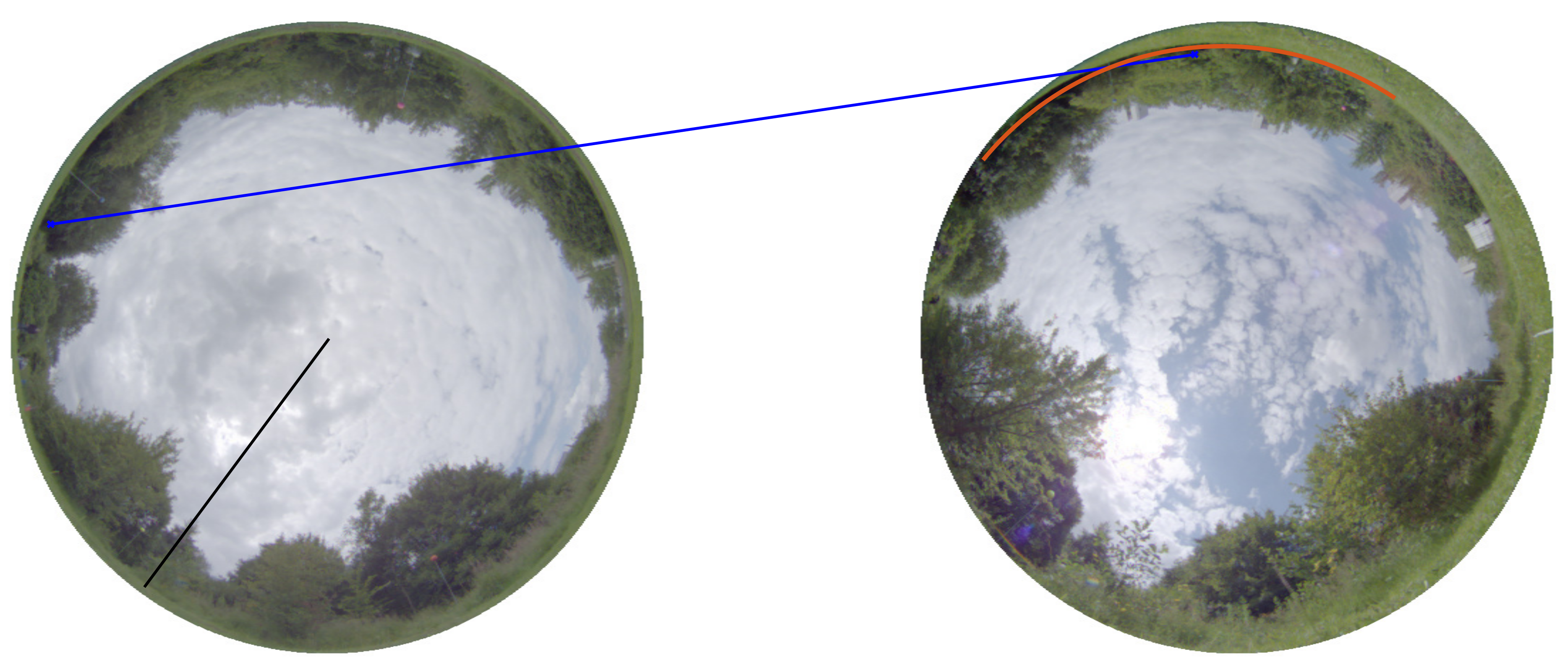
Figure 5.
Example of fulfilled epipolar constraint for wrongly matched features. The feature in the left image is not matched to the same feature in the right image. From the left camera position to the right camera position, a movement in the direction of the black line was executed. The blue line indicates a feature matching between the left and right features. Under the given movement vector, the feature in the left image moves along the epipolar curve of which a part is plotted in orange in the right camera image. As a consequence, the condition is fulfilled (here °).

Figure 6.
Different keypoint selections shown on one image: The most relevant 1000 key points are shown. (a) Keypoints based on grayscale information (used for SIFT and OpponentSIFT) (b) Keypoints based on color information (used for CIP and ECIP).
Figure 6.
Different keypoint selections shown on one image: The most relevant 1000 key points are shown. (a) Keypoints based on grayscale information (used for SIFT and OpponentSIFT) (b) Keypoints based on color information (used for CIP and ECIP).

Figure 7.
Examples of feature matches with different methods: From top to bottom the use of color information increases. For each method the best 50 matches, regarding their distance ratios, are shown. The color of the lines encodes the ranking of the matches, which is computed by sorting the matches by their distance ratios. The darker the color the higher ranked is the feature match.

Figure 8.
Inlier frequency curves for different datasets and different methods. For each dataset, the dashed lines show the results for masked sky regions, whereas the solid lines demonstrate the results based on the original input images.
Figure 8.
Inlier frequency curves for different datasets and different methods. For each dataset, the dashed lines show the results for masked sky regions, whereas the solid lines demonstrate the results based on the original input images.

Figure 9.
Inlier frequencies for original input images and masked sky regions as in Figure 8, but averaged over all datasets.
Figure 9.
Inlier frequencies for original input images and masked sky regions as in Figure 8, but averaged over all datasets.

Figure 10.
Inlier frequency curves for different datasets and different methods. For each dataset, the dashed lines show the results for , whereas the solid lines demonstrate the results for .
Figure 10.
Inlier frequency curves for different datasets and different methods. For each dataset, the dashed lines show the results for , whereas the solid lines demonstrate the results for .

Figure 11.
Inlier frequencies for varying averaged over all datasets.

Figure 12.
Inlier frequencies for different number of layers used in CIP and ECIP ( and ).

Figure 13.
Inlier frequencies for varying number of layers l averaged over all datasets.

Figure 14.
Inlier frequencies for different parameter sets. The inlier-frequency values at n = 100 are shown, i.e., the best 100 matches are considered.
Figure 14.
Inlier frequencies for different parameter sets. The inlier-frequency values at n = 100 are shown, i.e., the best 100 matches are considered.

© 2020 by the author. Licensee MDPI, Basel, Switzerland. This article is an open access article distributed under the terms and conditions of the Creative Commons Attribution (CC BY) license (http://creativecommons.org/licenses/by/4.0/).
Share and Cite
MDPI and ACS Style
Hoffmann, A. On the Benefits of Color Information for Feature Matching in Outdoor Environments. Robotics 2020, 9, 85. https://0-doi-org.brum.beds.ac.uk/10.3390/robotics9040085
AMA Style
Hoffmann A. On the Benefits of Color Information for Feature Matching in Outdoor Environments. Robotics. 2020; 9(4):85. https://0-doi-org.brum.beds.ac.uk/10.3390/robotics9040085
Chicago/Turabian StyleHoffmann, Annika. 2020. "On the Benefits of Color Information for Feature Matching in Outdoor Environments" Robotics 9, no. 4: 85. https://0-doi-org.brum.beds.ac.uk/10.3390/robotics9040085
Note that from the first issue of 2016, this journal uses article numbers instead of page numbers. See further details here.