One-Step Deadbeat Control of a 5-Link Biped Using Data-Driven Nonlinear Approximation of the Step-to-Step Dynamics

Abstract

For bipedal robots to walk over complex and constrained environments (e.g., narrow walkways, stepping stones), they have to meet precise control objectives of speed and foot placement at every single step. This control that achieves the objectives precisely at every step is known as one-step deadbeat control. The high dimensionality of bipedal systems and the under-actuation (number of joint exceeds the actuators) presents a formidable computational challenge to achieve real-time control. In this paper, we present a computationally efficient method for one-step deadbeat control and demonstrate it on a 5-link planar bipedal model with 1 degree of under-actuation. Our method uses computed torque control using the 4 actuated degrees of freedom to decouple and reduce the dimensionality of the stance phase dynamics to a single degree of freedom. This simplification ensures that the step-to-step dynamics are a single equation. Then using Monte Carlo sampling, we generate data for approximating the step-to-step dynamics followed by curve fitting using a control affine model and a Gaussian process error model. We use the control affine model to compute control inputs using feedback linearization and fine tune these using iterative learning control using the Gaussian process error enabling one-step deadbeat control. We demonstrate the approach in simulation in scenarios involving stabilization against perturbations, following a changing velocity reference, and precise foot placement. We conclude that computed torque control-based model reduction and sampling-based approximation of the step-to-step dynamics provides a computationally efficient approach for real-time one-step deadbeat control of complex bipedal systems.

1. Introduction

Since human personal and workspaces are built around the human form factor, we expect bipedal robots to be more suitable to integrate in homes, warehouses, and industry as compared to wheeled robots or quadrupedal robots. For bipedal robots to be practical they have to be able to: stabilize themselves when subject to exogenous disturbances (stability), accelerate quickly (agility), and move in complex terrain (versatility).

Controlling bipedal robots is a formidable challenge because of the following reasons. Bipedal robots are unstable due to the inverted pendulum-like dynamics, they have non-linear dynamics, they are under-actuated as there are more joints than there are actuators at the joints, and they are non-smooth due to changing contact dynamics. Although we can achieve control of non-linear, under-actuated systems such as the acrobot and the pendubot using large excursions of the links [1], the joint kinematic limits prevent such movements on the bipedal robots. In fact, bipedal systems are often instantaneously uncontrollable [2]. They cannot balance upright like an inverted pendulum because of limited ankle joint torques.

In this paper, we present a control technique that enables high fidelity control without being overly computationally heavy. We use partial feedback linearization to simplify control during the stance phase. This reduces the dynamics of the $N+1$ degrees of freedom planar robot with N actuated degrees of freedom to only 1 dimension. Thereafter, we exploit the fact that the step-to-step dynamics are a smooth function of the state and control, although the instantaneous dynamics are non-smooth, to approximate the step-to-step dynamics using Monte-Carlo simulations and non-linear regression. Finally, we use the one-dimensional step-to-step discrete equation for control without using computationally expensive non-linear optimization.

The most widely used approach is to use a simple model (e.g., linear inverted pendulum model) for control design and then map the simple model to the complex model using inverse kinematics [3]. Since the inverse kinematics model ignores the dynamics, these mapping technique works well for slow walking but not for fast walking. To realize faster, dynamic walking, one needs to use both the inverse kinematics and inverse dynamics to map from simple to complex models [4]. Another approach is the virtual model control which combines force control with inverse kinematics. In this method, one applies virtual forces at intuitively chosen locations (e.g., torso, foot) through components such as spring, dampers, dashpots, masses, latches, bearings, nonlinear potential and dissipative fields [5]. Then, one maps these forces to the joint torques using the appropriate Jacobian. Although the mapping is purely kinematic, it could generate controllers that enabled fast walking on the Spring Flamingo robot.

Nonlinear control may reduce complex dynamics to simpler linear dynamics. One popular approach is the virtual constraints approach [6,7]. Here, one slaves the actuated degrees of freedom to the un-actuated degrees of freedom, thus reducing the dimension of the robot to a mechanism with degrees of freedom equal to the un-actuated degrees of freedom. A similar approach is to use partial feedback linearization by inverting the mass matrix, Coriolis, centrifugal, and gravitation torques to decouple the un-actuated degrees of freedom from the actuated degrees of freedom [8,9]. Thereafter, one uses computed torque control or sliding mode control for trajectory tracking of the actuated degrees of freedom.

Since bipedal robots are almost impossible to control instantaneously due to under-actuation, they are best controlled over the time scale of step. One prominent idea is the use of capture point, which is the location the biped has to step to come to a complete stop [10]. A slightly more generalized approach is to use both the ankle push-off at foot-strike and foot placement to control the dynamics over the time scale of a step [11,12]. However, these methods use simple models of walking and need inverse kinematics and/or inverse dynamics to map to the full robot dynamics.

The virtual constraint method mentioned earlier affords asymptotic stability over a complete step [13]. The step-to-step stabilization, also known as orbital stabilization, is a dynamic measure of bipedal stability as compared to instantaneous or local stabilization [14]. More recent approaches formulate a control Lyapunov function approach within a virtual constraint framework that enables exponential local stabilization [15]. However, to improve orbital stabilization one can choose control parameters to minimize the biggest eigenvalue of the Jacobian of the step-to-step dynamics, which works well only for small perturbations [16]. Another method is to use event-based control where the linearization of the step-to-step dynamics is used to find control inputs to cancel the effect of small disturbances, but over the time scale of a step [17,18]. However, these linearized control methods can only provide stability for small perturbations.

Lyapunov functions provide a logical method for enabling controllers for large perturbations. Specifically, given a controller, one can compute a Lyapunov function and estimate the region of stability using sum-of-squares optimization provided the system can be approximated as a polynomial. One can then combine these regions of stability to find continuous controllers that stabilize the system from an initial condition to the reference motion using sampling-based methods such as rapidly exploring random trees [19]. Similarly, one can use the sum-of-squares optimization to compute a Lyapunov function certifying step-to-step or orbital stability [20,21]. Both the above methods find the region of stability for a given controller. Alternately, using a control Lyapunov function for orbital stability, one can find a controller and corresponding region of stability for a candidate Lyapunov function [22].

Deadbeat control refers to complete correction of disturbances/deviations in finite time [23]. Deadbeat control is unique to discrete-time systems as continuous-time control relying on proportional or proportional-derivative control can only achieve asymptotic convergence but not deadbeat convergence in finite time [24]. With legged systems, we are interested in one-step deadbeat control as this is important if the system has to meet tight constraints such as velocity tracking or stepping on a foothold. One method of achieving deadbeat control is to do a first order approximation in state and control of the step-to-step dynamics and use a discrete linear quadratic regulator, but this only achieves deadbeat control if the step-to-step dynamics are linear. For example, for the rimless wheel with a torso, the discrete linear quadratic regulator enables setting the torso angle once per step to achieve one-step deadbeat control [25]. For systems that demonstrate nonlinear step-to-step dynamics, one can use numerical root finding to find a deadbeat controller. For example, the step-to-step dynamics of the 3 dimensional spring-loaded inverted pendulum is non-linear and one can find foot placement angle and spring stiffness that enables two-step deadbeat control [26]. For more complex systems, simple models help compute control inputs to enable deadbeat control, and then map them to joint torques using inverse kinematics and/or inverse dynamics [27].

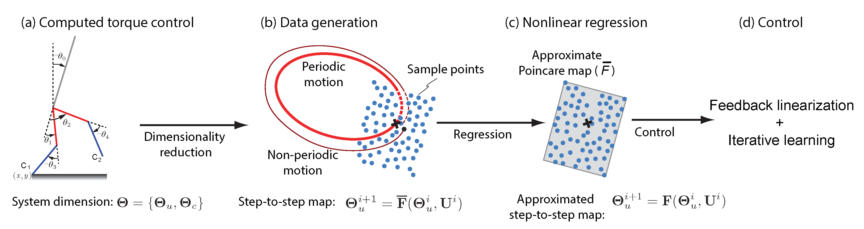
In this paper, we use computed torque control to reduce the dimensionality of the system from 10D to 2D (see Section 3.1). Thereafter, we use a data-driven approach to approximate the step-to-step dynamics with a simple model. Finally, this model is used for controller design. The use of a closed-form model of the step-to-step dynamics enables fast online control which is the main novelty of this work. Our earlier work demonstrated the approximation of the step-to-step dynamics for a simple model of running [28,29]. This paper extends our previous work in several ways as listed below and are the main contributions of this work.

• The use of computed torque control to reduce continuous dynamics to low degree of freedom system. Here, we reduce the state space in the single stance (continuous phase) from 10D to 2D.
• The use of Monte Carlo sampling followed by a low-order polynomial model and a high order error model to approximate the step-to-step map with relatively high accuracy. We represent the step-to-step map using a low dimensional control affine part comprising of a quadratic polynomial and high dimensional error term using Gaussian process model; the approximated model has about $98\%$ accuracy.
• Development of a computationally efficient method to find a one-step deadbeat controller. We use the control affine part to find the control inputs analytically, but then fine tune these control inputs using the Gaussian process error model using iterative learning that converges in less than 10 function evaluations.

A more comprehensive review of biped robots including modeling, design, control, and open problems may be found in these books [30,31].

2. Robot Model

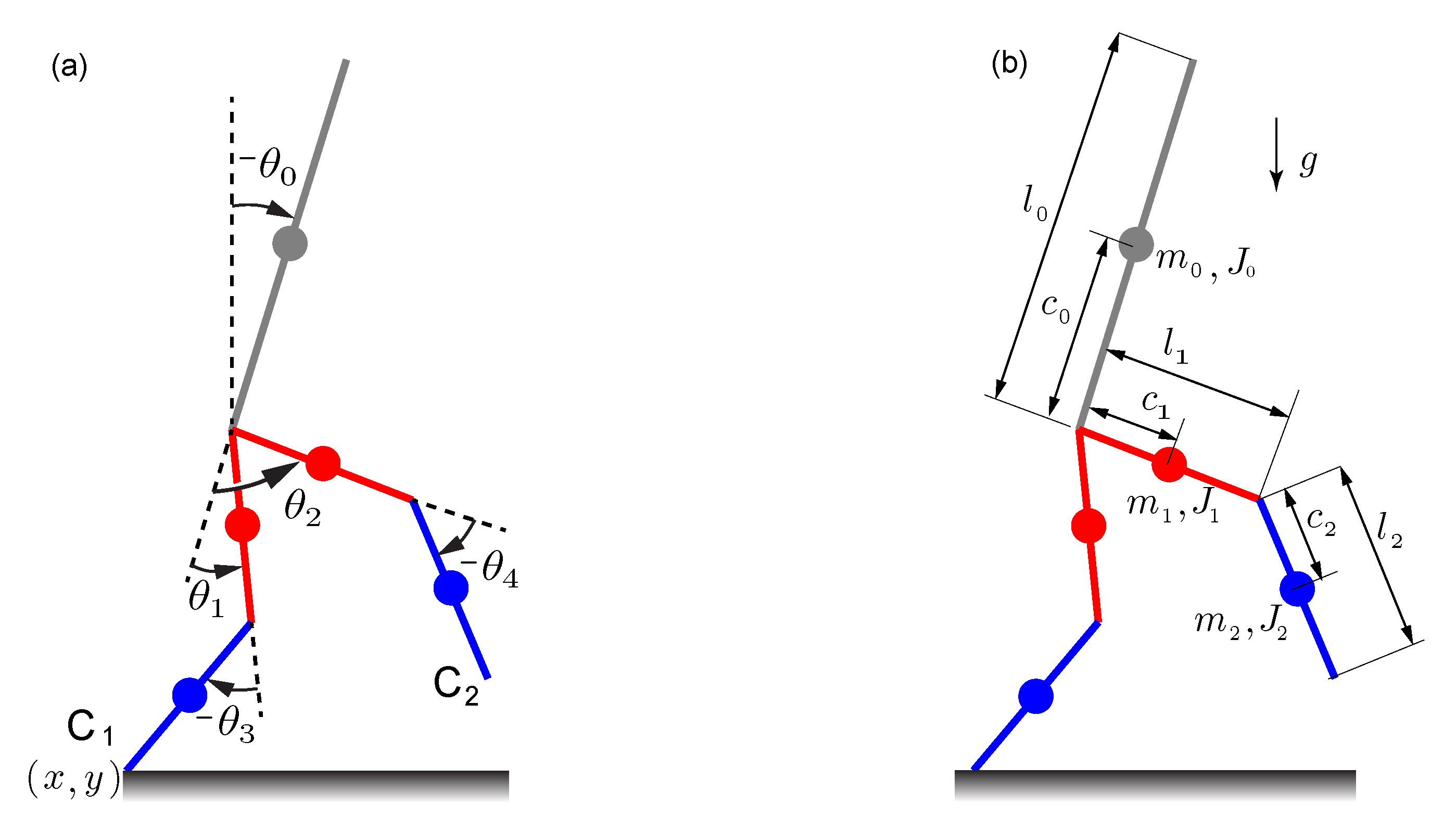
We show the 2D, 5-link model in Figure 1. We define the stance leg as the one that is in contact with the ground and the swing leg is the other leg. We show the configuration variables in Figure 1a. The foot in contact with the ground has coordinates $(x,y)$, where the x-axis is horizontal and y-axis is vertical. The torso angle ${\theta }_0$ is the angle between the torso and the vertical direction, ${\theta }_1$ and ${\theta }_2$ are the relative angles made by the thigh links of the stance and swing leg respectively with the torso, and ${\theta }_3$ and ${\theta }_4$ are the angles made by the calf links of the stance and swing leg respectively with their respective thigh links. We chose the mass, inertia, and length parameters to be similar to human morphology. The torso mass is $m_0=50$ kg, center of mass is at $c_0=0.5$ m, and inertia about the center of mass is $J_0=10$ kg·m${}^2$. The thigh links have a mass of $m_1=7$ kg, center of mass is at $c_1=0.25$ m, and inertia about the center of mass is $J_1=5$ kg·m${}^2$. The calf links have a mass of $m_2=5$ kg, center of mass at $c_2=0.25$ m, and inertia about the center of mass is $J_2=2$ kg·m${}^2$. Gravity points downwards and is $g=9.81$ m/s${}^2$. The torso length ${\ell }_0=1$ m the thigh link and calf link lengths are equal, ${\ell }_1={\ell }_2=0.5$.

There are two sets of equations which are derived using the Euler-Lagrange method [13]. One for the single stance phase where one foot is on the ground and second for the foot-strike where the legs exchange roles. We derive these next using the Euler-Lagrange method.

2.1. Single Stance Equations

The state variables are $\mathbf{q}=\left[\begin{array}{ccccccc}x& y& {\theta }_0& {\theta }_1& {\theta }_2& {\theta }_3& {\theta }_4\end{array}\right]$. The Lagrangian $\mathcal{L}=\mathcal{T}-\mathcal{V}=0.5\sum \left(m_i{v}_i^T{v}_i+J_i{\omega }_i^T{\omega }_i\right)-\sum \left(m_{i}g{y}_i\right)$, where $v_i$, ${\omega }_i$, $y_i$ are the linear velocity, angular velocity, and y-position center of mass of link i respectively. The summation is taken over all the 5 links. Using the Euler-Lagrange equations using $\mathbf{q}$ gives us 7 equations that may be compactly written as

$$\begin{array}{c}\hfill \mathbf{M}\left(\mathbf{q}\right)\ddot{\mathbf{q}}+\mathbf{C}(\mathbf{q},\dot{\mathbf{q}})\dot{\mathbf{q}}+\mathbf{G}\left(\mathbf{q}\right)=\mathbf{B}\mathbf{u}+{\mathbf{J}}_{C_1}{\mathbf{P}}_{C_1}\end{array}$$

(1)

where $\mathbf{M}$, $\mathbf{C}$, $\mathbf{G}$, $\mathbf{B}$ are the mass matrix, torques due to Coriolis and centrifugal acceleration, gravitational torque, and torque selection matrices. The control torques are $\mathbf{u}=\left[\begin{array}{cccc}{\tau }_1& {\tau }_2& {\tau }_3& {\tau }_4\end{array}\right]$, where ${\tau }_i$ is the torque for joint with degree of freedom ${\theta }_i$. ${\mathbf{J}}_{C_1}$ is the Jacobian from the stance leg contact point $C_1$ and ${\mathbf{P}}_{C_1}$ is the ground reaction force on the stance leg. Note that the top first two lines in Equation (1) are equivalent to change in linear momentum equals sum of external forces and remaining 5 are equivalent to change angular momentum equals external torques in the Newton-Euler formulation. Without loss of generality, we can assume $x=y=0$. Also, since $C_1$ is at rest, $\dot{x}=\dot{y}=\ddot{x}=\ddot{y}=0$. Using these conditions, we use the first two equations in Equation (1) to find the ground reaction forces ${\mathbf{P}}_{C_1}$ as a function of joint angles, velocities, and acceleration. We may write the remaining 5 equations as follows

$$\begin{array}{c}\hfill {\mathbf{M}}_{\theta }\left(\theta \right)\ddot{\theta }+{\mathbf{C}}_{\theta }(\theta ,\dot{\theta })\dot{\theta }+G_{\theta }\left(\theta \right)={\mathbf{B}}_{\theta }\mathbf{u}\end{array}$$

(2)

where ${\mathbf{M}}_{\theta }$, ${\mathbf{C}}_{\theta }$, ${\mathbf{G}}_{\theta }$, ${\mathbf{B}}_{\theta }$ are appropriately versions of the matrices defined earlier. We use this equation for simulating single stance phase and for controller development later.

2.2. Foot-Strike Equations

When the swing foot $C_2$ touches the ground, the single stance phase ends and the robot transitions to an instantaneous foot-strike. We also assume that the trailing leg applies an inline impulsive force ${\mathbf{I}}_{C_1}=I{\left[\begin{array}{cc}-sin({\theta }_0+{\theta }_1+{\theta }_3),& cos({\theta }_0+{\theta }_1+{\theta }_3)\end{array}\right]}^T$. This force comes from the ankle motor at $C_1$ which is passive during the stance phase, but applies an instantaneous impulse during take off (also see [32]). In this phase, angular momentum is conserved about new contact point $C_2$. We obtain the equations for this phase by integrating Equation (1) and taking the limit as time goes to 0 to get

$$\begin{array}{c}\hfill \left[\begin{array}{cc}\mathbf{M}\left({\mathbf{q}}^{-}\right)& -{\mathbf{J}}_{C_2}^T\\ {\mathbf{J}}_{C_2}& \mathbf{0}\end{array}\right]\left[\begin{array}{c}{\dot{\mathbf{q}}}^{+}\\ {\mathbf{I}}_{C_2}\end{array}\right]=\left[\begin{array}{c}\mathbf{M}\left({\mathbf{q}}^{-}\right){\dot{\mathbf{q}}}^{-}+{\mathbf{J}}_{C_1}^T{\mathbf{I}}_{C_1}\\ \mathbf{0}\end{array}\right]\end{array}$$

(3)

where the superscript − and + denote the instance before and after collision respectively.

2.3. Simulating a Single Step

We show the general equation that describes the motion of the system below. In the equation, we identified a single step as the repeating unit consisting of motion from one mid-stance to the next. We now explain the composition of a single step in the above equation. We start the step at mid-stance when stance leg thigh link is vertical given by ${\theta }_0+{\theta }_1=0$. There after we use the single stance Equation (2) to integrate the system till foot-strike. The foot strike occurs when the swing foot $C_2$ touches the ground and is given by $y_{C_2}={\ell }_{1}cos({\theta }_0+{\theta }_1)-{\ell }_{1}cos({\theta }_0+{\theta }_2)+{\ell }_{2}cos({\theta }_0+{\theta }_1+{\theta }_3)-{\ell }_{2}cos({\theta }_0+{\theta }_2+{\theta }_4)=0$. Thereafter we apply the foot strike condition given by Equation (3). Then we swap the legs using the following ${\theta }_0^{+}={\theta }_0^{-}$, ${\theta }_1^{+}={\theta }_2^{-}$, ${\theta }_2^{+}={\theta }_1^{-}$, ${\theta }_3^{+}={\theta }_4^{-}$, ${\theta }_4^{+}={\theta }_3^{-}$. Similarly, for the angular velocities we have ${\dot{\theta }}_0^{+}={\dot{\theta }}_0^{-}$, ${\dot{\theta }}_1^{+}={\dot{\theta }}_2^{-}$, ${\dot{\theta }}_2^{+}={\dot{\theta }}_1^{-}$, ${\dot{\theta }}_3^{+}={\dot{\theta }}_4^{-}$, ${\dot{\theta }}_4^{+}={\dot{\theta }}_3^{-}$. Thereafter we integrate the equations in single stance given by Equation (2) till the next mid-stance given by ${\theta }_0+{\theta }_1=0$.

3. Methods

3.1. Overview

We present an overview of our approach in Figure 2. As shown in Figure 2a, we use computed torque control to simplify the dynamics of the stance phase of a 5 link biped. This reduces the dimension from 10D to 2D. Thereafter, as shown in Figure 2b, we use a Poincaré map for modeling the step-to-step dynamics which further reduces the system dimension to 1D, the velocity of the stance leg. We note that the step-to-step dynamics has 1 state variable, the mid-stance speed, and 2 control variables, the push-off impulse and the step angle. As shown in Figure 2c, we approximate the step-to-step dynamics using a control affine model and Gaussian process model for the term not explained by the control affine part. Finally, as shown in Figure 2d, to find a deadbeat controller, we use the control affine model to find control inputs analytically using feedback linearization which is then fine tuned using the error model and iterative learning control.

3.2. Control in the Single Stance Phase Using Computed Torque Control

We show how to use computed torque control to control the actuated degrees of freedom in the stance phase. We invert the mass matrix from Equation (2) to get

$$\begin{array}{c}\hfill \ddot{\theta }={\mathbf{M}}_{\theta }^{-1}\left(\theta \right)({\mathbf{B}}_{\theta }\mathbf{u}-{\mathbf{C}}_{\theta }(\theta ,\dot{\theta })\dot{\theta }-{\mathbf{G}}_{\theta }\left(\theta \right))\end{array}$$

(4)

The system has 5 degrees of freedom, but only 4 actuators. We use partial feedback linearization to decouple the 4 degrees of freedom, namely the torso ${\theta }_0$, the swing leg joints ${\theta }_2$ and ${\theta }_4$, and the stance leg knee ${\theta }_3$. Thus, if ${\theta }_c=\left[\begin{array}{cccc}{\theta }_0& {\theta }_2& {\theta }_3& {\theta }_4\end{array}\right]$. Then, we can find a matrix ${\mathbf{S}}_c$ by inspection such that ${\theta }_c={\mathbf{S}}_c\theta$, where $\theta =\left[\begin{array}{cccccc}{\theta }_0& {\theta }_1& {\theta }_2& {\theta }_3& {\theta }_4& {\theta }_5\end{array}\right]$. We write

$$\begin{array}{c}\hfill {\ddot{\theta }}_c={\mathbf{S}}_c\ddot{\theta }={\mathbf{S}}_c{\mathbf{M}}_{\theta }^{-1}\left(\theta \right)({\mathbf{B}}_{\theta }\mathbf{u}-{\mathbf{C}}_{\theta }(\theta ,\dot{\theta })\dot{\theta }-{\mathbf{G}}_{\theta }\left(\theta \right))=\mathbf{v}\end{array}$$

(5)

where $\mathbf{v}$ is the new control input. We choose

$$\begin{array}{c}\hfill \mathbf{v}={\ddot{\theta }}_c^{\mathrm{ref}}+{\mathbf{K}}_{\mathbf{d}}({\dot{\theta }}_c^{\mathrm{ref}}-{\dot{\theta }}_c)+{\mathbf{K}}_{\mathbf{p}}({\theta }_c^{\mathrm{ref}}-{\theta }_c)\end{array}$$

(6)

where ${\theta }_c^{\mathrm{ref}}$, ${\dot{\theta }}_c^{\mathrm{ref}}$, ${\ddot{\theta }}_c^{\mathrm{ref}}$ are the user specified reference position, velocity, and acceleration. Here, we assume a fifth order polynomial for ${\theta }_c^{\mathrm{ref}}$ such that the position at the start and end are specified, velocity and acceleration at the start and end are 0. The gains ${\mathbf{K}}_{\mathbf{p}}$ and ${\mathbf{K}}_{\mathbf{d}}$ are diagonal matrices. We choose ${\mathbf{K}}_{\mathbf{p}}=K_{p}diag\{1,1,1,1\}$ and ${\mathbf{K}}_{\mathbf{d}}=2\sqrt{K_p}diag\{1,1,1,1\}$ to ensure critical damping in all the simulations. We can now get the motor torque as follows.

$$\begin{array}{c}\hfill \mathbf{u}={\left({\mathbf{S}}_c{\mathbf{M}}_{\theta }^{-1}\left(\theta \right){\mathbf{B}}_{\theta }\right)}^{-1}(\mathbf{v}+{\mathbf{S}}_c{\mathbf{M}}_{\theta }^{-1}\left(\theta \right)({\mathbf{C}}_{\theta }(\theta ,\dot{\theta })\dot{\theta }+{\mathbf{G}}_{\theta }\left(\theta \right)))\end{array}$$

(7)

The uncontrolled degree of freedom is ${\theta }_u={\mathbf{S}}_u\theta$, where ${\theta }_u={\theta }_1$. We can write an equation for this degree of freedom after suitably including the control input from the above equation

$$\begin{array}{c}\hfill {\ddot{\theta }}_u={\mathbf{S}}_u{\mathbf{M}}_{\theta }^{-1}\left(\theta \right)\left({\mathbf{B}}_{\theta }{\left({\mathbf{S}}_c{\mathbf{M}}_{\theta }^{-1}\left(\theta \right){\mathbf{B}}_{\theta }\right)}^{-1}\left(\mathbf{v}+{\mathbf{S}}_c{\mathbf{M}}_{\theta }^{-1}\left(\theta \right)({\mathbf{C}}_{\theta }(\theta ,\dot{\theta })\dot{\theta }+{\mathbf{G}}_{\theta }\left(\theta \right))\right)-{\mathbf{C}}_{\theta }(\theta ,\dot{\theta })\dot{\theta }-{\mathbf{G}}_{\theta }\left(\theta \right)\right)\end{array}$$

(8)

This is the only equation we need to integrate in the single stance phase.

3.3. Controlling the Step-to-Step Dynamics

We now introduce the idea of Poincaré section and map (see [33] for more details). The Poincaré section is a $2N-1$ (where N is the total degrees of freedom of the system) dimensional surface denoting an instance in the locomotion cycle (e.g., mid-stance, foot-strike). The Poincaré map is a function $\mathbf{F}$ that maps an initial state at the Poincaré section ${\mathsf{\Theta }}^i$ and controls during the step ${\mathbf{U}}^i$ to the state at the Poincaré section at the next step ${\mathsf{\Theta }}^{i+1}$. This map $\mathbf{F}$ describes the step-to-step dynamics and is found by integrating equations from mid-stance till foot-strike, then applying the algebraic equation for support transfer, and finally integrating the equations till the next mid-stance as shown in Figure 3. Thus, we can write

$$\begin{array}{c}\hfill {\mathsf{\Theta }}^{i+1}=\mathbf{F}({\mathsf{\Theta }}^i,{\mathbf{U}}^i)\end{array}$$

(9)

where i is the step number, $\mathsf{\Theta }=\left[\begin{array}{cc}\theta & \dot{\theta }\end{array}\right]$ is the state, where $\theta =\left[\begin{array}{cccccc}{\theta }_0& {\theta }_1& {\theta }_2& {\theta }_3& {\theta }_4& {\theta }_5\end{array}\right]$, $\mathbf{U}$ are the discrete controls that are set once per step (e.g., foot placement angle, impulsive push-off), and $\mathbf{F}$ is the Poincaré map that relates the state from one mid-stance to the next one. For most systems, it is not possible to find an analytical formula for the Poincaré map. It is obtained by numerically integrating the equations of motion and/or applying the algebraic conditions for instantaneous phases (e.g., footstrike). Note that we define the mid-stance as ${\theta }_0+{\theta }_1=0$. Therefore, for a 10 degree of freedom system, the Poincaré map is 9 dimensional.

We can simplify Equation (9) as follows. Assuming that the computed torque control works perfectly, the step-to-step dynamics only depend on the uncontrolled degrees of freedom, $\mathsf{\Theta }=\left[\begin{array}{cc}{\theta }_u& {\dot{\theta }}_u\end{array}\right]$ (Note, we show this in the results section). Thus, for the 5-link biped, we have ${\theta }_u={\theta }_1$. However, since the Poincaré map is at the mid-stance, there is only one degree of freedom, ${\dot{\theta }}_1$. We choose two controls to be the step angle at foot-strike ${\theta }_2=\alpha$ and the push-off impulse I at footstrike. Thus, we write

$$\begin{array}{cc}\hfill {}^m{\dot{\theta }}_1^{i+1}& =F{(}^m{\dot{\theta }}_1^i,{\alpha }^i,I^i)\hfill \end{array}$$

(10)

where ${}^m{\dot{\theta }}_1$ is the mid-stance speed of ${\theta }_1$. Also, note that F is a scalar.

3.4. Approximating the Step-to-Step Dynamics

We showed that the step-to-step dynamics reduces to a single equation, Equation (10). Thus, given the speed at mid-stance at step i, ${}^m{\dot{\theta }}_1^i$, we may use a combination of swing leg reference angle just before footstrike ${\alpha }^i$ and impulse $I^i$ to control the system. One caveat is that it is not possible to find an analytical solution to the step-to-step dynamics. Hence, we need to integrate the single stance equations and then apply the footstrike equation to obtain F numerically. However, for real-time control, it is best to get an analytical expression for F. In this section, we demonstrate a sampling-based method to approximate F.

First, we prepare the simulator to simulate a single step. The inputs are the mid-stance speed ${}^m{\dot{\theta }}_1^i$, the foot placement angle ${\alpha }^i$, and the push-off impulse $I^i$ and the output is the mid-stance speed at the next step ${}^m{\dot{\theta }}_1^{i+1}$. For some inputs, the simulator would lead to a failed state. We exclude these data points from the curve fitting.

Once we have a sufficient number of data points, we aim to curve fit the Poincaré map using a regression equation as given below

$$\begin{array}{cc}\hfill {}^m{\dot{\theta }}_1^{i+1}& =\overline{F}{(}^m{\dot{\theta }}_1^i,{\alpha }^i,I^i)\hfill \\ \hfill & ={\overline{F}}_{\mathrm{affine}}{(}^m{\dot{\theta }}_1^i,{\alpha }^i,I^i)+{\overline{F}}_{\mathrm{error}}{(}^m{\dot{\theta }}_1^i,{\alpha }^i,I^i)\hfill \\ \hfill & =f{(}^m{\dot{\theta }}_1^i)+g_1{(}^m{\dot{\theta }}_1^i){\alpha }^i+g_2{(}^m{\dot{\theta }}_1^i)I^i+{\overline{F}}_{\mathrm{error}}({\dot{\theta }}_i^m,{\alpha }^i,I^i)\hfill \end{array}$$

(11)

where $\overline{F}$ denotes the approximation of the Poincaré map which we split into two parts, a control affine part ${\overline{F}}_{\mathrm{affine}}$ and the error part that is not explained by the control affine representation, ${\overline{F}}_{\mathrm{error}}$. For the control-affine part, f, $g_1$, and $g_2$ are second order polynomials of the state ${}^m{\dot{\theta }}_1^i$. For the error part, ${\overline{F}}_{\mathrm{error}}$, we use Gaussian process regression model.

3.5. Feedback Linearization

The control problem is to track a reference mid-stance speed ${}^m{\dot{\theta }}_1^{\mathrm{ref}}$. Thus, given an initial state ${}^m{\dot{\theta }}_1^i{\ne }^m{\dot{\theta }}_1^{\mathrm{ref}}$, we need to find the controls ${\alpha }^i$ and $I^i$ such that the mid-stance speed at the next step is ${}^m{\dot{\theta }}_1^{i+1}=$ ${}^m{\dot{\theta }}_1^{\mathrm{ref}}$. Thus, effectively we aim to achieve complete correction and is known as one step deadbeat control [24,25].

There is only a single state variable to track ${}^m{\dot{\theta }}_1^{i+1}$ but there are two control inputs, $I^i$ and ${\alpha }^i$ (see Equation (10)). Thus, we have infinitely many solutions. We resolve this issue by using the two-one sided control approach as follows (also see [11]). If the mid-stance speed is greater than the reference speed then adjust the foot placement angle ${\alpha }^i$ but keep the push-off at the nominal value $I_0$. Similarly, if the mid-stance speed is slower than the reference speed then adjust the push-off impulse $I_0$ but keep the foot placement at the nominal value ${\alpha }_0$. The rationale behind two-one sided controllers is that push-off impulse is most effective to increase the speed and foot placement is most effective to reduce the speed.

To ensure rapid convergence to the reference motion, we need to have ${}^m{\dot{\theta }}_1^{i+1}=$${}^m{\dot{\theta }}_1^{\mathrm{ref}}$. Also note that mid-stance speed ${}^m{\dot{\theta }}_1^i$ is known as it is measured at mid-stance.

If ${}^m{\dot{\theta }}_1^i>{}^m{\dot{\theta }}_1^{\mathrm{ref}}$ then

$$\begin{array}{c}\hfill I^i=I_0,{\alpha }^i=\frac{-f{(}^m{\dot{\theta }}_1^i)-g_2{(}^m{\dot{\theta }}_1^i)I_0+{}^m{\dot{\theta }}_1^{\mathrm{ref}}}{g_1{(}^m{\dot{\theta }}_1^i)}\end{array}$$

(12)

If ${}^m{\dot{\theta }}_1^i<{}^m{\dot{\theta }}_1^{\mathrm{ref}}$ then

$$\begin{array}{c}\hfill {\alpha }^i={\alpha }_0,I^i=\frac{-f{(}^m{\dot{\theta }}_1^i)-g_1{(}^m{\dot{\theta }}_1^i){\alpha }_0+{}^m{\dot{\theta }}_1^{\mathrm{ref}}}{g_2{(}^m{\dot{\theta }}_1^i)}\end{array}$$

(13)

3.6. Stochastic Gradient Descent

The above feedback linearization control uses only the control affine model, which may not be completely accurate. After finding the control, ${\alpha }^i$ and $I^i$ we improve these controls using the $\overline{F}$ as follows. If ${}^m{\dot{\theta }}_1^i>{}^m{\dot{\theta }}_1^{\mathrm{ref}}$ then we refine the foot placement control

$$\begin{array}{c}\hfill {\alpha }_j^i={\alpha }_{j-1}^i+\lambda (\overline{F}-{}^m{\dot{\theta }}_1^{\mathrm{ref}})\end{array}$$

(14)

where j is the iteration number, $\lambda$ is a suitably defined constant (hand-tuned). If ${}^m{\dot{\theta }}_1^i<{}^m{\dot{\theta }}_1^{\mathrm{ref}}$ then we refine the push-off control

$$\begin{array}{c}\hfill I_j^i=I_{j-1}^i-\lambda (\overline{F}-{}^m{\dot{\theta }}_1^{\mathrm{ref}})\end{array}$$

(15)

We iterate the foot placement and push-off till we meet the following convergence criteria $(\overline{F}-{}^m{\dot{\theta }}_1^{\mathrm{ref}})<ϵ$, where $ϵ$ is a small user-defined number. We used $\lambda =0.5$ and $ϵ=0.001$. The stochastic gradient search converged in about 2 to 9 iterations in all results.

4. Results

4.1. Periodic Gait and Optimization Parameters

For the single stance controller, we divided the walking into two phases, mid-stance to foot-strike and foot-strike to mid-stance. In each of these phases we specify the reference position ${\theta }_c^{\mathrm{ref}}$, velocity ${\dot{\theta }}_c^{\mathrm{ref}}$, and accelerations ${\ddot{\theta }}_c^{\mathrm{ref}}$. We simplify by assuming a fifth order polynomial for each of these phases by specifying the position, velocity, and acceleration at the start and end. Since the reference ${\theta }_c^{\mathrm{ref}}$ has 4 references (${\theta }_0,{\theta }_2,{\theta }_3,{\theta }_4$), we have to specify 8 positions, 8 velocities, and 8 accelerations and 1 time for each phase. Thus, 25 constants per phase and since there are two phases (midstance to foostrike and foostrike to midstance), we have 50 constants per step.

We simplify this assignment as follows. For the mid-stance to footstrike, we set all initial and final velocities and accelerations to zero. We set the position at the start to the current location of the joints, all the end positions to zero except the swing calf angle which we set to ${\theta }_4=-0.5$ to allow for foot clearance during leg swing. We set the time to $0.2$ s assuming that this phase is longer than $0.2$ s. For the footstrike to midstance phase, we again set all initial and final velocities and accelerations to zero. We set the position at the start to the current position of the joints, all the end positions except the swing thigh angle which we set to ${\theta }_2={\alpha }_0=0.375$. We also set the time to $0.2$ s. We set the nominal push-off impulse of $I_0=0.18M\sqrt{gL}$, where $0.18$ is the non-dimensional impulse, $M=(m_0+2m_1+2m_2)$ and $L={\ell }_1+{\ell }_2$. Also, we use $K_p=100$.

We use MATLAB to create a simulation of a single step using the description in Section 2.3 and using Equations (2) and (3). Next, to find a periodic gait for the given control parameters ${\mathbf{U}}_0$, we solve the following equation for ${\mathsf{\Theta }}_0$ (see [34] for more information).

$$\begin{array}{c}\hfill {\mathsf{\Theta }}_0=\mathbf{F}({\mathsf{\Theta }}_0,{\mathbf{U}}_0)\end{array}$$

(16)

Using numerical integration with $\mathit{ode}\mathit{113}$ we obtain ${\mathsf{\Theta }}_0=\left[\begin{array}{cccccccccc}0& 0& 0& -1.0928& 0& 0& 0& 0& -0.5& 0\end{array}\right]$. This nominal gait corresponds to a speed of $1.27$ m/s, step time of $0.58$ s, and step length of $0.73$ and is similar to human cadence [35,36].

Next, we use central difference to find the Jacobian of Poincaré map $\frac{\partial F}{\partial \mathsf{\Theta }}$. Then we find the eigenvalues to establish the stability of the system. Only one eigenvalue is non-zero and is equal to $0.75$. Having all eigenvalues at zero except one implies that the step-to-step map is only one-dimensional. Since the only nonzero eigenvalue is less than 1, the system is stable for small perturbations [33]. Thus, the step-to-step map is 1D and the goal of the modeling and control mentioned in the ensuring sections is to nullify the uncontrolled degree of freedom over the time scale of a step.

4.2. Data Generation for the Step-to-Step Map and Curve Fitting

In our MATLAB simulation of a single step, we incorporate falling detection that includes conditions under which we terminate the simulation. These conditions include: (1) leg stubbing during swing phase, (2) swing times is shorter than $0.2$ s, (3) falling backwards by noting the speed at mid-stance, (4) hip inside the ground, and (5) flight phase when the ground reaction forces is zero.

To generate data, our inputs are in the range $-1.5\le {}^m{\dot{\theta }}_1^i\le -0.7$, $0.2\le {\alpha }^i\le 0.6$ and $0\le I^i\le M\sqrt{gL}$ using increments of $0.05$. Then using the single step simulation to generate the output ${}^m{\dot{\theta }}_1^{i+1}$. The total input had 891 data points (${}^m{\dot{\theta }}_1^i,{\alpha }^i,I^i$), out of which 649 led to a failed step and 242 gave us valid mid-stance speed ${}^m{\dot{\theta }}_1^{i+1}$. We used $75\%$ or 186 of the valid data points for training and the remaining $25\%$ or 56 for testing the fit.

To fit the data, we first used quadratic polynomials in ${}^m{\dot{\theta }}_1^i$ for the function f, $g_1$ and $g_2$ in ${\overline{F}}_{\mathrm{affine}}$ (see Equation (11)). For example, $f=a_0+a_1^m{\dot{\theta }}_1^i+a_2{{(}^m{\dot{\theta }}_1^i)}^2$, where $a_0$, $a_1$, and $a_2$ are constants found from regression by minimizing the squared error between the model and the data. We then checked if the affine part ${\overline{F}}_{\mathrm{affine}}$ is a good fit for the data. We found that $87\%$ of the test data was within $90\%$ accuracy and $98\%$ of the data was within $80\%$ accuracy. Next, we curve fitted the error using ${\overline{F}}_{\mathrm{error}}$. We used Gaussian process regression with a constant basis and it resulted in fitting $100\%$ of the data within $98\%$ accuracy.

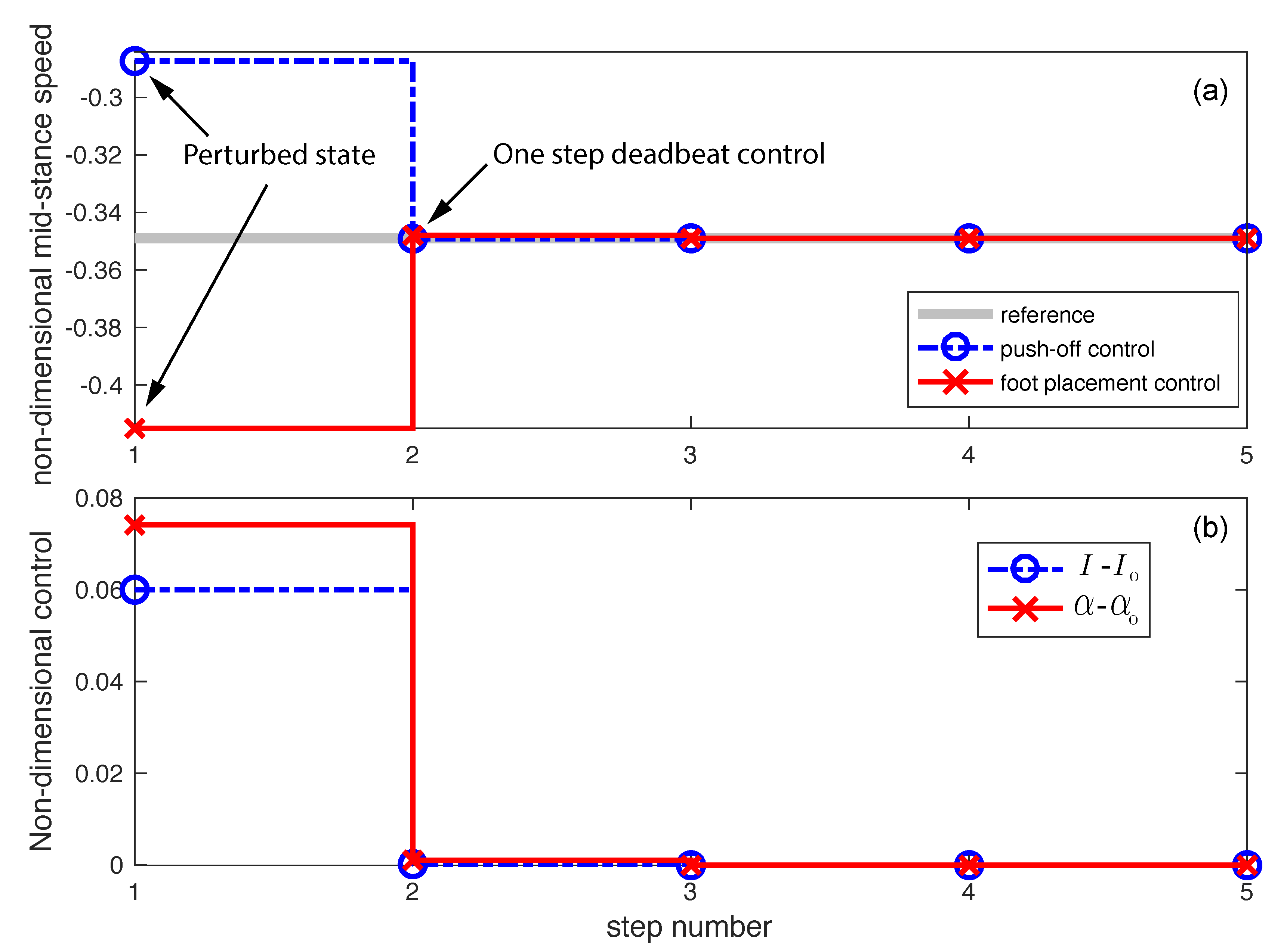
4.3. Stability

Stability is the ability of the system to correct deviation in the state from the nominal state. These deviations could come from exogenous disturbances to the system. The nominal state is ${}^m{\dot{\theta }}_1^{\mathrm{ref}}=-1.092$ rad/s. We imposed two different perturbations on the system and ran the simulations. In our first perturbation, we slowed the system to ${}^m{\dot{\theta }}_1^i=-0.9$ rad/s and second one we speed up the system to ${}^m{\dot{\theta }}_1^i=-1.3$ rad/s. We then controlled the system for each of these perturbations. The results are shown in Figure 4. In Figure 4a shows the mid-stance speed normalized against nominal speed ${}^m{\dot{\theta }}_1^{\mathrm{ref}}$ and (b) shows the control used subtracted from the nominal control values, both as a function of steps. As discussed earlier, the controller modulates the push-off control to speed up the system (red solid line) and modulates the foot placement to slow down the system (blue dashed line) to the reference speed. In both cases, it takes only one step to get to the nominal speed or onestep deadbeat control.

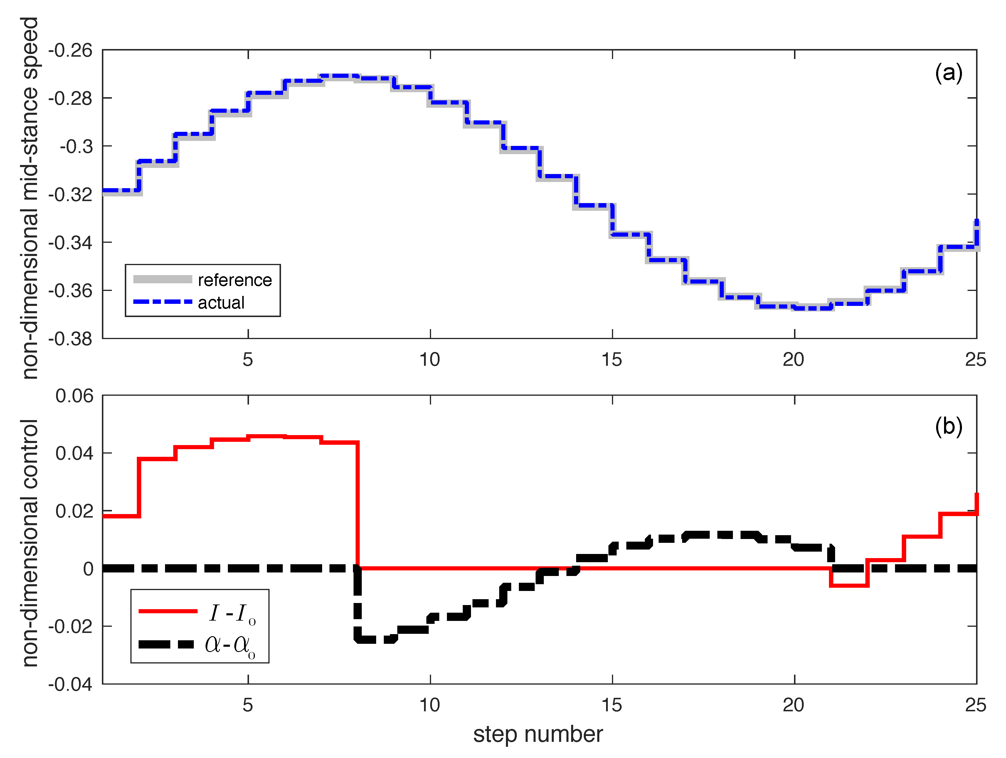
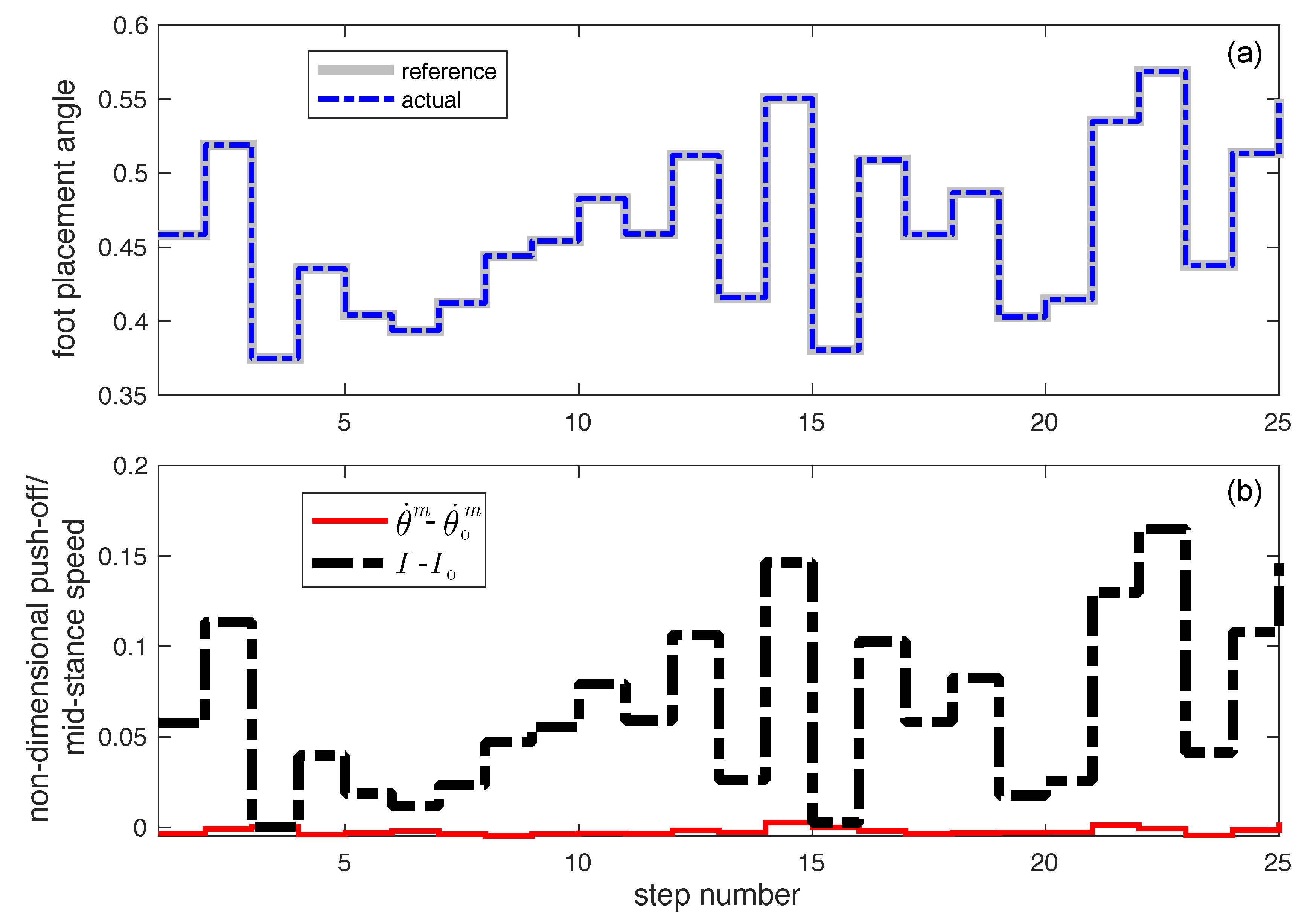
4.4. Agility

Agility is the ability of the system to rapidly change its speed and/or direction [37]. Here we consider the ability to change its speed by specifying a sinusoidally varying reference speed that changes at every step for 25 steps as shown in Figure 5a. The controller can track this reference with negligible error. We show the control in Figure 5b, where we have shown the net change in control with respect to the nominal control values. In a nutshell, the push-off controller is used to speed up the system and foot-placement control is used to reduce the speed.

4.5. Versatility

Versatility is the robot’s ability to perform a variety of tasks such as walking, standing, turning, climbing stairs [38]. Here we restrict to the specific task of walking over stepping stones. We can formulate this by specifying footstep locations or fixing the foot placement angle at every step. We generated 25 random foot placement positions from $0.375$ to $0.575$ rad. We fixed the foot placement angle to these values and specified the mid-stance speed to be the nominal speed ${}^m{\dot{\theta }}_1^{\mathrm{ref}}=-1.092$ rad/s. Here, we remove the restriction on the one-sided control and allowed the push-off to vary (decrease/increase) as specified by Equations (13) and (15). Figure 6a shows the foot placement angles (constraints) and Figure 6b red solid line shows the mid-stance speed subtracted from the nominal value and is zero indicating the tracking is perfect. The black dashed line in Figure 6b shows the push-off control used to achieve balance stability while achieving foot placement and velocity regulation.

5. Discussion

We demonstrated that by using computed torque control we can reduce the step-to-step dynamics of a 5 degrees of freedom model with a 10 dimensional state space to only 1 dimension. Next, we showed that using Monte-Carlo sampling and forward simulations, we can approximate the 1-dimensional step-to-step dynamics with about $80\%$ accuracy using a control affine model, but with $98\%$ accuracy when we supplement the control affine model with a Gaussian process model. Finally, we demonstrated that the control affine model enabled the analytical solution for the control input which we then fine tuned in 2 to 9 iterations using the Gaussian process model to enable perfect tracking or one-step deadbeat control.

We used computed torque control, a feedback linearization technique, to reduce the dimension of the continuous dynamics from 10 dimensions to 2 dimensions. The resulting feedback linearization is simple, but since it relies on canceling the natural dynamics, the Coriolis, the centrifugal, and gravitational torques, it is not necessarily energy efficient. Another method for feedback linearization is the method of virtual constraints where one controls the actuated degrees of freedom to follow the unactuated degrees of freedom, thus reducing the system dimension to the unactuated degrees of freedom [6]. The major difference between computed torque control and virtual constraints is that while computed torque control allows actuated degrees of freedom to be controlled independent of each other, the method of virtual constraints does not. Since the actuated degrees of freedom are independent, we may modify them in real time without affecting the step-to-step dynamics. One situation where this is useful is when we need to modify the reference motion to increase the foot clearance during swing. On the other hand, one needs to choose the virtual constraints prior to start of leg swing to avoid scuffing.

One-step deadbeat control is important for bipedal robots to go into environments that pose strict constraints (e.g., foot holds, narrow edges). Since these constraints are imposed over the time scale of a step and the system dynamics are non linear, it is often the case to integrate these equations of motion repeatedly over the time scale of a step to find the control inputs. Here, we simplify finding the deadbeat control strategy by: one, using partial feedback linearization to reduce the dimension of the step-to-step dynamics, and two, approximating the resulting low-dimensional step-to-step dynamics with an analytical control affine model and a Gaussian process model for the error term. The latter enables us to use the control affine model to find an analytical solution for the control input which is then fine-tuned with the Gaussian process error model. The fine tuning takes only about 2 to 9 iterations. The relatively low computational requirements of the method would potentially enable online computation of control inputs.

The under-actuation of walking robots combined with the weak coupling between the swing leg and the torso leads to a significant control problem. Another robot example with these features is the acrobat [39], a two link pendulum but with a single actuator. In the case of the acrobat, one can stabilize the system by using the unrestricted swinging motion of its actuated link, thus relying on the dynamic coupling. However, the swing leg angles and speeds are severely restricted in walking robots, thus strategies that have worked for acrobat are unusable for walking robots. With walking robots, the step-to-step motion dynamics, particularly managing energy exchanges because of foot collision and push-off, offer a powerful means of control [40], which we exploit.

The step-to-step controls offer four significant benefits. One is that the step-to-step dynamics are a smooth function of state and control, and thus one may use control techniques that have worked on smooth systems. Two, the step-to-step dynamics are discrete algebraic equations that lead to a regulation problem which is simpler to solve than the continuous-time tracking problem. Three, the time-scale for solving the step-to-step control problem is of the order of half step-time, thus one may use a slow computer processor for online computation. Finally, although the instantaneous dynamics is under-actuated, by a judicious choice of control actions, it is possible to have over-actuation in the step-to-step dynamics, which one may exploit to achieve stabilization of wider range of initial conditions [41].

Our method of approximating the step-to-step map using data driven methods improves on past approaches. Previous research use small perturbations near the fixed point of the limit cycle to find a linear [42,43] or a bilinear approximation [44] of the step-to-step dynamics to generate a model for control. In our case, we use data over a wide range of states and control through a forward simulation to create a quadratic approximation of the step-to-step map supplemented with a Gaussian process error model. Since our step-to-step model is valid over a wider range of states and controls, we can stabilize over a wider range of perturbations and stipulate rapid change in states.

Our work has several limitations that we describe next. First, we rely on a good parameterization of the controls to enable a succinct representation of the step-to-step map. Unfortunately, this is a designer’s choice and might entail trial-and-error to find the best combination. Second, the once-per-step control using the step-to-step map is oblivious of the timing of the disturbances/perturbations. Thus, disturbances/perturbations just after state measurements (e.g., just after mid-stance) might be catastrophic. We may circumvent this issue by having multiple step-to-step maps along the trajectory. Third, although there are formal certificates for control affine systems, we need more nonlinear terms to create the model, thus limiting the possibility of providing formal guarantees. One way to circumvent this issue might be to use multiple control affine models, with a restricted region of application, over the state space rather than a single one. The computed torque control relies on inverting the model which also requires estimates of state of the system including the acceleration. Since computed torque control is model and sensor dependent, one needs to consider robust control for practical implementation. Since, we use a data-driven method to compute the step-to-step model for step-to-step control, it is not possible to provide control guarantees.

6. Conclusions and Future Work

In this paper, we demonstrated a computationally efficient method for one-step deadbeat control for a 5 link planar bipedal model. The key ideas are:

• Reduce the dimensionality of the continuous dynamics using partial feedback linearization. This reduced the 10 dimensional state space to 2 dimensions.
• Reduce the dimensionality of the step-to-step dynamics using a Poincaré map. This further reduced the 2 dimensional state space to 1 dimension.
• Approximate the step-to-step dynamics using a control affine model and remaining error term with a Gaussian process model. The control affine model enables analytical computation of the control inputs which we improve in 2–9 iterations using the Gaussian process model to enable one-step deadbeat control.

We conclude that partial feedback-based linearization for dimensionality reduction and approximation of the step-to-step dynamics using a simple analytical model supplemented with non-parametric error model enables computationally efficient method of achieving precise control for complex bipedal robots. The approach could potentially be applied to controlling exoskeletons and prosthesis with little modification. Future work will explore experimental evaluation of the approach on a humanoid platform.