The Effect of Environmental Conditions on the Quality of UAS Orthophoto-Maps in the Coastal Environment

Abstract

Marine conservation and management require detailed and accurate habitat mapping, which is usually produced by collecting data using remote sensing methods. In recent years, unmanned aerial systems (UAS) are used for marine data acquisition, as they provide detailed and reliable information through very high-resolution orthophoto-maps. However, as for all remotely sensed data, it is important to study and understand the accuracy and reliability of the produced maps. In this study, the effect of different environmental conditions on the quality of UAS orthophoto-maps was examined through a positional and thematic accuracy assessment. Selected objects on the orthophoto-maps were also assessed as to their position, shape, and extent. The accuracy assessment results showed significant errors in the different maps and objects. The accuracy of the classified images varied between 2.1% and 27%. Seagrasses were under-classified, while the mixed substrate class was overclassified when environmental conditions were not optimal. The highest misclassifications were caused due to sunglint presence in combination with a rough sea-surface. A change detection workflow resulted in detecting misclassifications of up to 45%, on orthophoto-maps that had been generated under non-optimal environmental conditions. The results confirmed the importance of optimal conditions for the acquisition of reliable marine information using UAS.

1. Introduction

The mapping and monitoring of marine habitats are essential for conservation management, protection of marine habitats, and assessment of the environmental status of marine ecosystems [1]. Marine information is usually acquired by in-situ measurements at small scales and by medium resolution satellite imagery [2,3,4] to high-resolution satellite imagery [5,6,7] or manned aircraft [8] at medium to large scales [9]. A spatial resolution of 10–100 m is often appropriate for mapping while a spatial resolution of smaller than 10 m is increasingly being used for coastal applications [9]. Although there is a plethora of satellite sensors that offer different resolutions, these methods are often expensive, unavailable at regular intervals, and not flexible as to the extent and level of detail [10,11,12,13]. Satellite data and airborne digital imagery (e.g., Compact airborne spectrographic imager-CASI) allow the location and extent of seagrass beds to be mapped when there is a continuous area of seagrass with high-dense beds [9]. However, high-resolution data are often required for the detection of small marine features, the distinction of marine species, and the detection of marine habitat changes.

In the latest years, unmanned aerial systems (UAS) are widely used as a close-range remote sensing tool [14] for mapping and monitoring the coastal and marine environment [11,13,15,16,17], marine litter detection [18,19] and assessing coastal erosion [20,21]. The use of UAS is constantly increasing as they provide very high-resolution imagery, through orthophoto-maps and detailed 3D models. Their ability to fly at low altitudes allows users to define the resolution and the level of detail of the acquired data, something that cannot be achieved with other remote sensing methods.

Although UAS have many proven potential uses in marine applications, some limitations need to be overcome for accurate and reliable marine habitat mapping [10,22], mostly relating to environmental conditions (e.g., wind, water turbidity, sunglint) and UAS flight parameters (e.g., type of aircraft and payload). These limitations have been reported in several studies [8,23,24] and extensively analyzed in a UAS data acquisition protocol [25]. For example, waves and sunglint are commonly affecting the quality of the acquired data, as they are prominently visible on the sea surface. The waves caused by high wind speeds in combination with the presence of sunglint prevent seabed visibility. To avoid sunglint, the UAS flight times need to be limited to the early morning and afternoon hours [21,24,26].

The quality of the high-resolution orthophoto-maps generated by UAS data is directly affected by the environmental conditions prevailing in the area during data acquisition. Although the information derived from the orthophoto-maps is very detailed and useful, it is important to assess their quality and identify the sources of errors [27]. Many methods focus on the assessment of the accuracy of remotely derived maps. These methods refer to both positional accuracy and thematic accuracy and require reference data [28,29,30,31].

It is important to notice that the reference data samples for both accuracy assessment methods should match the resolution of the data in question. The positional accuracy method uses the location of objects which are detected on a map and compares them to their true position on the ground [30,32]. The thematic accuracy method defines the agreement of the map attribute to the reference data [28].

In this study, we conducted both positional and thematic accuracy methods on high-resolution orthophoto-maps generated during different environmental conditions; to investigate their effect on the quality and reliability of the UAS imagery and the classification accuracy of the maps. To achieve that, UAS flights were conducted in a specific coastal area, in different times and environmental conditions, using the same UAS and flight plan settings (flight altitude, overlap, etc.). The scope of the present work is to show how and at what level the environmental conditions prevailing in a study area during UAS data acquisition affect the quality of UAS acquired imagery through accuracy assessment analysis.

2. Materials and Methods

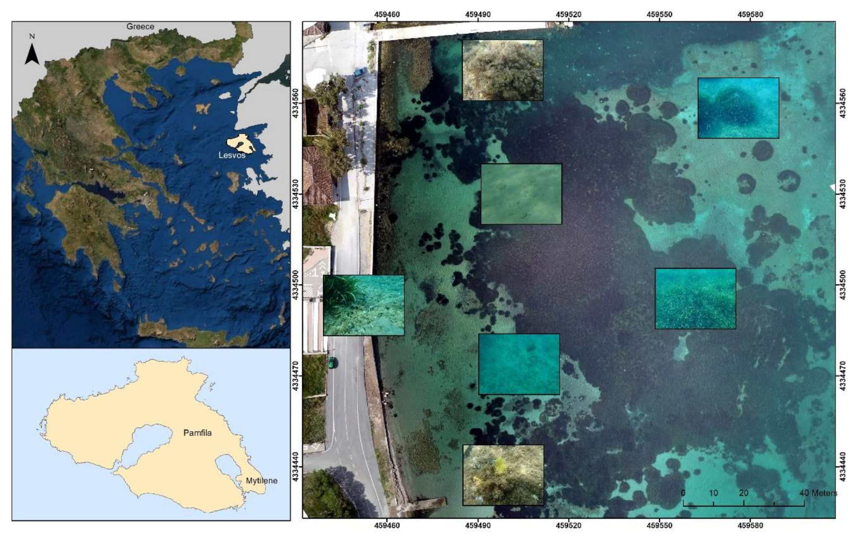
2.1. Study Area

The study area is located at Pamfila beach, which is seven kilometers north of the town of Mytilene, Lesvos Island, Greece (Figure 1). The area was chosen as its seabed has a variety of habitats and depths which are ideal for an accuracy assessment study. Moreover, the area is easily accessible and is not a restricted UAS fly region. The surveyed area is close to a small harbor situated between the shore and a small island. This area has been investigated in the past using a boat sonar system and UAS imagery for benthic mapping, as its seabed is covered by an extended seagrass meadow of Posidonia oceanica. Posidonia oceanica is one of the most important seagrass species, found only in the Mediterranean Sea, in depths extending from the surface to 40–45 m depth [16]. Seagrass meadows have a critical role in marine ecosystems, providing many services, such as favorable breeding and nursery grounds in coastal waters, sediment retention, coastal protection, improvement of water quality, and nutrient cycling [33,34].

2.2. UAS Data Acquisition Protocol

The UAS data acquisition protocol developed by Doukari et al. (2019) [25] summarizes the parameters that affect the reliability of the data acquisition process over the marine environment using UAS. The proposed UAS protocol consists of three main sections: (i) morphology of the study area, (ii) environmental conditions, and (iii) survey planning.

The first section includes parameters such as the location of the study area, the prevailing environmental conditions and phenomena prevailing in the area, and marine information (e.g., bathymetry, marine habitats). The parameters of this section are helpful for flight planning decisions, related to flight altitude, the necessary equipment for data collection, and the proper number of UAS surveys needed to capture the extent of the area. The second section is divided into weather conditions (i.e., wind speed, air temperature, sunglint) and oceanographic parameters (e.g., turbidity, tides, and phenology). These parameters affect the quality of the UAS data the most, as they produce visible artifacts on the sea-surface and the water column, affecting seabed visibility. The third section refers to the flight parameters like the UAS parameterization, the choice of the proper sensor, and flight planning. The survey planning is a demanding process as it is crucial for an efficient UAS survey [25].

In this study, the environmental parameters (i.e., wind speed, air temperature, cloud cover, wave height, sunglint) of the UAS data acquisition protocol were further examined as to their effect on the quality of UAS high-resolution orthophoto-maps. The different environmental conditions and acquisition times are investigated to assist with identifying the optimal UAS flight times and conditions. The results can lead to efficient UAS surveys in the marine environment.

2.3. UAS Data Acquisition

The UAS flights were conducted using a DJI Phantom 4 Pro system at a flight height of 70 m from the ground. The images were acquired with a nadir viewing angle (90°) and their overlap was set at 80%. The UAS flights were performed at different times and different environmental conditions. The flight plans were created through Pix4Dcapture in a grid mission with the flight lines set vertically to the shoreline. The flight settings were identical for each flight to exclude the flight parameters that may affect the quality of the orthophoto-maps. Τhis allows for the comparison of the results exclusively as to the effect of the different environmental conditions. The general weather conditions in the area were recorded from a local weather station before each UAS flight to examine their effect on the acquired imagery. We also used a handheld anemometer before each flight to verify that the wind speed is within the forecast values and sky images to evaluate the cloud coverage.

Several flights were conducted on four dates, 06/05/20, 10/05/20, 12/05/20, and 21/06/20 at different times of the day. The time variation was necessary to investigate the presence of the sunglint effect in different solar angles and how the refraction of light affects the apparent position and the shapes of the underwater objects. Additionally, underwater images and depth measurements were acquired by a scuba diver.

On the first date (06/05/20), the environmental conditions were not ideal due to the strong wind speeds ranging from 4 m/s to 6 m/s with a rough sea-state. The temperature was about 20 °C and the sky was partly cloudy. On 10/05/20, the conditions were good with small temporal differences, the wind speed ranged between 1 m/s and 2 m/s, the sea-state was calm with small wrinkles at times, the air temperature was between 18 °C and 23 °C, and the sky was clear. On 12/05/20, the wind speed measured from 3 m/s to 5 m/s, the sea swells were moderate, the temperature was 26 °C, and the sky was partly cloudy. On 21/06/20, the wind speed was 3–4 m/s, the sea-state moderate, the temperature from 25 to 27 °C, and the sky was cloudy (

Table 1. Flight conditions during the UAS surveys.

Date	6/5/2020	10/5/2020	10/5/2020	10/5/2020	12/5/2020	21/6/2020
Flight Local Time	12.00	10.00	11.00	16.00	17.00	13.00
Wind speed (m/s)	4	1	1	1	5	3
Sea-state	Moderate	Calm	Calm	Calm	Rough	Smooth
Temperature (°C)	20	19	20	23	26	27
Cloud Cover (%)	25–50%	0–25%	0–25%	0–25%	25–50%	50–75%

).

2.4. Methodology

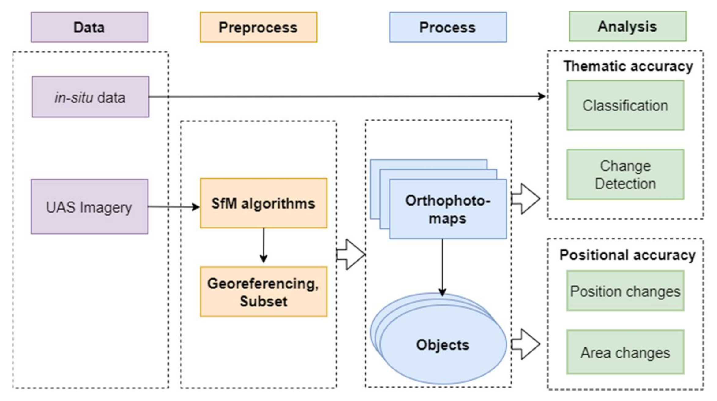
The proposed methodological workflow is divided into four parts, the data acquisition, the pre-processing of the UAS imagery, the main processing, and the analysis (Figure 2) The UAS imagery was used for the generation of high-resolution orthophoto-maps, a reference map for the geo-referencing process, and the in-situ data as training data for the classification methodology.

The UAS imagery from each acquisition was preprocessed for the generation of very high-resolution orthophoto-maps using Structure from Motion (SfM) [35] and MultiView Stereo (MVS) algorithms [36], in Agisoft Metashape [37]. The orthophoto-maps were not corrected as to their mosaicking errors as they are part of the thematic accuracy comparison. The six generated orthophoto-maps were already georeferenced by the camera positions. Their geo-reference was then corrected using a reference map to avoid shifts between them and a subset of the orthophoto-maps was selected for further analysis. The pixel size of the subsets was three centimeters, and as such, they can be used as sample data for the accuracy assessment analysis.

For selecting the reference map, we used six underwater white tiles, 40 × 40 cm in size as targets, which were placed on the sea bottom in a depth range of 0.5–4m. The white color creates strong contrasts compared to the dark coloured seagrass and can also be detected in sandy areas. The tile targets were also placed on different habitats, to increase the difficulty of observation i.e., shape of the targets. The ability to clearly distinguish the target’s shape and extent was used as an index to select a reference map. The orthophoto-map of 10/05/20 at 16.00 was selected as a reference map for parts of the accuracy assessment analysis, as its quality is highest since the underwater targets’ shape and extent can be clearly identified. In addition, the environmental conditions on that date and time were closest to the optimal values detailed in the UAS data acquisition protocol.

An example of an underwater tile, placed in a sandy area in 3.5 m depth, is shown in Figure 3. The extent of the targets was detected using an adaptive threshold with the R programming language. We used an upper and lower threshold to isolate the values corresponding to the tiles in a new raster file. The shape of the target is better displayed on 10/05/20 at 16.00, while on the dates 10/05/20 at 10.00, 11.00, and 12/05/20 at 17.00 the shape is distorted by the presence of sunglint and the wavy sea-surface. Furthermore, the target was not detected on 06/05/20 and 21/06/20 due to intense sunglint and low illumination of the seabed. The apparent extent of the targets was also calculated and compared to the actual size of the tiles, which is 0.16 m². The calculated extent of the tiles on 10/05/20 at 10.00 and 11.00 is larger than 0.16 m² (i.e., 0.19 m² and 0.20 m²), on 12/05/20 it is smaller (0.13 m²) than the actual size, and on 10/05/20 at 16.00 it is equal to 0.16 m².

The accuracy assessment of this study is divided into a thematic and positional accuracy analysis. In the thematic accuracy analysis, the reference orthophoto-map was compared to each orthophoto-map as to their quality and overall classification accuracy. Their differences were quantified and visualized using change detection methods. In the positional accuracy analysis, features of the orthophoto-maps were compared as to their differences in the centroid position, extent, and shape.

For the first part of the thematic accuracy assessment, the orthophoto maps of the different dates were classified into three classes, seagrass, sand, and mixed substrate, using the maximum likelihood (ML) supervised classification technique [38]. This technique is one of the most common supervised classifications used in remotely sensed imagery [39]. The underwater images of the habitats were matched with their orthophoto-map positions and were used as training data (Figure 1). We used twenty points of each class as sample data for the classification process. To compare the statistics of the classification classes and the overall accuracy of the classified images, we calculated the error matrices using the chosen reference classified map as a ground truth image. Furthermore, we applied the support vector machines (SVM) supervised classification technique [39], a more complex machine-learning algorithm to examine the validity of the results. SVM classification results presented similar behavior to the initial ML classification results (Appendix A,

Table A2. Support vector machines (SVM) classification statistics of the coverage percentages. On 06/05/20, parts of seagrass have been classified as sand and mixed substrate, increasing the coverage percentages of these classes. On 12/05/20, the coverage percentages are closer to the reference percentages (10/05/20, at 16.00). On 21/06/20, almost 30% of seagrass has been misclassified as sand and mixed substrate. The overall accuracies vary from 54.81 to 96.81%.

	06/05/20 12.00	10/05/20 10.00	10/05/20 11.00	10/05/20 16.00	12/05/20 17.00	21/06/20 13.00
Unclassified	0.00	0.00	0.00	0.00	0.00	0.00
seagrass	37.10	59.45	52.16	62.55	59.78	31.74
sand	41.80	29.95	32.42	29.47	32.05	47.25
mixed	21.10	10.60	15.42	7.98	8.17	21.01
OA	63.00	88.85	82.60	96.81	92.46	54.81

), and no further analysis performed using that classifier.

For the identification of the differences between the classified maps, we used a thematic change workflow. The thematic change workflow uses two classification images taken at different times and results in class transitions, from one class to another. The classified map of 10/05/20 at 16.00 was used as a reference map for the change detection comparisons for the second part of the thematic accuracy assessment. Although the change detection methods are usually used for the detection of actual changes in the marine environment, in this study they are used to emphasize the importance of the exogenous factors in the reliability of marine data.

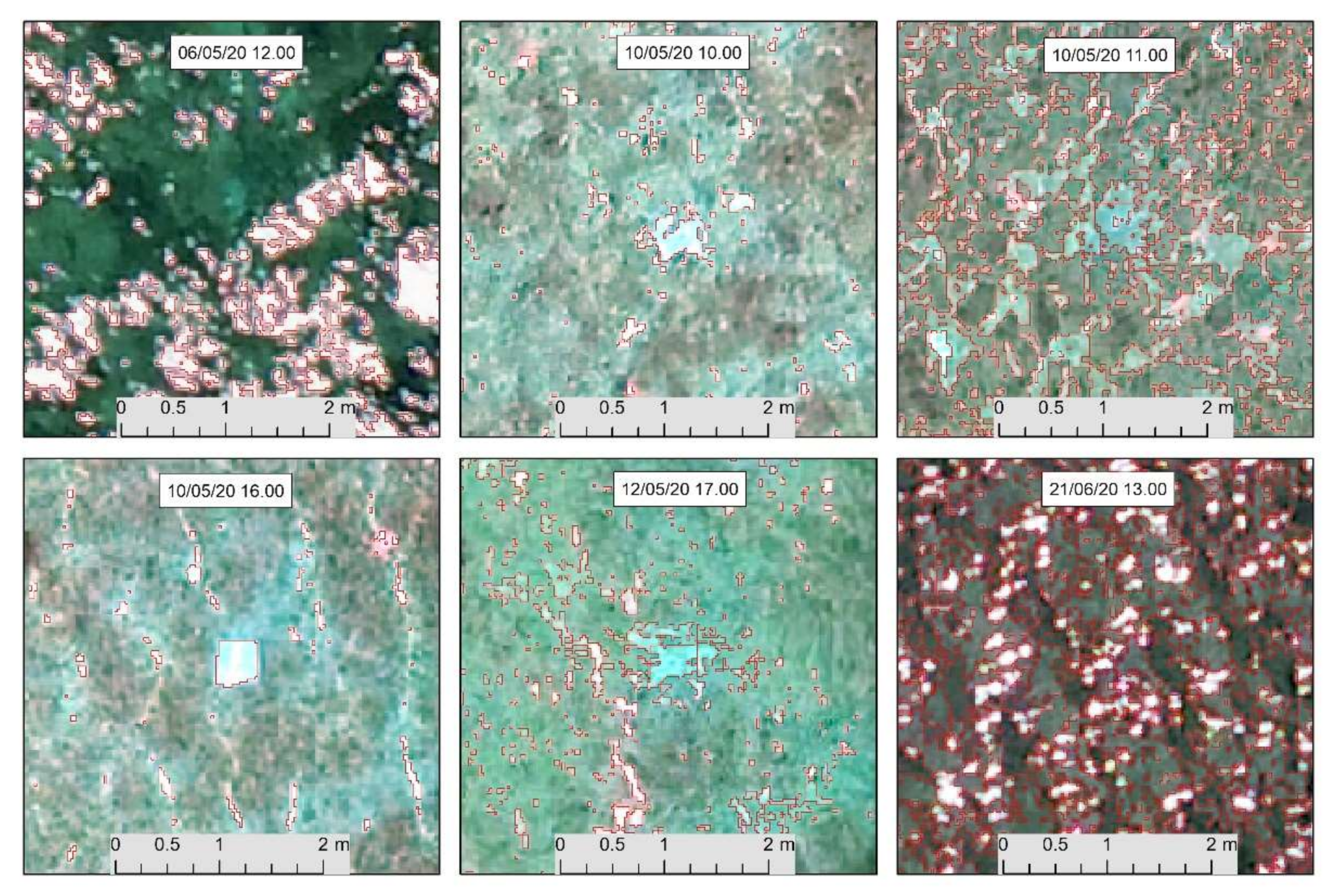
In the positional accuracy analysis, the detection and extraction of map features are necessary. After the visual inspection of the orthophoto-maps, features of seagrass patches in a unique circular shape and different sizes were chosen as comparison objects. To identify their differences in the orthophoto-maps, we analyzed their position, extent, and shape. As the orthophoto-maps were already corrected as to their position using the same reference map, we assume that possible differences in their characteristics are due to parameters that affect the sea surface and the water clarity, altering their shape.

The changes between the selected objects were extracted as polygons. Three methods were examined on polygon extraction using autonomous and semi-autonomous techniques. The first method was the use of an adaptive threshold which isolates the objects and then vectorizes them using the R programming language. An issue with this method is that the adaptive threshold does not accurately describe the extent of all objects. The second method was the segmentation of the orthophoto-map in objects which required manual merging of their parts. In the third method, we used the vectors of the classified polygons from the supervised classification method. The third method sufficiently describes the shapes of the objects, it does not require user intervention for the isolation of the shapes therefore it was preferred for the polygon extraction. Eleven objects were selected and compared as to their extents and shapes, using the objects of the reference map as sample data.

Finally, for the position comparison of the objects, we used their centroid points as they are the most reliable points to describe the position of a polygon. The centroids of the polygons were calculated by an automated process using the feature to point tool in ESRI ArcMap software, which creates point features generated from the representative locations of the input features. For polygon features, this point is located at the center of the feature. To estimate the distance errors between the calculated centroids from the reference centroids, we calculated their point to point nearest distances.

3. Results and Discussion

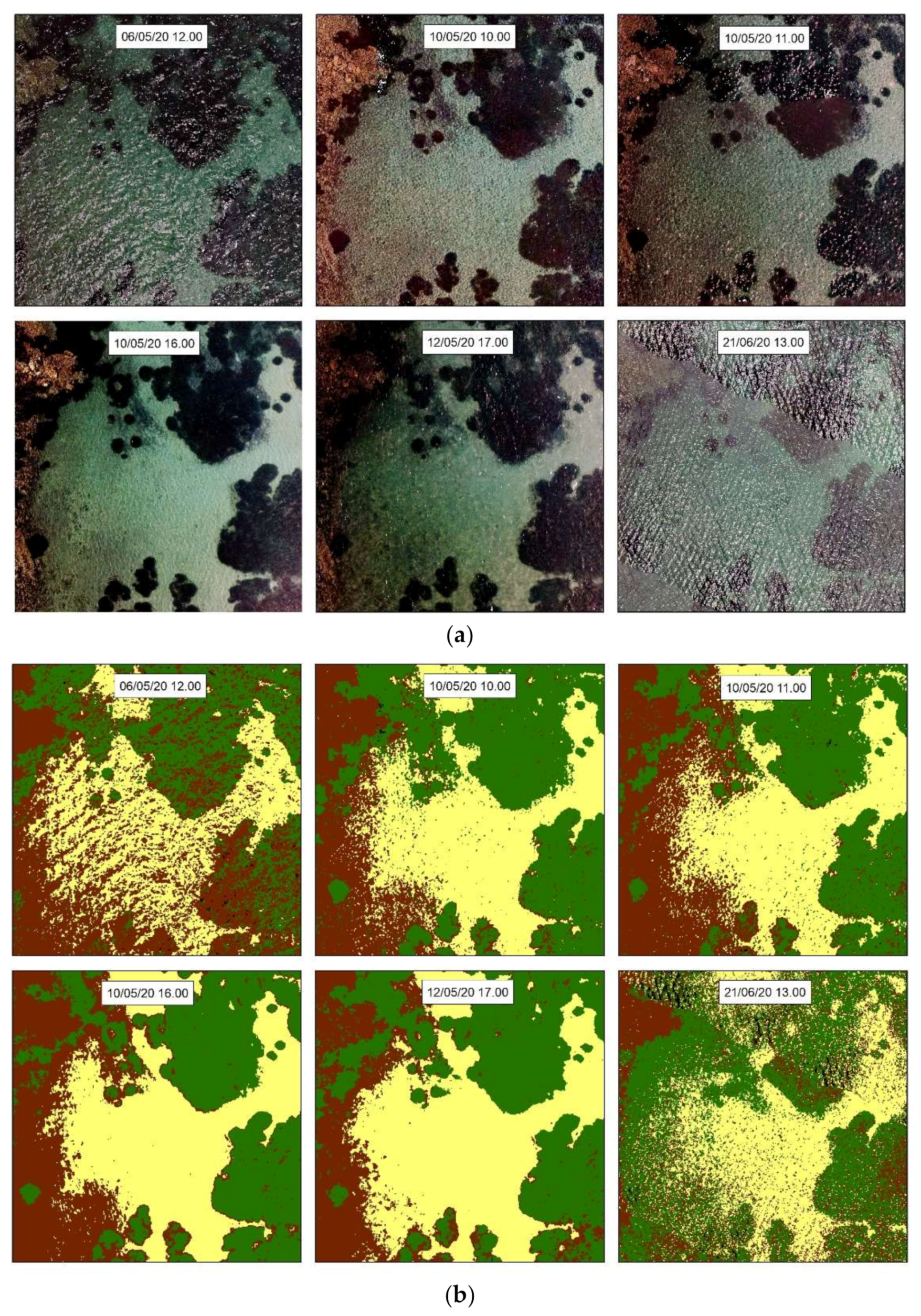
The orthophoto-maps of the different dates present obvious differences in quality, brightness, and reliability. The differences are not only due to the different acquisition times, sea-state, and environmental conditions but also to the results of the SfM process. Some of them have misaligned images and the seamlines of the mosaicking are visible, resulting in image patches in the orthophoto-maps. Subsets of the orthophoto-maps of the same study area are presented in Figure 4a.

The visual inspection of the orthophoto-maps presents several differences that can be explained by the weather conditions prevailing in the area and times of data acquisition. The orthophoto-map of 06/05/20 at 12.00 has most of its extent covered by sunglint which in combination with the wavy sea-state result in blind areas of the seabed. The conditions on 06/05/20 do not allow the distinction of the marine habitats, while parts of the orthophoto-map seem to be misaligned. The 10/05/20 orthophoto-map at 10.00 is clear enough with some wave wrinkles which alter the extent and shapes of the habitats. On the same day, at 11.00 the sea-surface was rougher, there are sunglint areas and very distinct seamlines which decrease the quality of the orthophoto-map. Later on, the same day, at 16.00 the orthophoto-map is very clear with ideal brightness which allows the habitat distinction. The conditions on that day presented temporal changes, which are attributed to the sea-state, the sunglint presence-absence, and the illumination of the seabed.

On 12/05/20 at 17.00, the orthophoto-map presents small wave wrinkles on the sea surface and sunglint areas while the brightness of the map is low. The last orthophoto-map of 21/06/20 at 13.00, presents mosaicking problems with obvious seamlines which prevent seabed visibility and habitat distinction. The extended presence of sunglint combined with the wavy sea surface led to an unsatisfactory result. The most obvious differences in the orthophoto-maps are due to sea-state conditions and sunglint presence. The visual inspection confirmed that high wind speeds and high solar elevation angles are not ideal for marine data acquisition using UAS.

The visually detected differences were quantified through the classification and change detection methods. The classification results present some differences in the capacity for the distinction of the habitats in the classified images (Figure 4b), as well as to their overall accuracies. In the classified subset of 06/05/20, the largest part of sunglint affected areas is presented as mixed substrate, instead of sand and seagrass, occupying the biggest part of the orthophoto-map. In the classified subset of 10/05/20, at 10.00, a part of the mixed substrate (top and left) is classified as seagrass, and smaller areas of sand are classified as mixed substrate probably due to waves. On 10/05/20, at 11.00, the subset presents small parts of image noise on sand and seagrass areas because of the sunglint which has been mostly classified as mixed substrate. On 10/05/20, at 17.00, the classes seem to be better districted, presenting even small parts of the mixed substrate around areas with seagrass, where there are rocks, litter, or dead leaves of seagrass.

On 12/05/20, the classified subset is similar to the previous one, with some alterations in habitat shapes. The classified subset on 21/06/20 presents some unclassified areas in black color and many misclassified areas of mixed substrate and seagrass parts. It seems that sunglint caused the most misclassified areas in the 06/05/20 image, 21/05/20 image, and parts of image noise in smaller areas in the 10/05/20 images, at 10.00 and 11.00, combined with the wavy sea-surface. The 10/05/20 image at 16.00 is of better quality, presenting the less misclassified areas and it is used as a reference map for the calculation of the confusion matrices.

The coverage percentages (%) of the classified areas are presented in

Table A1. Maximum Likelihood (ML) classification statistics of the coverage percentages, (Percentage = (Value⁄Total Value) × 100). On 06/05/20, sunglint areas and big parts of seagrass have been classified as mixed substrate, increasing greatly the coverage percentage of the class to 34.72%. In the 10/05 classified image, there are small differences in class coverages, with the biggest differences in the mixed substrate class which is increased at 11.00 due to sunglint presence. The 12/05/20 classified image has the closest coverage percentages to the reference data, with small differences due to the non-distinction of seagrass parts with the mixed substrate. On 21/06/20 the percentages show that almost 20% of seagrass has been classified as sand and mixed substrate. The overall accuracies vary from 67.92 to 97.92%.

	06/05/20 12.00	10/05/20 10.00	10/05/20 11.00	10/05/20 16.00	12/05/20 17.00	21/06/20 13.00
Unclassified	0.14	0.02	0.03	0.03	0.07	0.18
seagrass	27.71	60.73	52.29	60.10	61.43	33.68
sand	23.05	28.14	33.97	28.98	29.36	42.04
mixed	49.10	11.12	13.71	10.89	9.15	24.10
OA	67.92	93.16	89.74	97.92	95.25	70.35

(Appendix A). On both dates (06/05/20, 21/06/20), with extended sunglint presence, the seagrass class is underestimated by up to 30%, while the mixed substrate is increased to 38% on the first date, and both sand and mixed substrate to 13% on the second date. The overall accuracies of the classified images range from 68% to 95% and the Kappa indices from 0.6 to 0.9. The lowest accuracy of 67.92% is calculated on 06/05/20 and the highest of 95.25% on 12/05/20.

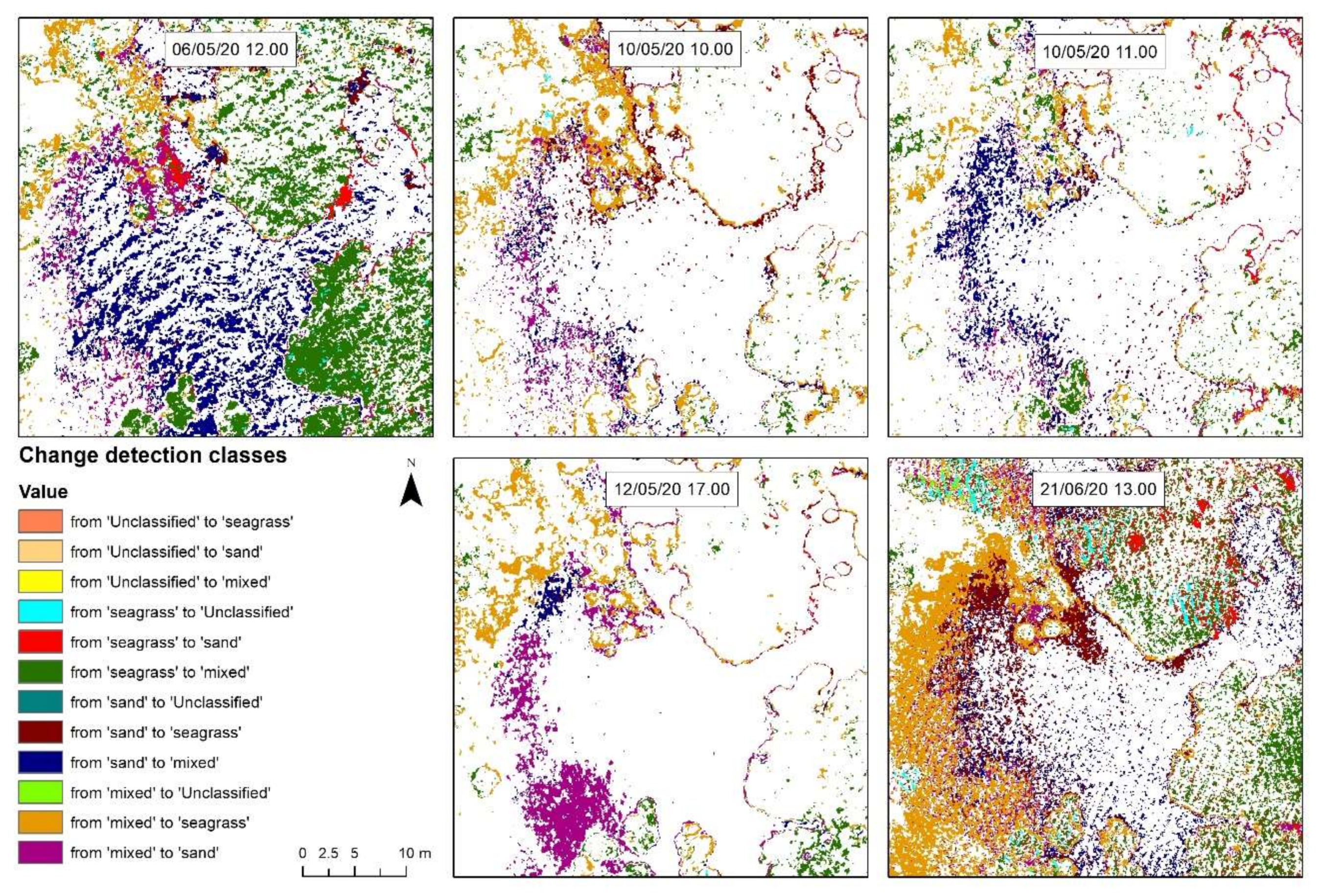
The images of the thematic change workflow show the changes between the classified images and the reference image, for each class (Figure 5). The changes represent the inaccurately classified areas due to the different environmental conditions and not actual changes in the area. It is observed that the change detection classes from seagrass to the mixed substrate (green) occupy a large part of the image on 06/05/20 and 21/06/20; also, areas have been altered from the seagrass to the sand class (red). Changes from mixed to seagrass (orange) are seen on all images with the biggest extent on the 21/06/20 image and 10/05/20 at 10.00. Changes from sand to mixed (blue) are evident in a big part of 06/05/20 and 10/05/20 at 11.00, and changes from mixed to sand (purple) are mostly shown on 12/05/20.

The change detection workflow also resulted in the percentages of changes for each class (

Table A3. Percentage changes from class to class calculated by the change detection workflow.

CLASS from	CLASS to	06/05/20 12.00	10/05/20 10.00	10/05/20 11.00	12/05/20 17.00	21/06/20 13.00
no change	no change	54.827	90.728	85.857	93.509	58.595
Unclassified	seagrass	0.002	0.002	0.002	0.003	0.001
Unclassified	sand	0.004	0.014	0.015	0.013	0.015
Unclassified	mixed	0.012	0.001	0.001	0.000	0.002
seagrass	Unclassified	0.114	0.006	0.020	0.007	0.140
seagrass	sand	1.563	1.432	6.051	0.407	15.232
seagrass	mixed	32.789	1.789	3.585	0.831	16.322
sand	Unclassified	0.002	0.00001	0.000	0.046	0.001
sand	seagrass	1.278	2.116	0.826	1.360	1.915
sand	mixed	7.423	1.149	1.424	0.620	2.263
mixed	Unclassified	0.005	0.002	0.002	0.001	0.026
mixed	seagrass	0.776	1.806	1.112	1.209	3.530
mixed	sand	1.206	0.953	1.106	1.994	1.959

, Appendix A). The largest changes have been calculated on 06/05/20, in a total of 45% of the image, 33% has been changed from seagrass to mixed substrate, 7.42% from sand to mixed, and 1.56% from seagrass to sand. Significant changes were also present on 21/06/20, in a total of 41% of the image. 16% of seagrass has been classified as sand and 15.23% as mixed substrate, 3.5% from the mixed substrate to seagrass. On both dates, the sea-surface was rough due to high wind speeds, and the presence of sunglint could not be prevented as at the time of data acquisition (12.00 and 13.00) the sun was high in the sky. The smallest changes have been calculated on 12/06/20, in a total percentage of 6.5% of the image. The conditions and the acquisition time on that day seem to be close to optimal, as the sea surface is calm, and the position of the sun prevents the presence of sunglint on the sea-surface.

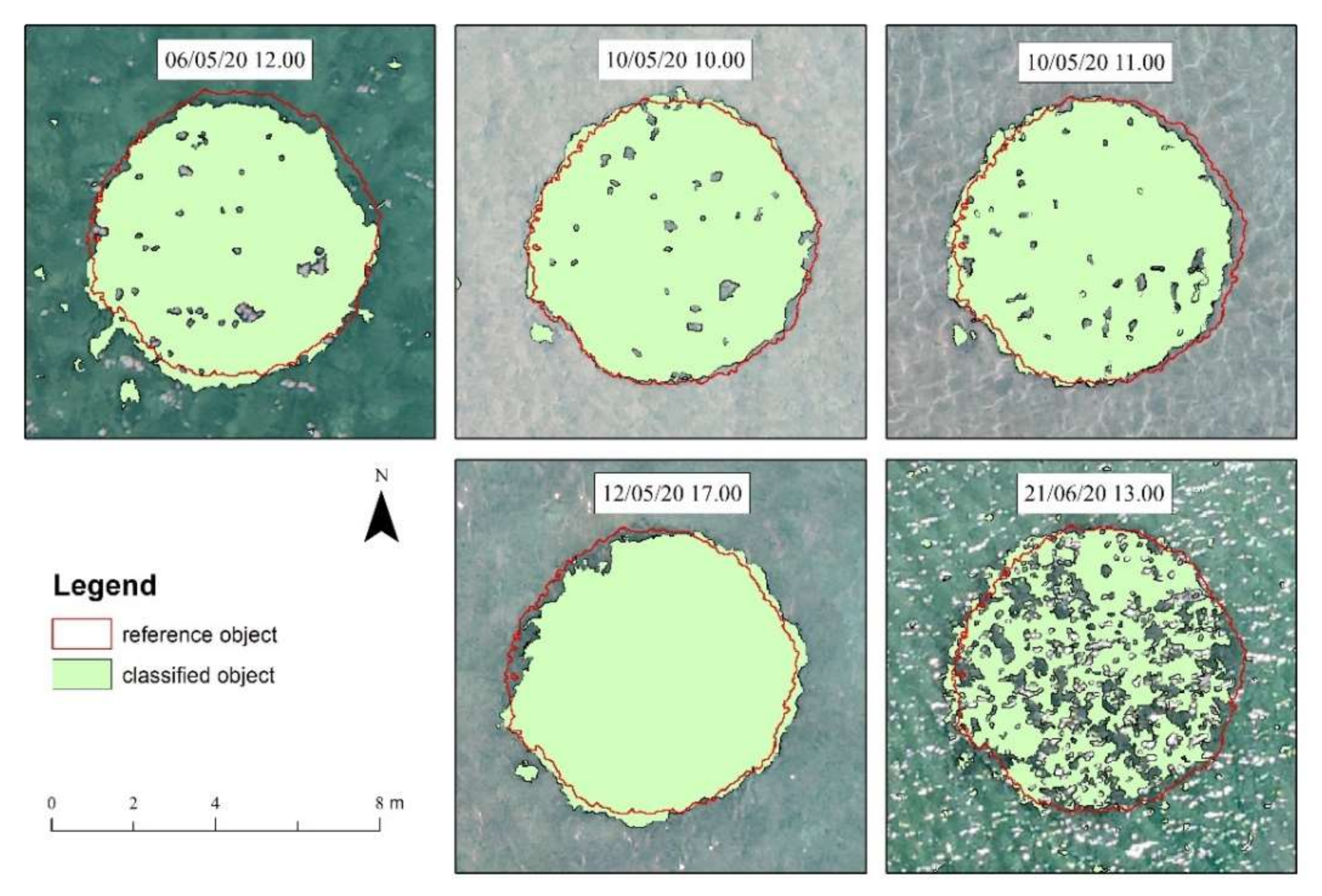
The object comparison results have many differentiations as to the areas, shapes, and positions of the objects (

Table A4. Percentage differences of object areas. The positive percentages represent the object areas that are smaller than the reference objects and the negative percentages, the object areas that are bigger than the reference objects. It is observed that eight of the objects have the biggest differences on 06/05/20 and three on 21/06/20. The lowest area differences of seven objects were calculated on 10/05/20 at 10.00, two on 12/05/20, and one on the other dates.

	6/5/2020	10/5/2020	10/5/2020	12/5/2020	21/6/2020
Objects	12.00	10.00	11.00	17.00	13.00
1	0.32	0.04	0.10	−0.21	−0.07
2	1.04	−0.65	−0.60	−0.35	−0.65
3	−1.22	−0.85	−0.16	0.25	2.34
4	0.20	−0.44	−0.03	0.14	0.53
5	1.58	0.77	1.80	−0.59	6.94
6	0.50	−0.08	0.33	0.002	−0.44
7	0.63	−0.49	−0.15	−0.43	−0.35
8	0.60	−0.07	0.22	0.11	−0.71
9	0.80	0.065	0.25	0.15	−0.70
10	0.31	−1.25	−0.14	−0.09	−0.61
11	1.06	0.02	0.32	0.26	−0.61

, Appendix A). On 06/05/20, most of the objects are smaller than the reference data, while the shapes of the objects seem to be distorted. This is mostly due to the poor quality of the orthophoto-map that does not allow the correct outline of the objects, and the extended presence of sunglint that creates gaps on the objects. On 10/05/20, the shapes and sizes of polygons are close to the reference objects, and their differences are due to the small sea swell that distorts the shape and area of the objects. On 12/05/20, the wavy sea-state and the limited sunglint areas have quite altered the shape of the objects. On 21/06/20, most of the object shapes are distorted because of the waves and the sunglint areas.

Figure 6 presents the shape and extent of object 5 on the different dates. The red polygon shows the extent and shape of the reference object. On 12/05/20 the area of the object has an increase of 1.61% which is the smallest area difference compared to the reference object and on 21/06/20 there is a 23% decrease in the area which is the highest area difference. It seems that a large part of the object has not been classified as seagrass because of the sunglint and the waves on the sea surface.

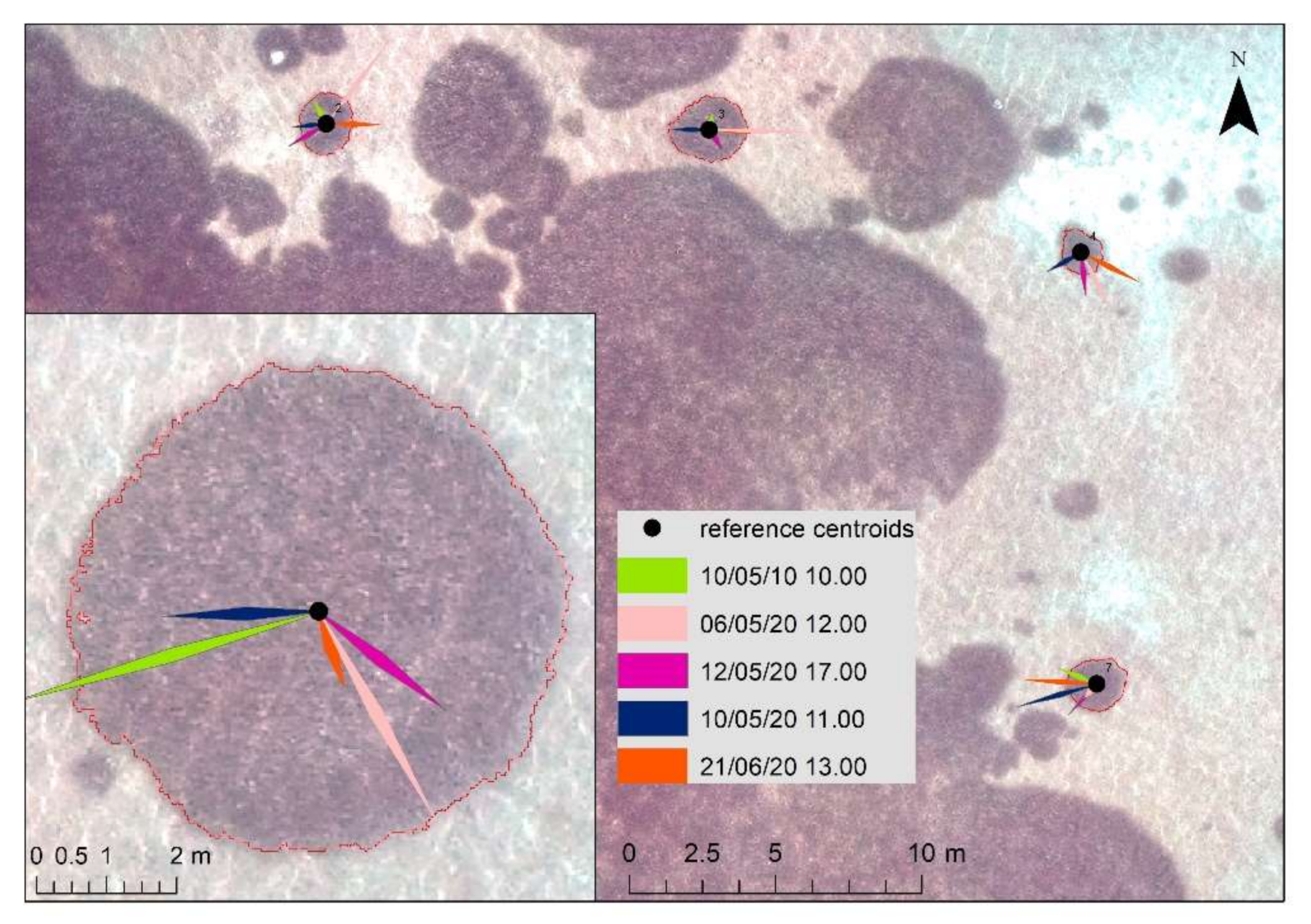
The comparison of the calculated centroids with the reference centroids on 10/05/20 at 16.00, resulted in the centroid position errors of the objects (

Table A5. Calculated centroid distance errors (m). The largest and smallest distance errors of six polygons have been calculated on 06/05/20, five on 10/05/20 at 10.00, four on 10/05/20 at 11.00, two on 12/05/20, and five on 21/06/20.

	6/5/2020	10/5/2020	10/5/2020	12/5/2020	21/6/2020
Centroids	12.00	10.00	11.00	17.00	13.00
1	0.06	0.07	0.12	0.11	0.09
2	0.39	0.10	0.13	0.16	0.20
3	0.36	0.06	0.14	0.09	0.21
4	0.25	0.02	0.15	0.16	0.25
5	0.36	0.48	0.24	0.24	0.08
6	0.05	0.04	0.04	0.08	0.11
7	0.08	0.16	0.30	0.19	0.29
8	0.13	0.08	0.05	0.05	0.25
9	0.34	0.07	0.10	0.14	0.23
10	0.13	0.20	0.23	0.10	0.06
11	0.39	0.11	0.12	0.08	0.15

, Appendix A). Considering the results in Table A5 (Appendix A), most distance errors have been calculated on 06/05/20, where the objects were distorted. An example of the positions of the calculated centroids of two objects with different sizes is presented in Figure 7. According to the calculations on the first object, the largest distance has been calculated for the centroid on 10/05/20 at 10.00, which is 0.48 m, and the least distance of 0.08 m on 21/06/20. On the second object, the largest calculated centroid distance is 0.39 m on 06/05/20, and the smallest is 0.10 m on 10/05/20 at 10.00.

It is observed that the highest errors in areas and positions are calculated on the dates that the quality of the orthophoto-maps has been affected by the environmental conditions (e.g., wind speed, waves, solar position). The differences in extent and position of the objects are most likely caused due to the refraction angle of the light which depends on the solar angle, and the environmental conditions that affect the visibility of the seabed and the habitat distinction. Although the change detection methods are usually used for the detection of actual changes in the marine environment, in this study, it was used to emphasize the importance of the exogenous factors in the reliability of the data.

The challenges and limitations of UAS data acquisition in the marine environment have been discussed in the published literature. Considering the published studies, we examined the effect of environmental conditions on the quality of UAS derived data. The use of the same flight parameters in a coastal study area, in different acquisition times and a variety of environmental conditions, allowed us to compare the generated orthophoto-maps as to their positional and thematic accuracy. Similar studies have examined the effect of environmental conditions in different coastal areas [10] and locations [22]. The reliability of the UAS acquired data through the overall accuracies of the classification have been examined as to the UAS altitude [40], and the spatial resolution [41]. In this study, we used the same UAS altitude and spatial resolution to emphasize and measure the effect of the environmental conditions on the quality of the acquired data.

Accurate habitat mapping is essential to monitor habitat changes, e.g., the decline of seagrass beds [33]. High classification errors that vary in an unpredictable way depending on sampling time and environmental conditions compromise such monitoring efforts, as they would lead to time series of habitat maps with high noise, which would mask actual changes and impede their early detection.

4. Conclusions

In this study, we examined the effect of environmental conditions on the quality and reliability of UAS remotely sensed marine information. The accuracy assessment methods confirmed that the quality of the high-resolution produced orthophoto-maps and the accuracy of the coastal habitat classification are affected by the environmental conditions prevailing in the area, and the data acquisition time. The most obvious differences in the orthophoto-maps refer to sea-state conditions and sunglint presence, while small illumination differences in the seabed have also been noticed. Visual inspection confirmed that high wind speeds and high solar elevation angles are not ideal for coastal data acquisition using UAS.

The application of the two different classifiers indicated that for the calculation of the coverage percentages in this study, it is not necessary the use of the more complex machine-learning SVM algorithm, as its results are similar to the results of the ML classifier. The analysis results confirmed that the prevalent environmental conditions during UAS data acquisition significantly affect the classification accuracies. The thematic accuracy assessment resulted in misclassified images, with a significant increase/decrease of classes on the dates that the wind speed was higher than 3 m/s and the sea surface was wavy with sunglint presence. Moreover, it has been confirmed that on data acquisition times from 11.00 to 15.00, it is almost impossible to avoid the presence of sunlight on the sea surface. Cloud cover is also an important parameter that affects the illumination of the seabed in a percentage over 25%, while cloud shadows can prevent the accurate distinction of marine habitats, increasing the probability of unreliable classification results.

The positional accuracy analysis showed important changes in the extent, shape, and position of the selected objects. Given that the objects have not changed in such a short time, we conclude that the calculated differences are attributed to changes resulting from different environmental conditions, acquisition times, and light refraction. The results of the positional accuracy analysis emphasize the importance of reliable high-resolution data for the detection of small features and the distinction of different species in coastal applications. Additionally, the accuracy assessment analysis indicates that the quality of the UAS data is affected by a plethora of factors that interact with and influence each other, thus must be considered for a sufficient UAS survey in coastal areas. These factors, i.e., wind speed, sea-surface conditions, and sunglint, reduce the available timeframes for marine data acquisition; therefore, it is important to be able to identify and understand their effect on the acquired data.

UAS is a promising tool for high-resolution mapping and for monitoring shallow habitats but caution is needed to secure optimal conditions and thus avoid serious classification errors. By adapting a proper data acquisition protocol setting optimal values for all environmental variables affecting the quality of UAS-generated orthophoto maps, the potential of UAS for habitat mapping and monitoring can be fully exploited. In this study, we validated that the acquisition time (dependent on the solar position), affects the seabed illumination and the presence/absence of sunglint on the sea surface, by presenting data acquired at different times of the day. We also proved that UAS data acquisition during non-optimal conditions could lead to imprecise and unreliable orthophoto-maps and inaccurate results of marine habitat mapping.