Article

A Tourist Attraction Recommendation Model Fusing Spatial, Temporal, and Visual Embeddings for Flickr-Geotagged Photos

1
Nansha Branch, Guangzhou Urban Planning and Design Survey Research Institute, Guangzhou 510060, China
2
Geographic Information Center, Guangzhou Urban Planning and Design Survey Research Institute, Guangzhou 510060, China
3
School of Resource and Environmental Sciences, Wuhan University, Wuhan 430079, China
4
Key Laboratory of Geographic Information Systems, Ministry of Education, Wuhan University, Wuhan 430079, China
5
Key Laboratory of Digital Mapping and Land Information Application Engineering, National Administration of Surveying, Mapping and Geoinformation, Wuhan University, Wuhan 430079, China
6
Collaborative Innovation Center of Geospatial Technology, Wuhan University, Wuhan 430079, China
*
Author to whom correspondence should be addressed.
ISPRS Int. J. Geo-Inf. 2021, 10(1), 20; https://0-doi-org.brum.beds.ac.uk/10.3390/ijgi10010020
Submission received: 13 November 2020 / Revised: 16 December 2020 / Accepted: 2 January 2021 / Published: 8 January 2021
(This article belongs to the Special Issue Geovisualization and Social Media)

Abstract

:
The rapid development of social media data, including geotagged photos, has benefited the research of tourism geography; additionally, tourists’ increasing demand for personalized travel has encouraged more researchers to pay attention to tourism recommendation models. However, few studies have comprehensively considered the content and contextual information that may influence the recommendation accuracy, especially tourist attractions’ visual content due to redundant and noisy geotagged photos; therefore, we propose a tourist attraction recommendation model for Flickr-geotagged photos which fuses spatial, temporal, and visual embeddings (STVE). After spatial clustering and extracting visual embeddings of tourist attractions’ representative images, the spatial and temporal embeddings are modeled with the Word2Vec negative sampling strategy, and the visual embeddings are fused with Matrix Factorization and Bayesian Personalized Ranking. The combination of these two parts comprises our proposed STVE model. The experimental results demonstrate that our STVE model outperforms other baseline models. We also analyzed the parameter sensitivity and component performance to prove the performance superiority of our model.

1. Introduction

With the advent of the “Web 3.0” era [1,2], the Internet users’ role has transformed from mere information receivers to producers and interactors of information. A large amount of data containing geographical location has been spontaneously generated by users, including social media check-in data, geotagged photos, etc. These data have gradually augmented or replaced the role of geographic data collected in traditional ways in geography research, including tourism geography research. According to the World Travel & Tourism Council and the World Tourism Organization statistics, the tourism industry accounts for over ten percent of global GDP [3]. Furthermore, the trip volume increases year by year, showing that the tourism industry plays an increasingly important role in the global economy [4]. In addition to the increasing scale, the tourism mode is also gradually changing. Independent travel has become the mainstream mode [5], which created tourists’ demand for personalized and intelligent travel.
New tourism demand has also promoted the transformation of the data sources and research goals in tourism geography. Specifically, applying geotagged photos to these studies is also a reflection of acclimating to such a trend. Data of geotagged photos have the advantages of containing a large amount of tourism information and reflecting tourists’ real preferences more directly [6,7]. Besides, many studies on tourist attraction recommendation systems have emerged, which aims to meet tourists’ increasing demand for intelligent and personalized tourism and solve the problem of tourist information overload [8]. The recommendation methods are generally divided into content-based and collaborative filtering (CF) methods. The content-based method uses the attributes of the items that users prefer to recommend users similar items [9]. Such a method is robust against the cold-start problem—the cold-start problem means the recommendation system can hardly make accurate recommendations when encountering new users or items [10]. Nevertheless, it relies heavily on structured and accurate features, and the accuracy of the recommendation result is comparatively low [11]. The CF-based method collects other users’ feedback to filter or rate the recommended items [10]. It has the advantages of fast speed and high accuracy, and thus it is widely used in recommendation systems. However, it cannot handle the cold-start and data sparsity problem well. It can be concluded that both of the recommendation methods have their disadvantages, leading to problems of insufficient recommending accuracy in some scenarios. Therefore, the hybrid recommendation methods that fuse both methods’ advantages have gradually become a trend [12,13]. Besides, the machine learning field’s embedding models have gradually emerged and developed in the research of recommendation algorithms. Using such a simple and efficient method to fuse content and contextual information in tourist attraction recommendations means that they can learn from each other and improve the recommendation accuracy.
New data sources and new methods have brought new opportunities to research tourist attraction recommendation methods, but they have also brought some challenges. For instance, how to select and represent the appropriate contextual and content information is a question worth considering, especially the visual information of tourist attractions, which is a kind of information that is easily ignored and difficult to extract to a certain extent because of the existence of noisy and redundant photos in geotagged photos. Therefore, we propose a tourist attraction recommendation model fusing spatial, temporal, and visual embeddings (STVE) for geotagged photos. We leverage Flickr-geotagged photos as the dataset to validate our model. The STVE model is built after some preprocessing steps, and it mainly consists of two parts: the embeddings of temporal and spatial constraint information and the embeddings of visual information. The embeddings of temporal and spatial constraint information are obtained by the negative sampling strategy of Word2Vec; then, we use matrix factorization and Bayesian Personalized Ranking and combine the embeddings of the above representative images results to get the interaction between user and visual embeddings. The gradient ascent method is used to train and update the parameters. The comparison with several other recommendation methods demonstrates that STVE has better results in recommendation quality and ranking indicators. The experiment also analyzes how the components and main parameters of STVE influence the recommendation results. The main contributions of our study are summarized below:
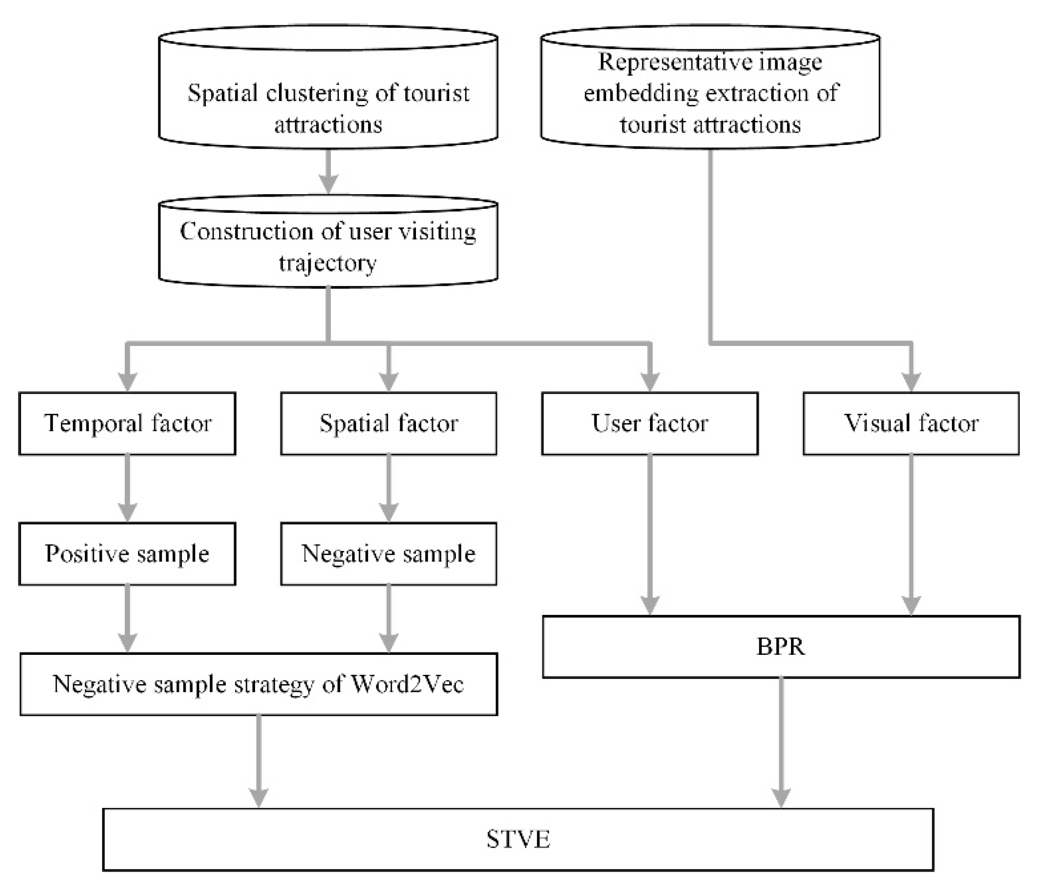
  • Given the CF-based models’ cold-start problems and the content-based models’ low accuracy problems, we propose a hybrid recommendation model for tourist attractions that fuses spatial, temporal, and visual embeddings (STVE).
  • We modify Skip-gram’s objective function to model the sequential factors in STVE, which takes advantage of Skip-gram’s characteristics that handle the sequential data well and is more in line with the actual tourist attraction recommendation scenario.
  • Given the problems that the noisy and redundant photos may exert a bad influence on the extraction of visual embeddings and the recommendation results, we propose a framework that can automatically remove the noisy and redundant photos and select representative images to extract visual embeddings of the tourist attractions for further use.
The remainder of the paper is organized as follows. Section 2 reviews the related work on tourist attraction recommendations for social media data. Section 3 introduces the preliminary and the overall framework of the study, including data acquisition, data preprocessing, and model building and training steps. Section 4 presents the performance compared with other methods, the parameter sensitivity analysis, and the component-wise study. Section 5 summarizes this paper and discusses further study.

2. Related Work

Tourist attraction recommendation can be regarded as a type of location recommendation research. Similar to recommendation methods in other fields, location recommendation methods for social media data are comprised of content- and CF-based methods. Nevertheless, with the development of recommendation system techniques, an increasing number of methods are improved by combining both methods, incorporating context and content into CF, or fusing advanced machine learning methods. Such methods can no longer be classified into content-based or CF methods and can be collectively known as hybrid methods. The selection of contextual and content information for these methods has become a nontrivial issue in location recommendation research.
Regarding contextual information in location recommendation methods, sequential information is one of the commonly considered information. It is generally modeled based on the Markov model and its variations, which calculates the probability and makes recommendations according to the transition matrix from one location to another [14,15,16]. In recent years, plenty of researchers leveraged embedding methods to model sequential information due to embedding methods. For instance, Xie et al. learned the transition from one point of interest (POI) to another with Large Information Network Embedding (LINE) [17] and generated the embedding of each POI to recommend the next POI [18]. Zhao et al. leveraged Skip-Gram to model the POI visiting trajectory [19]. Other important contextual information is the geographical distance, as one of the typical characteristics of location recommendation is that it is constrained by geographical distance. There were two major ways to model geographical distance constraints in previous studies. One is to establish a simple inverse relationship between user’s preference and geographical distance among locations, for instance, the power-law function [20,21], the Gaussian Model [22,23], and other reverse functions [24]. The other is to set a cutoff distance, and those locations whose distance from the current visiting location is larger than the cutoff distance would be filtered [15,19]. Apart from the sequential and geographical factors, other factors have also been considered in the location recommendation research, including temporal factors [25,26], the category of the locations [27], etc. The studies above considered one or two factors in their recommendation models, but few have fully integrated various factors that may affect the recommendation accuracy, not to mention the combination of content information.
The content information includes user characteristics [28,29,30], tags [31,32], and visual information. Visual information is relatively less considered because of the difficulty of extracting accurate visual information and noisy visual content in user-generated photos. Some researchers leveraged Scale-Invariant Feature Transform (SIFT) or color histograms to extract visual information [33,34], but these hand-crafted features limit the accuracy of visual information extraction to a great extent. The rise of the Convolutional neural network greatly improves visual information representation and has been applied in recommendation methods with visual content [21,35]. However, the imbalance of the number of photos in each tourist attraction and the noise and redundancy in photos still affect visual information’s representativeness. The recommendation accuracy of solely using recommendation methods based on visual content is relatively low, and the combination with other contextual information is still needed.

3. Methodology

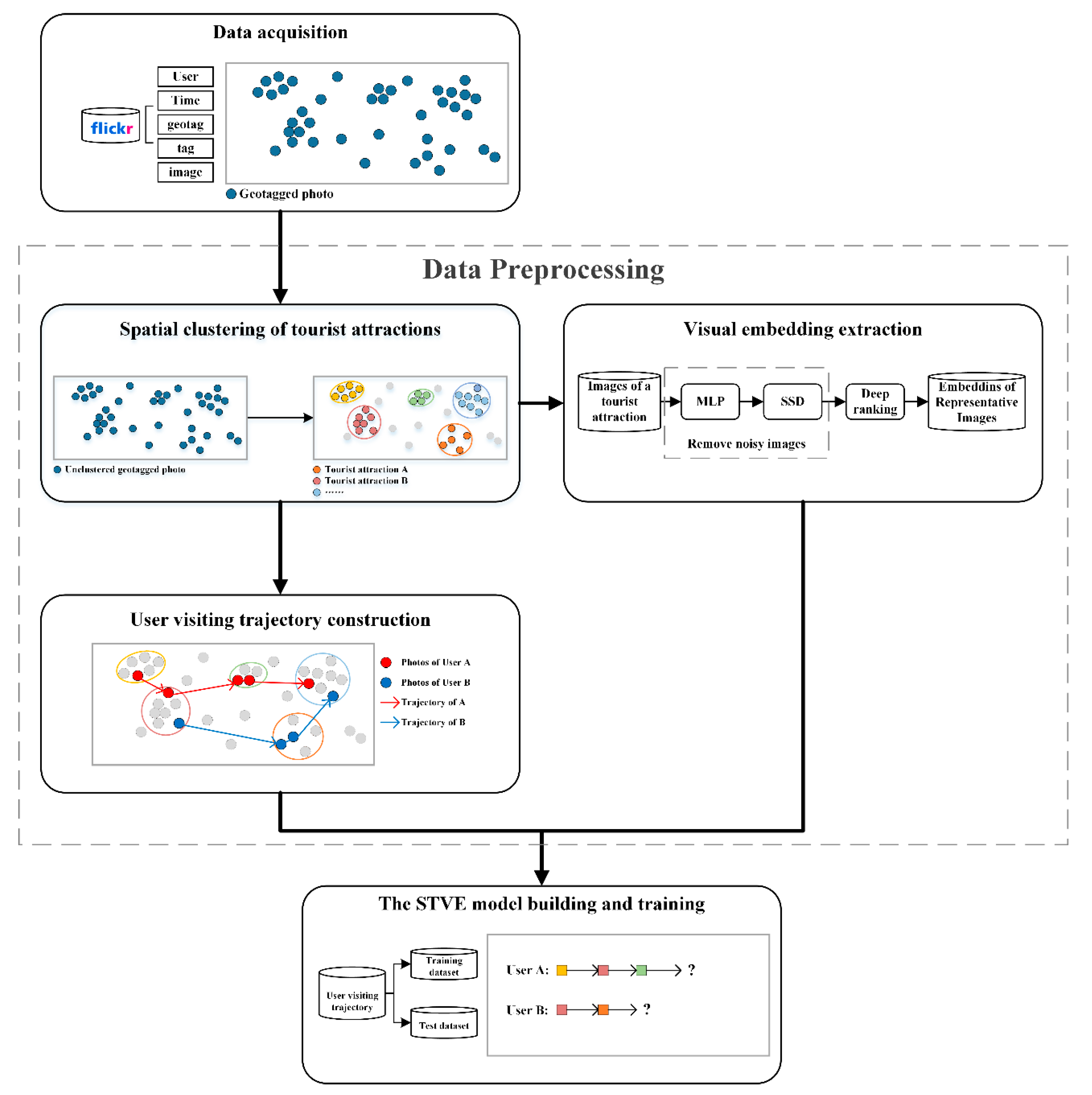
3.1. Preliminary and Framework

Before we introduce our dataset and methods, some terms need to be declared for better understanding:
Definition 1 (Geotagged photo). 
A geotagged photo is a photo with location information taken by users, represented as p . Each photo contains the identification code i d , the taken time t , the taken coordinate g , the user u , and the attached tag set X .
Definition 2 (Photo collection). 
A photo collection is all the geotagged photos in the study area within a certain time, represented as P = { p 1 , p 2 , , p | P | } .
Definition 3 (Semantic location). 
A semantic location is a location with unique semantic extracted by spatial clustering, represented as l . In our study, the extracted semantic location is a tourist attraction.
Definition 4 (Visit). 
A visit means a user’s visit to a tourist attraction within a certain time and space, represented as v = ( l , u , t , P l , u , t ) . P l , u , t represents the photo collection that the user u took when visiting the tourist attraction l at time t .
Definition 5 (User visiting trajectory). 
A user visiting trajectory is the trajectory that records all visits of the user in chronological order, represented as T u i = [ v i 1 , v i 2 , , v i | T u i | ] .
Figure 1 shows the overall framework of our study, including preprocessing steps and model building steps. Each step is illustrated in detail in the following sections.

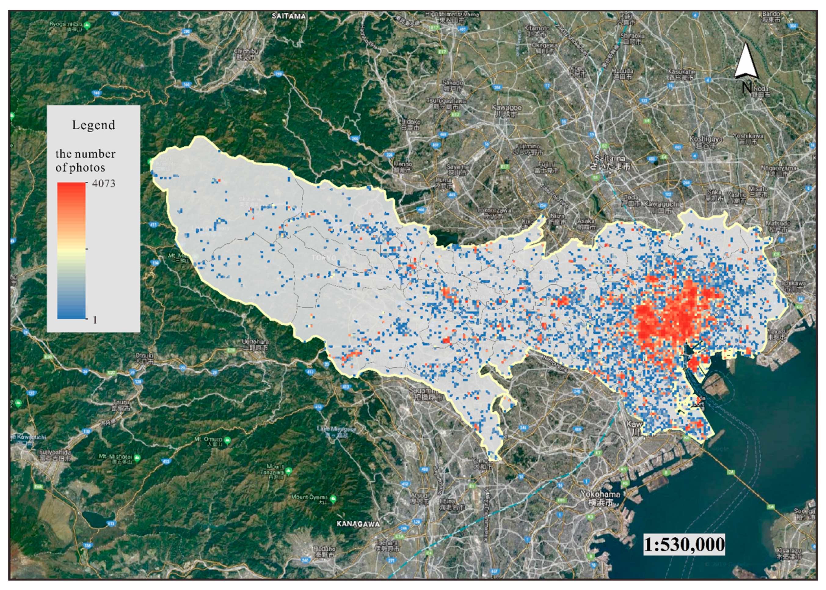
3.2. Dataset and Study Area

We leverage Yahoo Flickr Creative Commons 100 Million Dataset (YFCC100M) [36] as the experimental dataset because it can be easily downloaded from Amazon Web Services (AWS) and can provide an adequate amount of geotagged photo data. Furthermore, Menk et al. summarized that most previous studies related to tourism recommendation also used Flickr data [37], indicating its applicability in tourism research. The features of each photo we mainly use include the ID of each geotagged photo, user ID, capture time, longitude and latitude, user tags, and the images themselves.
We select the geotagged photos whose coordinates are bounded in the study area and taken within a certain time, and Tokyo is selected as the study area to evaluate our model. Tokyo is the capital city of Japan, which is also a famous tourist city. In 2018, the number of inbound tourists to Tokyo was approximately 14.24 million, and the expenditure of inbound tourists in Tokyo was about JPY 1.19 trillion [38]. Figure 2 shows the spatial distribution of Flickr photos in Tokyo. A total of 145,397 photos bounded in Tokyo and uploaded by 2750 users were used in the following experiment.

3.3. Data Preprocessing

Before the STVE model is built, some preprocessing steps are needed, including spatial clustering of tourist attractions, obtaining the visual embedding of each tourist attraction, and constructing user visiting trajectory.

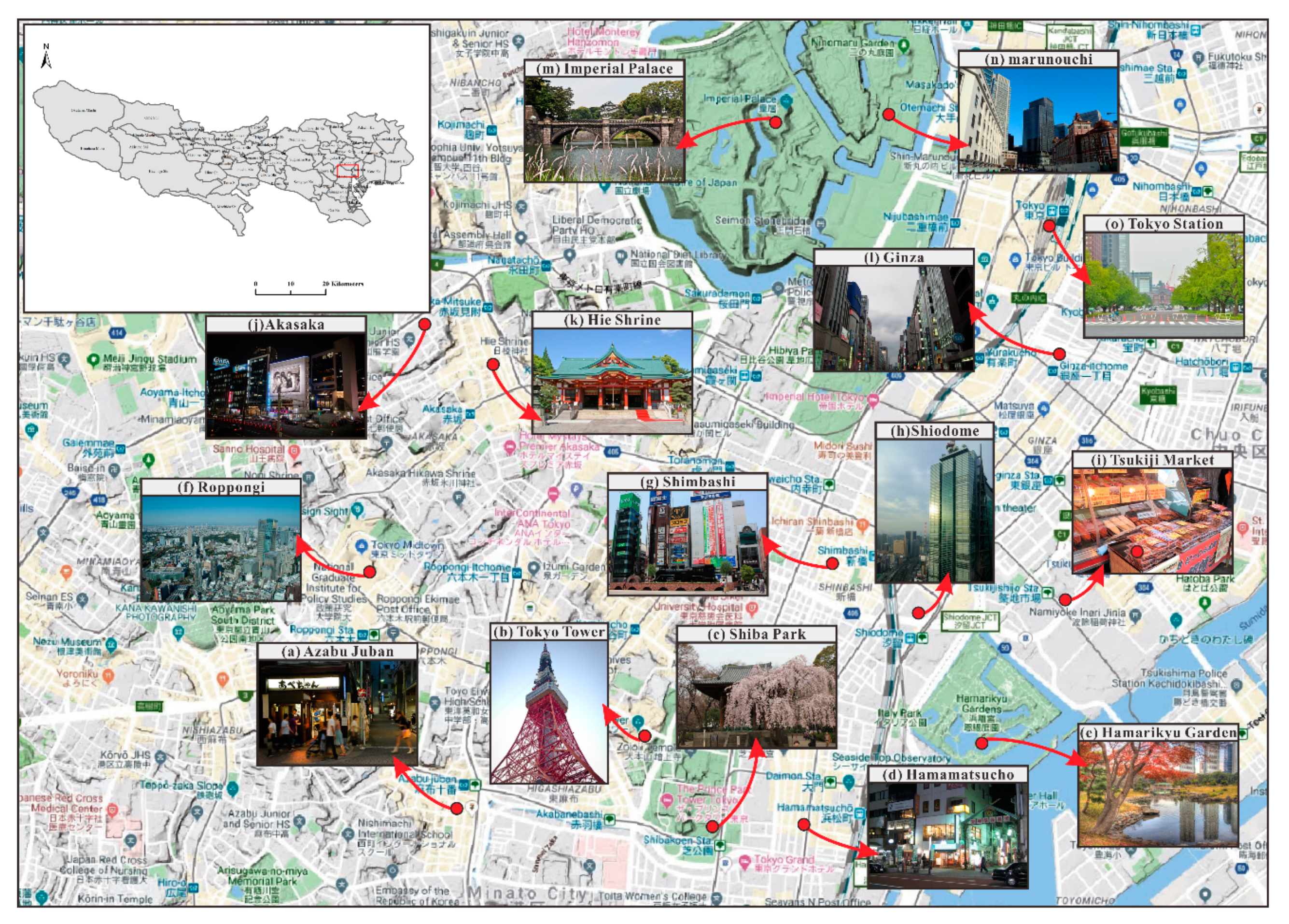
3.3.1. Spatial Clustering of Tourist Attractions

As the location information is represented as the latitude and longitude in the raw Flickr dataset, it is indispensable to cluster geotagged photos and obtain tourist attractions. We followed the clustering method in our previous study, namely the clustering method considering the spatial and semantic distance, which has proven to be effective to cluster fine-grained tourist attractions in the dense area of photos [39]. Ninety-nine tourist attractions were obtained in Tokyo after clustering, and most of them are in Chuo Ku, Minato Ku, and Chiyoda Ku. Some are shown in Figure 3, including Tokyo Tower (Figure 3b), Tsukiji Market (Figure 3i), Ginza (Figure 3l), Imperial Palace (Figure 3m), etc.

3.3.2. Visual Embedding Extraction

After clustering, we leveraged a pre-trained deep ranking model to obtain each tourist attraction’s visual embedding representation. The deep ranking model is a convolutional-based model aiming at image retrieval with fine-grained visual similarity [40]. Input each photo into the deep ranking model and will obtain a 2048-dimension embedding. It should be noted that the number of photos in each tourist attraction is not the same, and there are some photos whose visual content is unrelated to the tourist attraction (for instance, selfie). Therefore, calculating all photos’ embedding values and taking the average is not suitable to be the embedding representation of each tourist attraction. To obtain a more accurate visual representation, we made two improvements. First, we filtered two kinds of noisy photos before the photos are input into the deep ranking model: the photos whose content is mainly occupied by people are detected and removed by a single-shot multibox detector (SSD) model [41], and the photos that mainly displayed the objects are filtered by Multilayer Perceptron pre-trained by the Caltech 101 dataset [42] and the Places2 dataset [43]. Second, after obtaining the embeddings of the remaining photos from the deep ranking models, we calculate the Euclidean distance of each embedding from all other embeddings and sort them in ascending order. If the distance between the two embeddings is small, the corresponding two photos’ visual content is similar. Therefore, if an embedding’s distance among all other embeddings is small, this photo’s visual content is comparatively typical and representative. For each tourist attraction, we calculated the average of the top n embeddings with the smallest distance from other embeddings, and the result will be further used as the visual embedding of this tourist attraction, represented as e ¯ l j :
e ¯ l j = k = 1 n e l j k n
where e l j k represents the k -th embedding in the top n list of the j -th tourist attraction, and we set n as 50 in this study. The visual embedding of each tourist attraction was fused into the recommendation model.

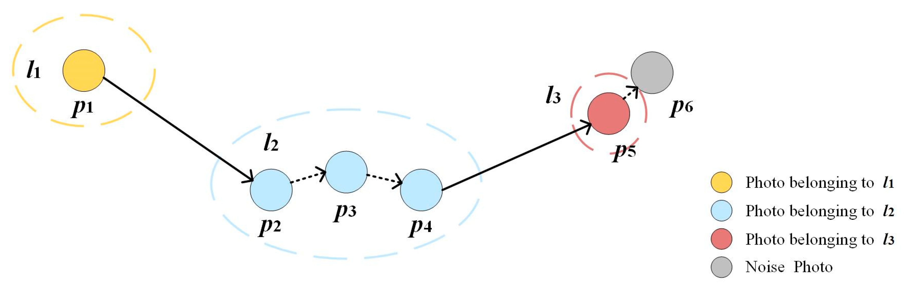
3.3.3. User Visiting Trajectory Construction

Constructing the user visiting trajectory is needed to be the training data of the STVE model. Unlike Foursquare or other social media check-in data that can connect a user’s check-in records in chronological order to be the user visiting trajectory, the user of geotagged photos may take more than one photo when visiting a tourist attraction within a short time (as shown in the three photos in l 2 in Figure 4). Another inevitable problem is that some photos cannot be clustered into any tourist attraction due to the nature of density-based clustering with noise. Therefore, we set a time threshold Δ t and a distance threshold Δ d i s to judge whether the photos taken at the adjacent time should be merged as the same visit. Sort each user’s photos in chronological order, starting from the first photos and looping through them. If the current photo and the next photo have been clustered into the same attraction and the interval of their shooting time is less than Δ t , merge them as the same visit. If at least one of the current photo and the next photo is not clustered, judge whether the shooting time interval is less than Δ t and the distance of the two photos is less than Δ d i s . If both are true, merge them as the same visit. After constructing the user visiting trajectory, we remove users who visited no more than four attractions, and the final number of trajectories (users) is 1,801. We select the former 80% of each trajectory as the training data and the remaining 20% as the final evaluation test data.

3.4. Model Description and Optimization

In the following section, we describe our STVE model, including the spatial–temporal embedding part, the visual embedding part, and model optimization. The structure of STVE and the connection between preprocessing steps are shown in Figure 5, and some important notations in the STVE model are listed in Table 1.

3.4.1. Spatial–Temporal Embedding

We first modeled the sequential characteristics of tourist visiting trajectories with Skip-gram’s principle, because Skip-gram, as a kind of Word2Vec methods, can well handle the sequential data like sentences. The objective function of Skip-gram is to maximize the probability of the contextual words given the center word, represented as:
Γ = w t | C | t k i t + k p ( w i | w t )
where C represents the whole training corpus, and w i represents the contextual word of w t within the window size k . Both w t and w i belong to the corpus C . We regard one user visiting trajectory as a sentence and each tourist attraction in trajectory as each word. With Skip-gram’s objective function, we infer the contextual tourist attractions given the center attractions in the trajectory. However, in the scenario of natural language sentences, the strategy of contextual word selection of Word2Vec is without direction, while in the tourist attraction recommendation scenario, it is more in line with the actual situation to predict the next attraction given the currently visited attraction. In this way, we modify the conditional probability as Equation (3):
= T u i T 1 | T u i | l k , l k + 1 T u i log P ( l k + 1 | l k )
where T represents the whole visiting trajectories of all users; l k and l k + 1 represent the k -th and ( k + 1 ) -th visited tourist attractions of trajectories belonging to user u i respectively, and k = 1 , 2 , , | T u i | 1 . P ( l k + 1 | l k ) represents the conditional probability from l k to l k + 1 . Similar to the target of Word2Vec sentence training, Equation (3) maximizes these conditional probabilities in the whole dataset T .
Apart from the influence of sequential characteristics, the time of the day may also influence users’ selection of visiting attractions. The heat map in Figure 6 shows the users’ visiting patterns of fifty randomly selected Tokyo attractions at different hours within one day. It can be seen that the visiting patterns for different tourist attractions are not the same. For instance, the visiting hours for the first two attractions (ID 0 and 1) in Figure 6 are concentrated between 10 a.m. and 4 p.m., while some tourist attractions (such as ID 43 and 44) are discretely distributed between 11 a.m. and 10 p.m. Therefore, the recommendation model should also be considered the influence of the time of the day.
Suppose the target recommendation scenario is to infer the most likely visiting attractions given the previous visiting attractions and the current time, the equation adding the temporal factor based on Equation (3) can be formulated as the following:
= T u i T 1 | T u i | ( l k , l k + 1 ) T u i log P ( l k + 1 | l k , t k + 1 )
where t k + 1 represents the time that user u i visited the ( k + 1 ) -th tourist attraction. We map the time of the day into integer values from 0 to 23 to avoid the problems of too many time slots and data sparsity. For instance, if a user visits a tourist attraction between 8 a.m. and 9 a.m. (not including 9 a.m.), the visiting time will be mapped to 8.
The SoftMax function is used to define the conditional probability P ( l k + 1 | l k , t k + 1 ) and train the latent factors of l k , l k + 1 and t k + 1 (denoted as v l k , v l k + 1 and v t k + 1 , respectively). Two symbols v ^ c t and v ^ n are introduced for a better description, and they are defined as follows: v ^ c t = v l k v t k + 1 , v ^ n = v l k + 1 v l k + 1 , where represents the concatenation operator. The inner product of v ^ c t and v ^ n can be denoted as follows: v ^ n v ^ c t = v l k v l k + 1 + v t k + 1 v l k + 1 . Then P ( l k + 1 | l k , t k + 1 ) can be formulated as:
P ( l k + 1 | l k , t k + 1 ) = exp ( v ^ n v ^ c t ) l k L exp ( v ^ n v ^ c t )
However, the cost of computing Equation (5) is impractically high because of the SoftMax function. Therefore, the negative sampling method is leveraged as a computationally efficient approximation algorithm in Equation (4). Therefore, Equation (4) can be transformed into Equation (6):
= T u i T 1 | T u i | l k , l k + 1 T u i ( log σ ( v ^ n v ^ c t ) + ( l k , l n e ) T u i k n e log ( 1 σ ( v ^ n e v ^ c t ) ) )
where σ ( x ) is the Sigmoid function; l n e represents the negative sample attractions, and k n e is the number of negative samples. Due to spatial distances constraint, tourists may prefer a tourist attraction closer to the current visiting tourist attraction. In other words, tourists are less likely to choose a tourist attraction far away from the current visiting one. Therefore, we introduce this idea of spatial distance constraint to the process of negative sampling, i.e., the negative samples are not randomly chosen but are chosen from those attractions whose distance with the current visiting attraction is larger than a predefined distance threshold. The set of negative samples can be formulated as Equation (7):
L n e g = { l n e g L \ l k + 1 : d i s ( l k , l n e g ) Δ d i s }
where Δ d i s is a predefined distance threshold. Substitute L n e with L n e g in Equation (6), and the final representation of spatial-temporal embedding can be represented as:
S T = T u i T 1 | T u i | l k , l k + 1 T u i ( log σ ( v ^ n v ^ c t ) + ( l k , l n e g ) T u i k n e log ( 1 σ ( v ^ n e v ^ c t ) ) )

3.4.2. Visual Embedding

As analyzed above, the visual factor is also one of the essential factors that impact tourists’ decision to choose tourist attractions. Therefore, the recommendation model should be fused with visual information. Enlightened by Visual Bayesian Personalized Ranking (VBPR) proposed by He et al. [44], we also try to fuse tourist attractions’ visual embeddings into matrix factorization and Bayesian Personalized Ranking. The matrix factorization of “users—tourist attractions” can be established as:
= v u i · v l j
where v u i is the embedding of the user i , and v l j is the embedding of the tourist attraction j . The dimension of them are both f 2 . We leverage the inner product of the visual embedding e ¯ l j generated in Section 3.3 and a parameter matrix W u l to represent v l j :
v l j = W u l · e ¯ l j
where W u l is a f 2 × f e parameter matrix, and f e is the number of dimensions for visual embedding e ¯ l j (2,048 as mentioned above). Substitute v l j with Equation (10) and further introduce the bias term β in Equation (9), the representation of visual embedding can be formulated as:
V = v u i · ( W u l · e ¯ l j ) + β · e ¯ l j
Optimize V with VBPR, which assumes that the user prefers this attraction over all other attractions. Randomly select the negative sample l n e . Suppose the number of negative samples is k n e , then V can be formulated as:
V = 1 k n e v u i · ( W u l · ( e ¯ l j e ¯ l n e ) ) + β · ( e ¯ l j e ¯ l n e )
For the whole training dataset, the users’ visual preference for the tourist attractions can be modeled as Equation (13):
V = T u i T 1 | T u i | l k T u i 1 k n e v u i · ( W u l · ( e ¯ l j e ¯ l n e ) ) + β · ( e ¯ l j e ¯ l n e )

3.4.3. Model Learning

We combine Equation (8) with Equation (13) by the linear weighted sum method, and the objective function of the proposed STVE model that fuses spatial, temporal, and visual information, which is formulated as:
θ = argmax θ ( α · S T + ( 1 α ) · V )
where θ is the parameter set that can maximize the value of ( α · S T + ( 1 α ) · V ) through training, and θ = { V L , V N , V T , V U , W u l , β } . v l k , v l k + 1 , v t k + 1 , and v u i shown in the equation of Section 3.4.1 and Section 3.4.2 belong to the embedding of the corresponding subscript in matrix V L , V N , V T , and V U , respectively. α is the linear parameter to control the weight of S T and V , and we set it as 0.7 in this experiment.
The detail of the learning process of STVE is shown in Algorithm 1. The input of STVE training includes the training dataset T and the parameter set θ . We leverage mini-batch gradient ascent to update the parameters, and we set the ratio parameter b as 0.5. The training epoch is m a x _ e p o c h , and η 1 and η 2 are the learning rate of S T and V , respectively. Δ d i s is the parameter of the cutoff distance threshold. First, initialize all the parameters with a normal distribution (Line 1), and the formula for updating parameters is as follows:
θ t + 1 = θ t + η · ( θ ) θ
where η is the learning rate. Update v t k + 1 , v l k and v l k + 1 for each user’s top ( | T u j | 1 ) visited attractions (Line 6 to 9), and select k n e negative samples from the L n e g to update v t k + 1 , v l k and v l m (Line 10 to 14), which is the updating process of the parameters in the S T part. Regarding the V part, we define x ^ u i l k l n as:
x ^ u i l k l n = x ^ u i l k x ^ u i l n = v u i · ( W u l · ( e ¯ l k e ¯ l n ) ) + β · ( e ¯ l k e ¯ l n )
where x ^ u i l k l n and x ^ u i l n are defined by Equation (11). Update v u i , β and W u l with VBPR (Line 17 to 20):
( u i , l j , l k ) T l n   σ ( x ^ u i l j l k ) λ θ | | θ | | 2
where λ θ is the regularization parameter. Here we set v u i , β and W u l as the same value λ .
Algorithm 1: the STVE model
Input: T -dataset; θ = { V L , V N , V T , V U , W u l , β } ; m a x _ e p o c h -the number of epoch; b –the ratio of batch size; η 1 -the learning rate of S T ; η 2 -the learning rate of V ; Δ d i s -cut distance; k n e -the number of negative sample in S T ; k n e -the number of negative sample in V ; λ -regularization parameter.
Output: θ
1Initialize θ with Normal Distribution
2for i = 0 ; i < m a x _ e p o c h do
3 T u s   RandomlySelect ( T u , b )
4for j = 0 ; j < | T u s | ; T u j T u s do
5  for k = 0 ; k < | T u j | ; l k T u j do
6   if k < | T u j | 1 do
7     v t k + 1 v t k + 1 + α η 1 ( 1 σ ( v ^ n v ^ c t ) ) v l k + 1
8     v l k v l k + α η 1 ( 1 σ ( v ^ n v ^ c t ) ) v l k + 1
9     v l k + 1 v l k + 1 + α η 1 ( 1 σ ( v ^ n v ^ c t ) ) ( v t k + 1 + v l k )
10     L n e g = { l n e g L \ l k + 1 : d i s ( l k , l n e ) Δ d i s }
11    for m = 0 ; m < k n e ; l m L n e g do
12      v t k + 1 v t k + 1 α η 1 ( 1 σ ( 1 v ^ n v ^ c t ) ) v l m
13      v l k v l k α η 1 ( 1 σ ( 1 v ^ n v ^ c t ) ) v l m
14      v l m v l m α η 1 ( 1 σ ( 1 v ^ n v ^ c t ) ) ( v t k + 1 + v l k )
15    end
16   end
17   for n = 0 ; n < k n e ; l n L n e do
18     v u i v u i + ( 1 α ) η 2 ( 1 σ ( x ^ u i l k l n ) ) W u l ( e ¯ l j e ¯ l k ) λ v u i
19     β β + ( 1 α ) η 2 ( 1 σ ( x ^ u i l k l n ) ) ( e ¯ l j e ¯ l k ) λ β
20     W u l W u l + ( 1 α ) η 2 ( 1 σ ( x ^ u i l k l n ) ) v u i ( e ¯ l j e ¯ l k ) T λ W u l
21   end
22  end
23end
24end

4. Experimental Result

4.1. Experiment Settings

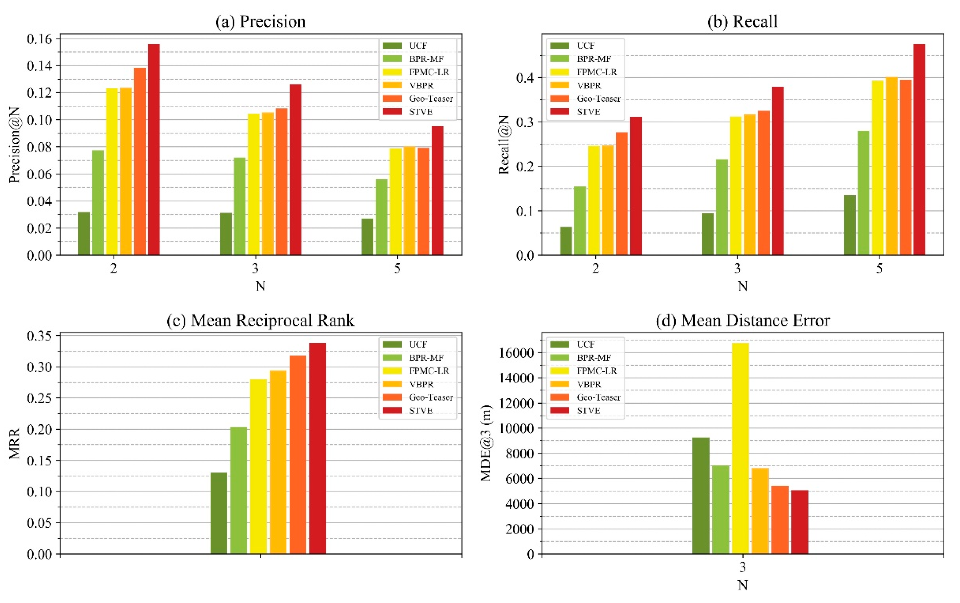
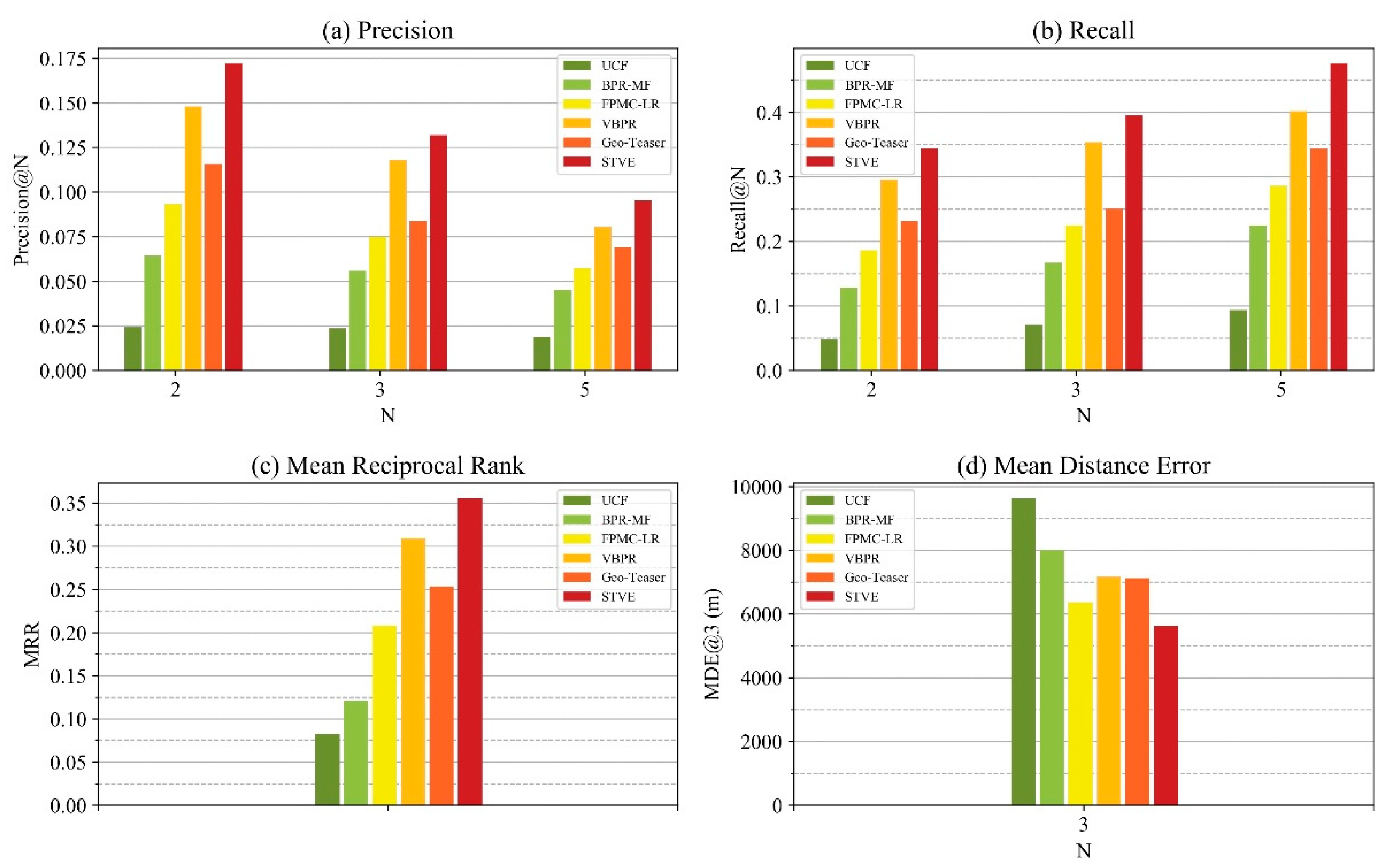
4.1.1. Evaluation Metrics

We leverage four metrics to evaluate our STVE model, including precision, recall, mean reciprocal rank (MRR), and mean distance error (MDE). Precision@N refers to the proportion of the ground-truth tourist attractions that are included in the top-N recommended list, and Recall@N means the ratio between the number of ground-truth attractions in top-N recommended results and the number of tourist attractions that the user visited; these are two common metrics to evaluate the recommendation quality and can be formulated as Equations (18) and (19), respectively:
P r e c i s i o n @ N = 1 | T | T u i T 1 | T u i | × l k T u i | R N ( u i ) l k | N
R e c a l l @ N = 1 | T | T u i T 1 | T u i | × l k T u i | R N ( u i ) l k | | l k |
where R N ( u i ) is the set of top- N recommendation results, and l k represents the actual tourist attraction that the user visited.
MRR is the recommendation ranking metrics, which is defined as:
M R R = 1 | T | T u i T 1 | T u i | × 1 l k T u i r a n k l k
where r a n k l k is the ranking number of the ground-truth attraction in the recommended list.
MDE calculates the average minimum geographical distance between the ground-truth tourist attraction and any of the top- N predicted attractions. It is not a general metric to evaluate the recommendation system, but it can be used to evaluate the distance error of the recommendation results, which was also used in the study of Yao et al. [45] related to location prediction. MDE can be formulated as:
M D E @ N = 1 | T | T u i T 1 | T u i | × l k T u i , l k n R N ( u i ) d i s ( l k , l k n )
where l k n represents any attraction in the top- N list, and d i s ( x , y ) represents the distance between x and y , defined by Haversine distance. A smaller value of MDE indicates better performance in distance error.

4.1.2. Comparison Methods

We chose several recommendation models to compare the performance of our model, including:
  • User-based Collaborative Filtering (UCF): UCF is a classic memory-based recommendation model that mainly uses other users with similar preferences to make recommendations [46,47].
  • Bayesian Personalized Ranking-Matrix Factorization (BPR-MF): BPR-MF is a simple “user-item” matrix factorization method optimized with Bayesian Personalized Ranking.
  • Factorizing Personalized Markov Chains with the localized regions (FPMC-LR): FPMC-LR [15] is a recommendation method that was improved by adding the geographical distance constraint to Factorizing Personalized Markov Chain methods (FPMC) [14].
  • VBPR: VBPR is a matrix factorization model with visual information aimed at online shopping recommendations [44].
  • Geo-Teaser: Geo-Teaser was a method that integrates temporal and geographical information with the negative sampling strategy of Word2Vec and hierarchical pairwise ranking to make recommendations [19].

4.2. Performance Comparison

Figure 7 shows the performance of the STVE model and other baseline methods in the metrics of precision (Figure 7a), recall (Figure 7b), MRR (Figure 7c), and MDE (Figure 7d). From Figure 7, we can conclude that the STVE model outperforms any other baseline methods in four metrics. It performs particularly well on recall and MRR, indicating the relatively high proportion of the recommended results hitting the ground-truth tourist attractions, and the high average ranking of the ground-truth tourist attractions in the recommended list. Additionally, the STVE model’s performance in MDE is also superior to other models; the gap between FPMC-LR and STVE is particularly large, which may be related to the different strategies of negative sample selection between them. The high MDE value of FPMC-LR demonstrates that selecting negative samples within the cutoff distance may not be in line with the actual situation, as a closer distance between the current attractions and the recommended ones seems to be more likely to attract tourists to visit them.
We further analyze the results of other baseline models. As the only memory-based CF method, the UCF’s performance is far inferior to other models in four metrics, revealing the difficulty of memory-based CF in solving the data sparsity and cold-start problem. On the other hand, even though BPR-MF, the classic model-based CF, does not fuse any contextual and content information, it still performs better than UCF, which implies that selecting the model-based CF as the basic method of the STVE model can effectively improve the recommendation accuracy and overcome the problem of data sparsity compared with the memory-based CF. FPMC-LR and VBPR are improved models that add context or content based on BPR-MF. Both obtain better results than BPR-MF, which shows that selecting and fusing appropriate context and content into matrix factorization can improve the recommending accuracy. Finally, as a model that owns the most similar model structure and factors with STVE, Geo-Teaser is superior to all other baseline models in performance. Though such results imply the advantages of the model structure of Geo-Teaser, the performance of Geo-Teaser still ranks second to STVE. It may be due to two reasons: first, when modeling the sequential information with Word2Vec, Geo-Teaser undirectedly takes the previous and the next visited attractions of the current attractions as the contextual “words”. STVE improves the conditional probability in Equation (3) as predicting next attraction given the current attraction is more in line with the actual situation; second, Geo-Teaser considers only spatial and temporal (sequential) factors, while STVE includes not only the above factors but also the visual factor, which may be another important reason that influences the recommendation accuracy.

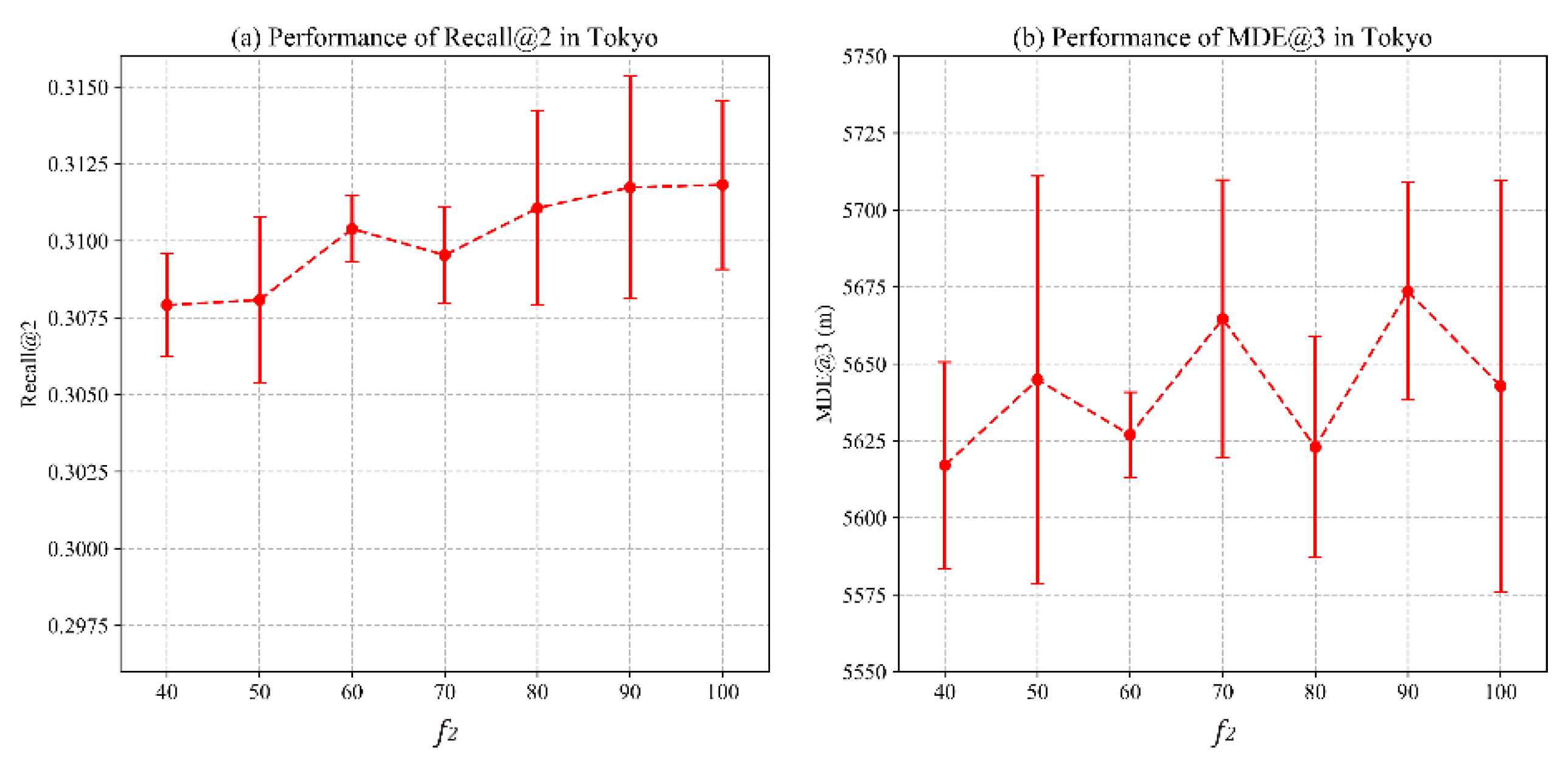
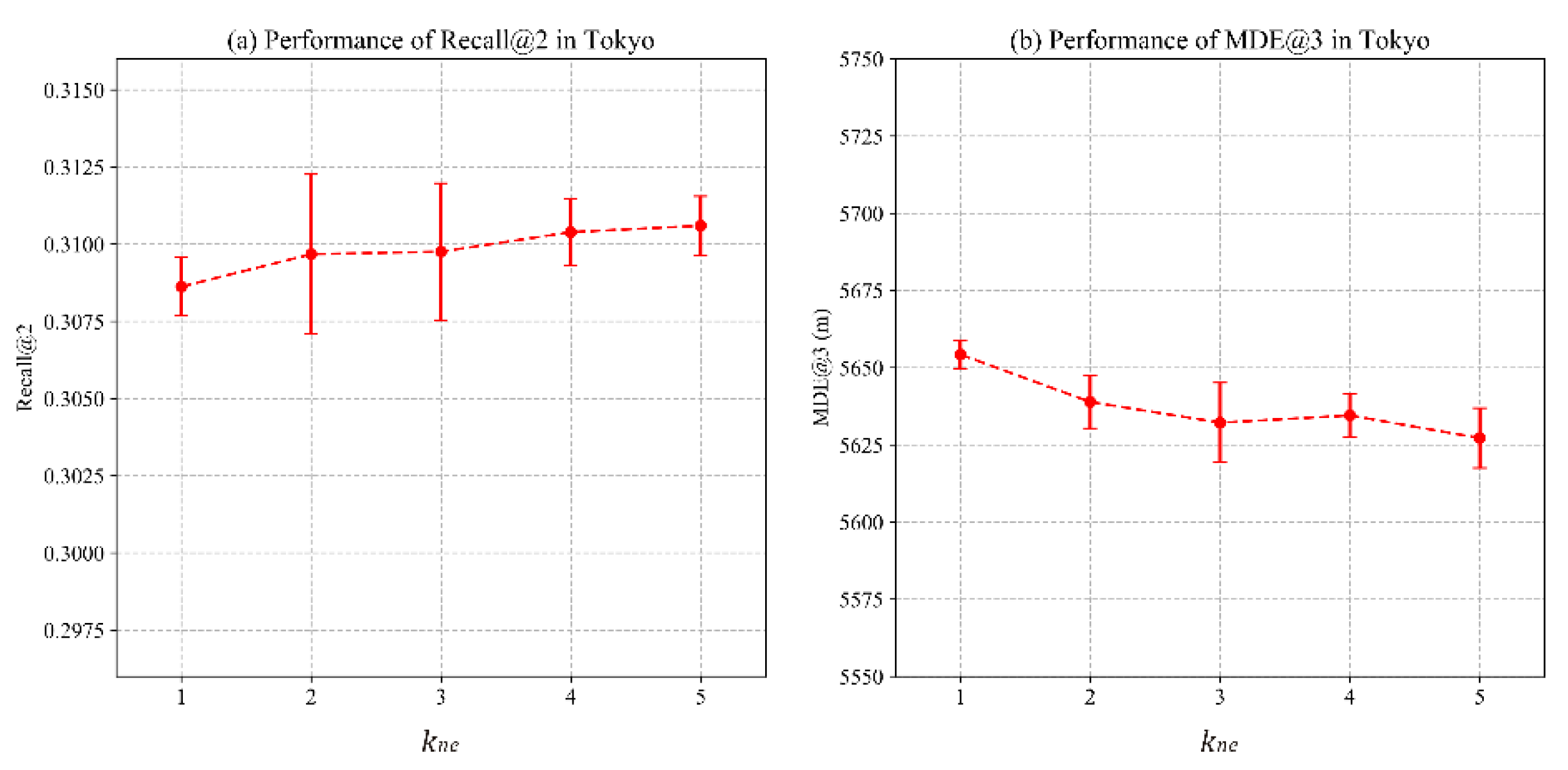
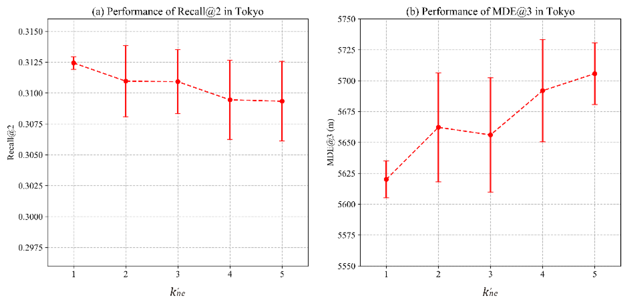
4.3. Parameter Sensitivity Analysis

In this section, we discuss how the value of the parameters affects the results. The major parameters include the number of dimensions f 1 and f 2 , the number of negative samples k n e and k n e , and learning rate η 1 and η 2 . We mainly use Recall@2 and MDE@3 to compare the performance. For each value of the parameters, we repeat the experiment three times and take the average results. We also tune the linear weight α as 0.5 temporarily to reduce the influence of different weights of the two components on the result.

4.3.1. Impact of Dimension

We first discuss the impact of the dimension number f 1 and f 2 . Figure 8 and Figure 9 show the line chart with error bars of the impact of f 1 and f 2 , respectively. We vary the value of f 1 from 10 to 50 with a step of 10, and that of f 2 from 40 to 100. When the value of f 1 from 10 to 20, Recall@2 value has increased significantly. However, the increase slows down and remains almost steady when f 1 value varies from 20 to 50. Similarly, when the number of f 2 reaches 70 or 80, the increase of Recall@2 value slows down, and even has a little fluctuation. The common trend is that while the number of dimensions increases, the performance improves, but the time cost also increases. The difference is that the value of f 2 does not influence the result as much as that of f 1 , but its influence to time cost is much larger than that of f 1 because the embedding v u i with f 2 dimension needs to be inner product with high-dimensional visual embeddings. Therefore, as analyzed above, we set the value of f 1 as 40 and f 2 as 60 in this paper.

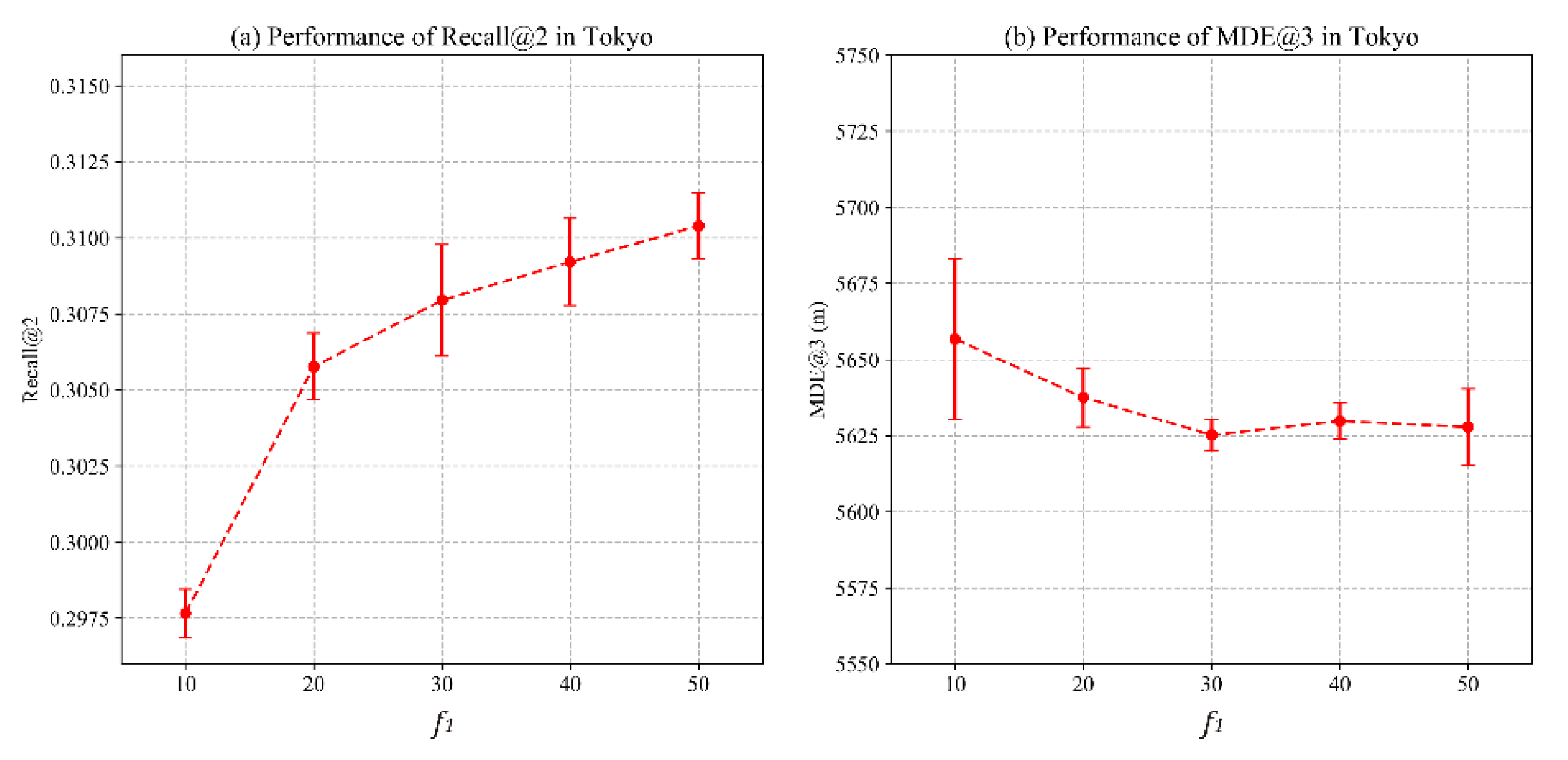
4.3.2. Impact of Negative Samples

The impact of negative samples is less discussed, compared to that of the dimension. Figure 10 and Figure 11 shows the impact of k n e and k n e , respectively. It seems that the negative sample number increase does not necessarily make the performance better: the performance of the two metrics get slightly better when k n e value increases, while the performance becomes even worser as k n e value increases. Nevertheless, the number of negative samples does not influence the result as much as that of dimension, and the overall performance can still remain satisfactory. Therefore, we obtain the value of k n e and k n e intuitively from the charts, which are set as 5 and 1, respectively.

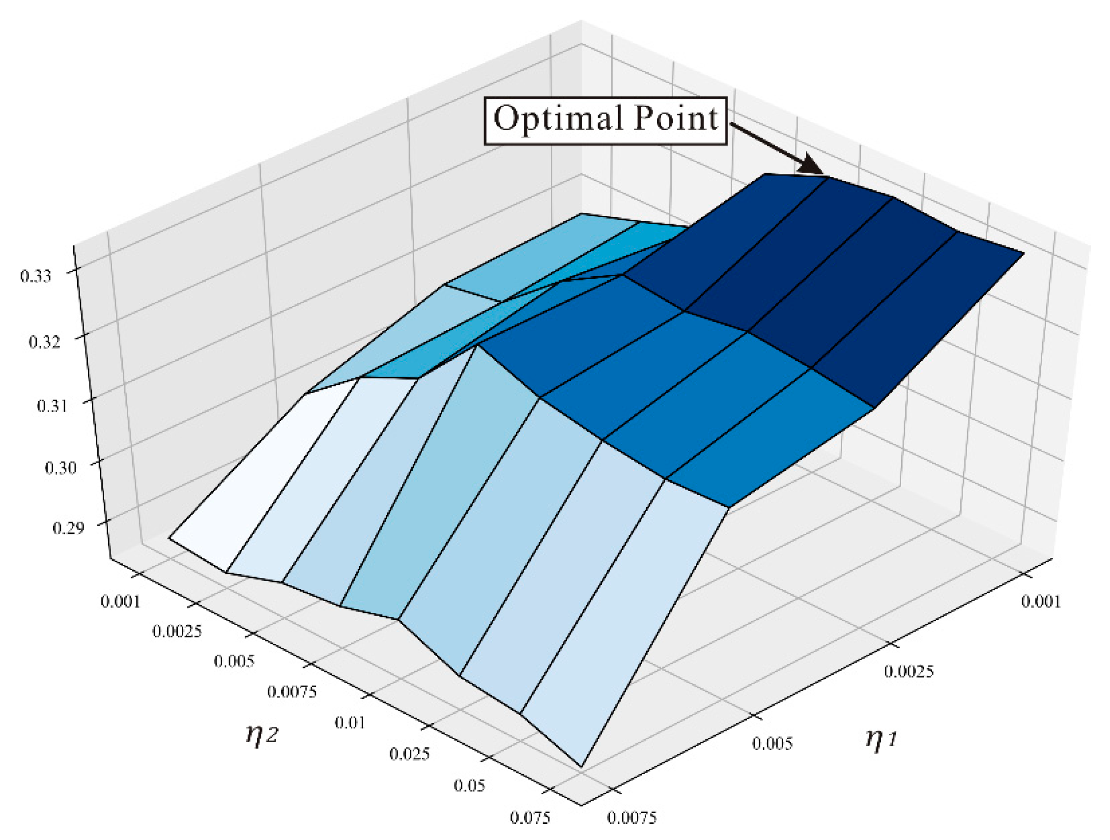
4.3.3. Impact of Learning Rate

η 1 and η 2 are the learning rates of S T and V part, respectively. Setting different learning rates for combined models has been tried in previous studies [19]. Figure 12 shows how the combination of η 1 and η 2 values influence the recall@2 value. In the experiment, we varied η 2 from 0.001 to 0.075, and η 1 from 0.001 to 0.0075 because we find that that STVE becomes drastically worse when η 1 is larger than 0.001. This may be because a too large learning rate leads to divergence. When η 1 is equal to 0.001, the Recall@2 value is generally high. Additionally, within the range from 0.001 to 0.01 of η 2 value, the overall result also gets better as the value increases. After η 2 value is larger than 0.01, the result remains steady. We select the value of η 1 and η 2 when they together achieve the optimal point, and the value of η 1 and η 2 is 0.001 and 0.01, respectively.

4.4. Component-Wise Study

We further explore how each component affects the performance as STVE is a combined model considering various factors. We split each component and compare their performance, and each component/model includes: (1) Only the spatial and temporal part S T (marked as “ST” in the following), i.e., α is set as 1 in Equation (14). (2) S T that removes the spatial distance constraint, i.e., α is set as 1 and select the negative samples randomly instead of selecting in the negative sample set outside the cutoff distance (marked as “T”). (3) Only the visual part V , i.e., α is set as 0 (marked as “V”). (4) The complete STVE model. Table 2 shows the result comparison between STVE and its components in the metrics of precision@2, recall@2, MDE@3, and MRR. Each component’s performance is not as good as that of the complete STVE model—a common result in combined models. Among these three components, ST’s gap between STVE is relatively small; followed by the T component. The V component performs worst when solely used, but after combining with the ST component, the overall performance improves compared to using ST. Additionally, fusing content information can also play an important role in solving the cold-start problem. The result shows that our STVE model can effectively improve recommendation accuracy compared with any single component.

4.5. Results for Cold-Start User

We briefly analyze how STVE performs in the cold-start issue. We assume the users who visited less than six tourist attractions to be the cold-start users and remove the other users. The number of the remaining trajectories is 659. Train STVE and five baseline methods with these remaining trajectories and further compare their performance in four metrics. As Figure 13 shows, our STVE model still obtains the best performance among these models, but its gap with other baseline models is larger. For instance, for all users in Figure 7, the MRR value difference between Geo-Teaser and UCF is 0.0792 and 0.2528, respectively, whereas, for cold-start users, the MRR value difference is 0.1531 and 0.3837, respectively. Additionally, the performance of VBPR in the former three metrics is not much different from FPMC-LR and is inferior to Geo-Teaser for all users, whereas for cold-start users, VBPR performs second to STVE. It may be because VBPR is a kind of content-based model, and the content-based model is not sensitive to the cold-start issue. Similarly, STVE fuses visual content based on the principle of VBPR and therefore obtains good performance in the cold-start issue. Another impressive result is that the difference between UCF and BPR-MF for cold-start users is smaller than that for all users. Take the MRR value as an example again; the difference between UCF and BPR-MF for all users is 0.0734, whereas that for cold-start users is 0.0381. It demonstrates that both memory- and model-based CF will be negatively affected by the cold-start issue when they do not fuse any content and contextual information.

5. Conclusions

In this paper, we propose a hybrid tourist attraction recommendation model that fuses spatial, temporal, and visual embeddings for Flickr-geotagged photos (STVE). In the preprocessing steps, we leverage a framework to automatically filter the noisy and redundant photos and select representative images of tourist attractions to extract visual embeddings as accurately as possible. To build the STVE model, we modify Skip-gram’s objective function and leverage Word2Vec’s negative sampling strategy to model the spatial and temporal factors. Then we use Matrix Factorization to fuse the tourist attractions’ visual embeddings and train with Visual Bayesian Personalized Ranking. We select Tokyo as the study area to evaluate our STVE model.
The comparison results show that our STVE model can relieve the low accuracy issue of content-based methods and the cold-start issue of CF-based methods. We also analyzed the sensitivity of the main parameters and explore how each component influences the recommendation results. The series of results demonstrate the superiority of STVE in providing a recommendation of high accuracy and provide us with further motivation to pursue our research. In future work, we will continue to improve our recommendation models by adding more contextual information (such as weather and season) and user attributes (such as age and gender). Furthermore, we will try to implement our model in web-based applications or other platforms for actual use.

Author Contributions

Conceptualization, Shanshan Han and Qingyun Du; Methodology, Shanshan Han and Dawei Gui; Software, Shanshan Han and Dawei Gui; Formal Analysis, Shanshan Han and Dawei Gui; Resources, Cuiming Liu; Data Curation, Shanshan Han and Dawei Gui; Writing—Original Draft Preparation, Shanshan Han, Dawei Gui and Qingyun Du; Writing—Review & Editing, Shanshan Han, Cuiming Liu and Keyun Chen; Visualization, Shanshan Han; Supervision, Cuiming Liu and Keyun Chen. All authors have read and agreed to the published version of the manuscript.

Funding

This research received no external funding.

Institutional Review Board Statement

Not applicable.

Informed Consent Statement

Not applicable.

Data Availability Statement

Publicly available datasets were analyzed in this study. This data can be found here: http://projects.dfki.uni-kl.de/yfcc100m/.

Acknowledgments

We thank YFCC100M for licensing the image dataset under a Creative Commons Attribution, and some images in these figures were clipped according to cartographic needs.

Conflicts of Interest

The authors declare no conflict of interest.

References

  1. Hendler, J. Web 3.0 Emerging. Computer 2009, 42, 111–113. [Google Scholar] [CrossRef]
  2. Rudman, R.; Bruwer, R. Defining Web 3.0: Opportunities and challenges. Electron. Libr. 2016, 34, 132–154. [Google Scholar] [CrossRef]
  3. World Travel & Tourism Council. Available online: https://www.wttc.org (accessed on 25 February 2020).
  4. World Tourism Organization. UNWTO Tourism Highlights, 2019th ed.; UNWTO: Madrid, Spain, 2018. [Google Scholar]
  5. Report of Global Independent Travel. 2017. Available online: http://www.mafengwo.cn/activity/sales_.report2017/index (accessed on 28 December 2019).
  6. Gao, Y.; Tang, J.; Hong, R.; Dai, Q.; Chua, T.S.; Jain, R. W2Go: A travel guidance system by automatic landmark ranking. In Proceedings of the 18th ACM international conference on Multimedia, Firenze, Italy, 25–29 October 2010; pp. 123–132. [Google Scholar]
  7. Zhou, X.; Xu, C.; Kimmons, B. Detecting tourism destinations using scalable geospatial analysis based on cloud computing platform. Comput. Environ. Urban Syst. 2015, 54, 144–153. [Google Scholar] [CrossRef]
  8. Rafsanjani, A.H.N.; Salim, N.; Aghdam, A.R.; Fard, K.B. Recommendation Systems: A review. Int. J. Comput. Eng. Res. 2013, 3, 47–52. [Google Scholar]
  9. Van Meteren, R.; Van Someren, M. Using content-based filtering for recommendation. In Proceedings of the Machine Learning in the New Information Age MLnet/ECML2000 Workshop, Barcelona, Spain, 30 May 2000; pp. 47–56. [Google Scholar]
  10. Schafer, J.B.; Frankowski, D.; Herlocker, J.; Sen, S. Collaborative Filtering Recommender Systems; Springer: Berlin/Heidelberg, Germany, 2007; pp. 291–324. [Google Scholar]
  11. Bao, J.; Zheng, Y.; Wilkie, D.; Mokbel, M.F. Recommendations in location-based social networks: A survey. GeoInformatica 2015, 19, 525–565. [Google Scholar] [CrossRef]
  12. Adomavicius, G.; Sankaranarayanan, R.; Sen, S.; Tuzhilin, A. Incorporating contextual information in recommender systems using a multidimensional approach. ACM Trans. Inf. Syst. 2005, 23, 103–145. [Google Scholar] [CrossRef] [Green Version]
  13. Renjith, S.; Sreekumar, A.; Jathavedan, M. An extensive study on the evolution of context-aware personalized travel recommender systems. Inform. Process. Manag. 2020, 57, 102078. [Google Scholar] [CrossRef]
  14. Rendle, S.; Freudenthaler, C.; Schmidt-Thieme, L. Factorizing personalized Markov chains for next-basket recommendation. In Proceedings of the 19th international conference on Architectural support for programming languages and operating systems; Association for Computing Machinery (ACM), Raleigh, NC, USA, 26–30 April 2010; pp. 811–820. [Google Scholar]
  15. Cheng, C.; Yang, H.; Lyu, M.R.; King, I. Where you like to go next: Successive point-of-interest recommendation. In Proceedings of the Twenty-Third International Joint Conference on Artificial Intelligence, Beijing, China, 3–9 August 2013. [Google Scholar]
  16. Feng, S.; Li, X.; Zeng, Y.; Chee, Y.M. Personalized ranking metric embedding for next new poi recommendation. In Proceedings of the Twenty-Fourth International Joint Conference on Artificial Intelligence, Buenos Aires, Argentina, 25–31 July 2015; pp. 2069–2075. [Google Scholar]
  17. Tang, J.; Qu, M.; Wang, M.; Zhang, M.; Yan, J.; Mei, Q. Line: Large-scale information network embedding. In Proceedings of the 24th International Conference on World Wide Web, New York, NY, USA, 18–22 May 2015; pp. 1067–1077. [Google Scholar]
  18. Xie, M.; Yin, H.; Wang, H.; Xu, F.; Chen, W.; Wang, S. Learning graph-based poi embedding for location-based recommendation. In Proceedings of the 25th ACM International on Conference on Information and Knowledge Management, Indianapolis, IN, USA, 24–28 October 2016; pp. 15–24. [Google Scholar]
  19. Zhao, S.; Zhao, T.; King, I.; Lyu, M.R. Geo-teaser: Geo-temporal sequential embedding rank for point-of-interest recom-mendation. In Proceedings of the 26th International Conference on World Wide Web Companion, Geneva, Switzerland, 3–7 April 2017; pp. 153–162. [Google Scholar]
  20. Ye, M.; Yin, P.; Lee, W.-C.; Lee, D.-L. Exploiting geographical influence for collaborative point-of-interest recommendation. In Proceedings of the 34th International ACM SIGIR Conference on Research and Development in Information—SIGIR ’11, Beijing, China, 25–29 July 2011; pp. 325–334. [Google Scholar]
  21. Zhang, Z.; Zou, C.; Ding, R.; Chen, Z. VCG: Exploiting visual contents and geographical influence for Point-of-Interest recommendation. Neurocomputing 2019, 357, 53–65. [Google Scholar] [CrossRef]
  22. Cheng, C.; Yang, H.; King, I.; Lyu, M.R. Fused matrix factorization with geographical and social influence in location-based social networks. In Proceedings of the Twentysixth AAAI conference on artificial intelligence, Toronto, ON, Canada, 22 July 2012; pp. 17–23. [Google Scholar]
  23. Lian, D.; Zhao, C.; Xie, X.; Sun, G.; Chen, E.; Rui, Y. GeoMF: Joint geographical modeling and matrix factorization for point-of-interest recommendation. In Proceedings of the 20th ACM SIGKDD International Conference on Knowledge Discovery and Data Mining, New York, NY, USA, 24–27 August 2014; pp. 831–840. [Google Scholar]
  24. He, J.; Li, X.; Liao, L.; Song, D.; Cheung, W.K. Inferring a personalized next point-of-interest recommendation model with latent behavior patterns. In Proceedings of the Thirtieth AAAI Conference on Artificial Intelligence, Phoenix, AZ, USA, 12–17 February 2016; pp. 137–143. [Google Scholar]
  25. Gao, H.; Tang, J.; Huan, L.; Liu, H. Exploring temporal effects for location recommendation on location-based social networks. In Proceedings of the 7th ACM Conference on Recommender Systems, Hong Kong, China, 12–17 October 2013; pp. 93–100. [Google Scholar]
  26. Yuan, Q.; Cong, G.; Ma, Z.; Sun, A.; Thalmann, N.M. Time-aware point-of-interest recommendation. In Proceedings of the 36th international ACM SIGIR Conference on Research and Development in Information Retrieval—SIGIR ’13, Dublin, Ireland, 28 July–1 August 2013; pp. 363–372. [Google Scholar]
  27. Shi, Y.; Serdyukov, P.; Hanjalic, A.; Larson, M. Personalized landmark recommendation based on geotags from photo sharing sites. In Proceedings of the Fifth International AAAI Conference on Weblogs and Social Media, Barcelona, Spain, 17–21 July 2011. [Google Scholar]
  28. Memon, I.; Chen, L.; Majid, A.; Lv, M.; Hussain, I.; Chen, G. Travel recommendation using geo-tagged photos in social media for tourist. Kluw. Commun. 2015, 80, 1347–1362. [Google Scholar] [CrossRef]
  29. Chen, Y.-Y.; Cheng, A.-J.; Hsu, W.H. Travel Recommendation by Mining People Attributes and Travel Group Types from Community-Contributed Photos. IEEE Trans. Multimed. 2013, 15, 1283–1295. [Google Scholar] [CrossRef]
  30. Subramaniyaswamy, V.; Vijayakumar, V.; Logesh, R.; Indragandhi, V. Intelligent Travel Recommendation System by Mining Attributes from Community Contributed Photos. Procedia Comput. Sci. 2015, 50, 447–455. [Google Scholar] [CrossRef] [Green Version]
  31. AlBanna, B.; Sakr, M.; Moussa, S.; Moawad, I. Interest Aware Location-Based Recommender System Using Geo-Tagged Social Media. ISPRS Int. J. Geo.-Inf. 2016, 5, 245. [Google Scholar] [CrossRef] [Green Version]
  32. Liu, Z.; Zhou, X.; Shi, W.; Zhang, A. Recommending attractive thematic regions by semantic community detection with multisourced VGI data. Int. J. Geogr. Inf. Sci. 2019, 33, 1520–1544. [Google Scholar] [CrossRef]
  33. Cao, L.; Luo, J.; Gallagher, A.; Jin, X.; Han, J.; Huang, T.S. A worldwide tourism recommendation system based on geotagged web photos. In Proceedings of the 2010 IEEE International Conference on Acoustics, Speech and Signal Processing, Dallas, TX, USA, 14–19 March 2010; pp. 2274–2277. [Google Scholar]
  34. Jiang, K.; Wang, P.; Yu, N. ContextRank: Personalized tourism recommendation by exploiting context information of geotagged web photos. In Proceedings of the 2011 Sixth International Conference on Image and Graphics, Hefei, China, 12–15 August 2011; pp. 931–937. [Google Scholar]
  35. Wang, S.; Wang, Y.; Tang, J.; Shu, K.; Ranganath, S.; Liu, H. What your images reveal: Exploiting visual contents for point-of-interest recommendation. In Proceedings of the 26th International Conference on World Wide Web, Perth, Australia, 3–7 April 2017; pp. 391–400. [Google Scholar]
  36. Thomee, B.; Shamma, D.A.; Friedland, G.; Elizalde, B.; Ni, K.; Poland, D.; Li, L.J. YFCC100M: The new data in multimedia research. Commun. ACM 2016, 59, 64–73. [Google Scholar] [CrossRef]
  37. Menk, A.; Sebastia, L.; Ferreira, R. Recommendation Systems for Tourism Based on Social Networks: A Survey. arXiv 2019, arXiv:1903.12099. [Google Scholar]
  38. Survey Concerning Visitors to Tokyo in 2018. Available online: http://www.metro.tokyo.jp/english/topics/.2019/0828_01.html (accessed on 20 December 2019).
  39. Han, S.; Ren, F.; Du, Q.; Gui, D. Extracting Representative Images of Tourist Attractions from Flickr by Combining an Improved Cluster Method and Multiple Deep Learning Models. ISPRS Int. J. Geo.-Inf. 2020, 9, 81. [Google Scholar] [CrossRef] [Green Version]
  40. Wang, J.; Song, Y.; Leung, T.; Rosenberg, C.; Wang, J.; Philbin, J.; Chen, B.; Wu, Y. Learning Fine-Grained Image Similarity with Deep Ranking. In Proceedings of the 2014 IEEE Conference on Computer Vision and Pattern Recognition, Columbus, OH, USA, 23–28 June 2014; pp. 1386–1393. [Google Scholar]
  41. Liu, W.; Anguelov, D.; Erhan, D.; Szegedy, C.; Reed, S.; Fu, C.-Y.; Berg, A.C. Ssd: Single shot multibox detector. In Proceedings of the European Conference on Computer Vision, Amsterdam, The Netherlands, 11–14 October 2016; pp. 21–37. [Google Scholar]
  42. Li, F.L.; Fergus, R.; Perona, P. Learning generative visual models from few training examples: An incremental Bayesian approach tested on 101 object categories. Comput. Vis. Image Und. 2007, 106, 59–70. [Google Scholar]
  43. Zhou, B.; Lapedriza, A.; Khosla, A.; Oliva, A.; Torralba, A. Places: A 10 Million Image Database for Scene Recognition. IEEE Trans. Pattern Anal. Mach. Intell. 2018, 40, 1452–1464. [Google Scholar] [CrossRef] [Green Version]
  44. He, R.; McAuley, J. VBPR: Visual Bayesian Personalized Ranking from implicit feedback. In Proceedings of the Thirtieth AAAI Conference on Artificial Intelligence, Phoenix, AZ, USA, 12–17 February 2016; pp. 144–150. [Google Scholar]
  45. Yao, D.; Zhang, C.; Huang, J.; Bi, J. Serm: A recurrent model for next location prediction in semantic trajectories. In Proceedings of the 2017 ACM on Conference on Information and Knowledge Management, Singapore, 6–10 November 2017; pp. 2411–2414. [Google Scholar]
  46. Adomavicius, G.; Tuzhilin, A. Toward the next generation of recommender systems: A survey of the state-of-the-art and possible extensions. IEEE Trans. Knowl. Data Eng. 2005, 17, 734–749. [Google Scholar] [CrossRef]
  47. Majid, A.; Chen, L.; Chen, G.; Mirza, H.T.; Hussain, I.; Woodward, J. A context-aware personalized travel recommendation system based on geotagged social media data mining. Int. J. Geogr. Inf. Sci. 2013, 27, 662–684. [Google Scholar] [CrossRef]
Figure 1. The overall framework of the study.
Ijgi 10 00020 g001
Figure 2. The spatial distribution of geotagged photos used in the study (in Tokyo, Japan).
Ijgi 10 00020 g002
Figure 3. Cluster results of some tourist attractions in Tokyo.
Ijgi 10 00020 g003
Figure 4. The construction of the user visiting trajectory.
Ijgi 10 00020 g004
Figure 5. The STVE’s structure and its connection with the preprocessing steps.
Ijgi 10 00020 g005
Figure 6. Tourist attraction visiting patterns at different hours within one day in the study area.
Ijgi 10 00020 g006
Figure 7. The performance comparison among the STVE and other models on: (a) Precision, (b) Recall, (c) Mean Reciprocal Rank, and (d) Mean Distance Error.
Ijgi 10 00020 g007
Figure 8. The impact of f1’s value changes on (a) Recall@2, (b) MDE@3.
Ijgi 10 00020 g008
Figure 9. The impact of f2’s value changes on (a) Recall@2, (b) MDE@3.
Ijgi 10 00020 g009
Figure 10. The impact of kne’s value changes on (a) Recall@2, (b) MDE@3.
Ijgi 10 00020 g010
Figure 11. The impact of kne’s value changes on (a) Recall@2, (b) MDE@3.
Ijgi 10 00020 g011
Figure 12. The impact of η 1 and η 2 ’s value changes on Recall@2.
Ijgi 10 00020 g012
Figure 13. The performance comparison among the STVE and other models for cold-start users on: (a) Precision, (b) Recall, (c) Mean Reciprocal Rank, and (d) Mean Distance Error.
Ijgi 10 00020 g013
Table 1. Notation description.
NotationDescription
T the training dataset for all users in the study area
u i , l j a user i and a tourist attraction j
l k , l k + 1 the k -th and ( k + 1 ) -th tourist attractions visited by the user i
t k + 1 the time slot of the user i to visit his/her k -th attractions
v l k , v l k + 1 the f 1 -dimensional embedding representations of l k and l k + 1
v t k + 1 the f 1 -dimensional embedding representations of t k + 1
v u i the f 1 -dimensional embedding representations of user i
e ¯ l j the visual embeddings of representative images for the attraction j
k n e , k n e the number of negative samples for spatial-temporal embeddings and visual embeddings
l n e , l n e the negative sample attractions for spatial-temporal embeddings and visual embeddings
f 1 the number of dimensions for v l k , v l k + 1 and v t k + 1 .
f 2 the number of dimensions for v u i
f e the number of dimensions for visual embeddings
W u l f 2 × f e embedding matrix
Table 2. The result comparison between spatial, temporal, and visual embeddings (STVE) and its components.
Component/
Model
Evaluation Metrics
P@2R@2MDE@3MRR
ST0.14950.30455925.62130.3275
T0.14640.29786893.42330.3169
V0.09160.18328119.15030.2395
STVE0.15570.31145660.69620.3378
Publisher’s Note: MDPI stays neutral with regard to jurisdictional claims in published maps and institutional affiliations.

