Analysis of Differences in the Spatial Distribution among Terrestrial Mammals Using Geodetector—A Case Study of China

Abstract

The survival and distribution of animals cannot be separated from a certain environment. How patterns in mammalian species depend on the environment remain unclear. This study incorporating spatial data on climate, precipitation, topography, and vegetation quantitatively analyzed the influence of specific geographical factors on the spatial distribution of terrestrial mammalian richness using the Geodetector model. We used the spatial analysis method of geographical information systems (GIS), separating the mammalian distribution of 621 species into 10 by 10 km grids to measure spatial richness. Our results showed that there were significant spatial differences in terrestrial mammalian richness in China. There was a low richness in the east and west, but high richness in the south. Individual factor detection results showed that annual precipitation (AP) and the minimum temperature of the coldest month (MTCM) were the dominant factors affecting the spatial pattern of mammal richness in China. Patterns in the distribution of species richness had distinct characteristics for different mammalian orders and were influenced by different environmental factors. The richness distribution of most orders was mainly affected by MTCM and AP. Interactive detection results showed that interacting factors in pairs play much bigger roles in the spatial distribution of species richness than individual factors. The synergistic effect of elevation with AP and MTCM best explained the distribution differences of species richness. We found that the Geodetector model is a valuable tool, hoping to be more widely used in biogeography.

1. Introduction

The survival and distribution of any animal cannot be separated from a certain environment. The negative consequences of human activities restrict the development of resources and the environment, consequently causing detrimental impacts on the natural habitat [1]. Many species have been annihilated or are in a state of imminent danger. However, how patterns in the distribution of species depend on the environment remain unclear.

How species are distributed is the combined effect of abiotic factors and biotic interactions [2,3,4,5]. Notably, many scholars have proposed hypotheses to explain the mechanisms of influencing patterns in the geographical distribution of species. Such hypotheses include the productivity hypothesis [6,7], ambient energy hypothesis [8,9], environmental stability hypothesis [10,11], water–energy dynamic hypothesis [12,13], freezing tolerance hypothesis [13,14], habitat heterogeneity hypothesis [15], and historical hypothesis [16]. These hypotheses reveal different forms of energy influencing the spatial patterns of animals from different perspectives.

Landscape, climate, topography, and social processes may affect the distribution of animals [4,17]. There have been many available methods in estimating the relationship between the geographical distribution of species and environment variables. Correlation analyses are used to test consistency in the geographical patterns of diversity for different taxonomic groups [18]. Regression models are often used for quantifying the relationship between one variable and others upon which it depends [19]. In particular, generalized linear models (GLMs), including linear regression, logistic regression, and Poisson regression, are suitable for analyzing nonlinear relationships between species and environmental variables [20]. With the development of computer technology, complex models such as machine learning have a strong predictive ability in simulating distributions of species, which can handle complex response relations [20,21,22,23,24,25]. Classification and regression tree (CART) can reveal the interaction between complex predictors [20]. Multivariate regression trees (MRTs) can be used to explore and predict relationships between species data and environmental characteristics [21]. Random forests or boosted regression trees (BRTs) are often used to explore and predict which environmental factors influence the distribution of animals [22,23]. Ecological niche models also identify the importance of the variables, provide response curves for each variable, and provide a potential distribution range according to the environmental variables associated with species occurrence records [24,25].

Geodetector is a new statistical model to analyze geographical phenomena with spatial stratified heterogeneity, which consists of four detectors [26]: factor, ecological, interaction, and risk. The factor detector can reveal the relative importance or influence intensity among these key factors without any assumptions or limitations compared to the traditional statistical methods [26,27,28]. The ecological detector identifies the difference in impact between two explanatory variables [26,28]. The interaction detector can also analyze the interactions between factors that influence response variables [26,28]. The risk detector analyzes whether the mean of the attributes between the two subareas of factors is significantly different [26,28]. Geodetector can explore more comprehensively the determinants of stratified heterogeneity of dependent variables from four aspects. It has been utilized in numerous studies, including public health [28], land use [29], and ecological environment [30], and it has been gradually adopted for the research of animal-related fields. Shen et al. [31] used the Geodetector model to detect the suitability of grasshopper habitat in steppe habitats of Inner Mongolia. Fan et al. [32] used Geodetector software to study the influence of habitat factors on the distribution pattern of Spermophilus dauricus in the Manchuria City of China. Chen et al. [33] analyzed the relationships among the biogeographic patterns of the α-diversity of mangrove mollusks and environmental factors and spatial variables by using the Geodetector software. Liu et al. [34] assessed the influence of soil, land use, vegetation, and normalized difference vegetation index (NDVI) layers on the distribution of rodent density using Geodetector. Liu et al. [35,36] tested the q statistic by Geodetector to avoid the possible confounding caused by spatial stratified heterogeneity.

In China, quantitative studies of the mechanisms influencing the formation of mammalian distribution patterns remain limited due to the limited availability of macrolevel data. In this paper, we aim to present possibilities of using the Geodetector by ecologists, demonstrating its use in an analysis of relationships between mammalian distribution and environments. We used the Geodetector model combined with geospatial data and recent animal taxonomic data to explore the intrinsic relationship between the spatial pattern of terrestrial mammalian richness and environmental factors. The Geodetector model is based on spatial differentiation analysis by combining spatial overlay technology of geographical information systems (GIS). Our study systematically analyzed the relationship between different geographical environmental factors influencing the distribution of species richness to more accurately understand the extent to which species distributions are affected by environmental factors. Our analysis was expected to provide an important reference and scientific basis for the conservation policy of species diversity in China.

2. Materials and Methods

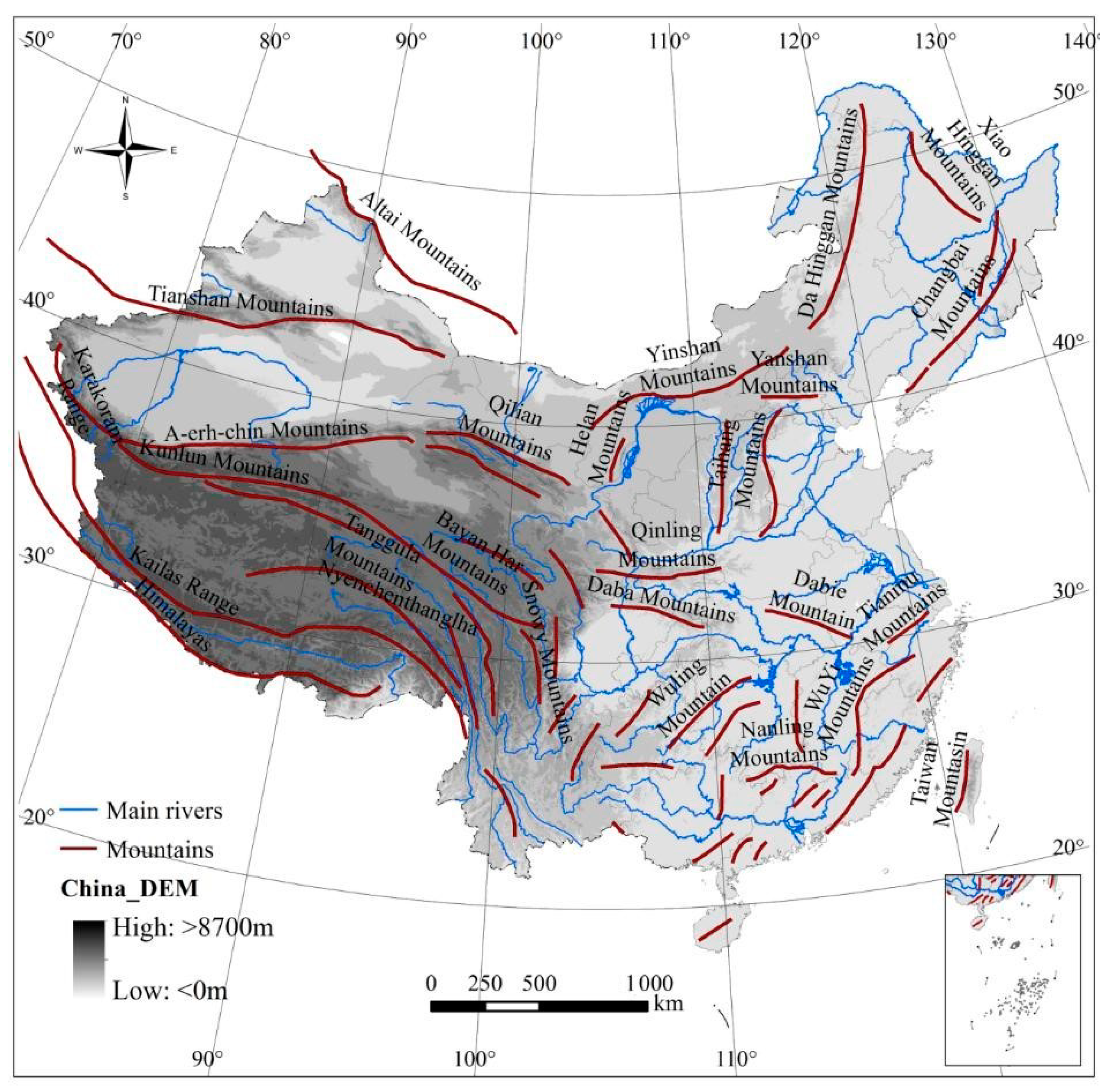
2.1. Study Area

The study encompassed the entire area of China (9.6 million km²; 73°29′ east (E)–135°2′ E, 3°31′ north (N)–53°33′ N), see Figure 1. From east to west, the country extends about 5200 km; from north to south, it spans about 5500 km. The country is characterized by diverse terrain, different climate types, and complex natural conditions. It is the diversity of habitat environments that leads to incredible species abundance. China is one of the countries with the richest biodiversity globally [37]. The geological environment has been subject to events, including tectonic movement and the uplifting of the Qinghai–Tibetan Plateau, which has resulted in clear regional differences to the natural environment and has influenced the geographical pattern in the distribution of animals [38].

2.2. Data Materials

2.2.1. Distribution Data of Terrestrial Mammals

Data on the distribution of mammals were represented as polygons, from China’s Mammal Diversity and Geographic Distribution [39], which supplements and revises basic information in the species list. The published database contained terrestrial mammals comprising 11 orders and 625 species. For this study, humans and three locally extinct species (Sumatran rhinoceros, Javan rhinoceros, Indian rhinoceros) were excluded. The final analysis included 11 orders and 621 species. Preprocessing revealed that species distribution maps exhibit uniform Albers equal-area conic projection.

The distribution ranges of terrestrial mammals overlap in space. We divided the whole study area into grids with 10 by 10 km to quantify the distribution patterns of terrestrial mammals on the grid scale. We superimposed the distribution ranges of 621 terrestrial mammals using multilayer overlap statistics of GIS. They were recorded as “1” and “0” by counting the presence or absence of mammals in each 10 × 10 km grid. All individual species in each grid were added up to represent the species richness. The individual species within each taxonomic category per grid were as the richness of that particular taxon. A total of 94,860 grids were used for the analysis.

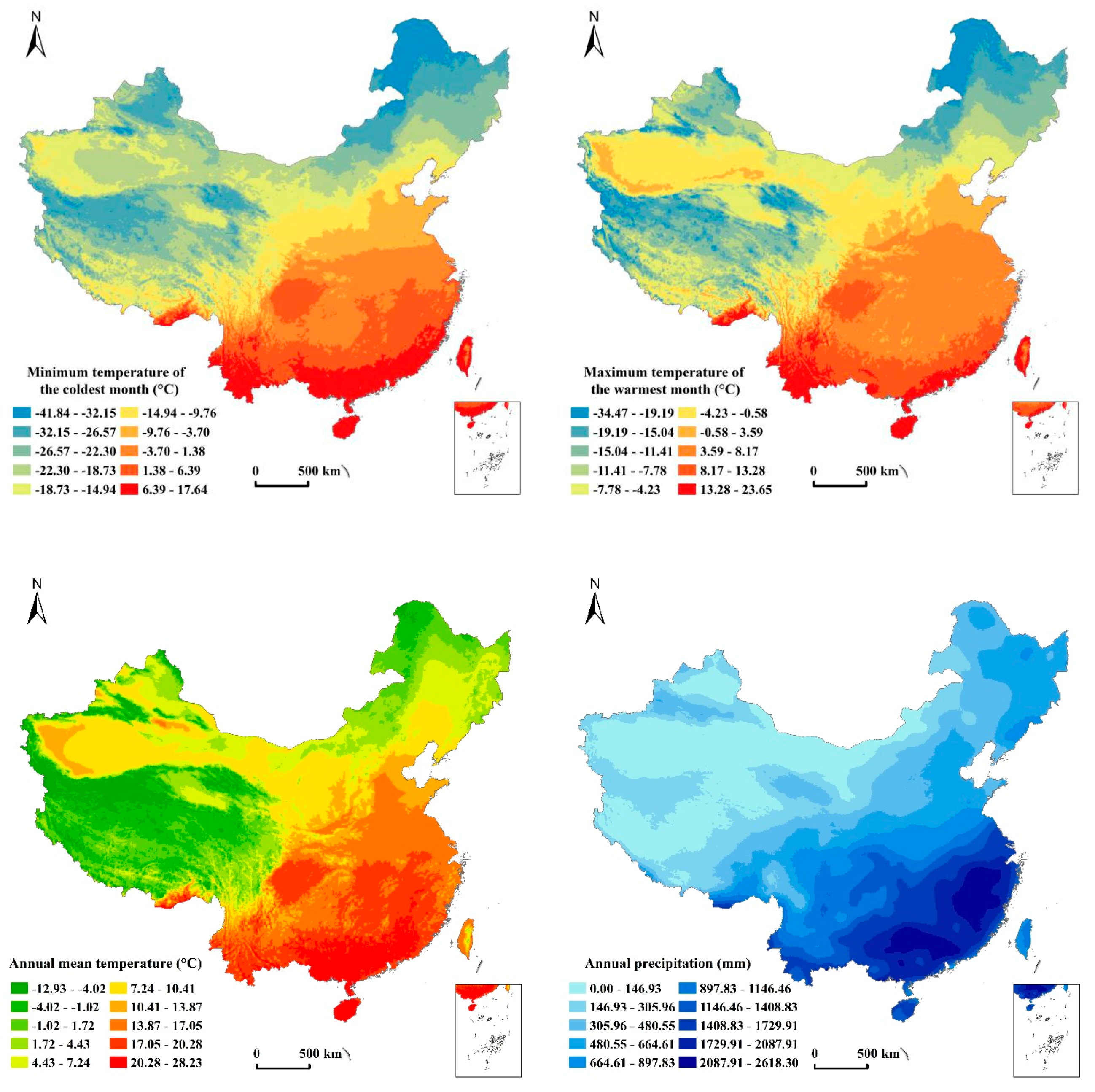
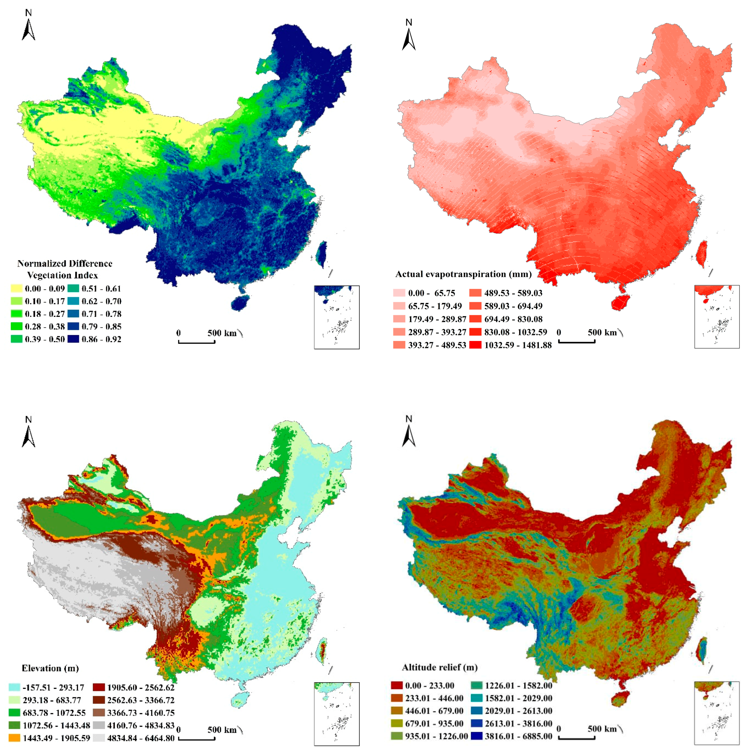
2.2.2. Data Resources of Environmental Factors

To explore how specific factors of the natural environment affect mammalian distribution in China, we selected 11 variables as environmental factors according to primary explanatory variables among hypotheses. The minimum temperature of the coldest month (MTCM) and maximum temperature of the warmest month (MTWM) reflect the freezing tolerance hypothesis [13,14]. The MTCM and MTWM were obtained from 1 km monthly temperature datasets for China from 2012 to 2014 of the National Earth System Science Data Center, National Science and Technology Infrastructure of China (http://www.geodata.cn). Annual mean temperature (AMT) is a natural factor representing the environmental heat hypothesis [40]. Annual precipitation (AP), normalized difference vegetation index (NDVI), and actual evapotranspiration (AET) reflect the productivity level of the region [41,42]. AMT was obtained from the annual average temperature dataset of China in 2015. AP was obtained from the annual precipitation data set of China in 2015. NDVI was obtained from the spatial distribution dataset of the normalized difference vegetation index of China in 2015. The datasets were obtained from the Data Center for Resources and Environmental Sciences, the Chinese Academy of Sciences (RESDC) (http://www.resdc.cn/DOI). The actual evapotranspiration was derived from the terrestrial evapotranspiration dataset across China in 2015. The dataset was provided by the National Tibetan Plateau Data Center (http://data.tpdc.ac.cn). Elevation (Ele), altitude relief (AR), soil type (ST), geomorphic type (GT), and land-use type (LT) represent habitat heterogeneity [43]. The digital elevation model with a spatial resolution of 30 m was derived from Aster GDEM. Soil type was derived from the distribution data of 1:1 million soil types in China, which consist of 13 soil orders. Geomorphic type data were derived from the spatial distribution dataset of 1:1 million geomorphic types in China, which have 8 categories. Land-use data were obtained from the remote sensing monitoring methods of land-use/cover changes of China in 2015, which have 8 categories. The datasets were provided by the Data Center for Resources and Environmental Sciences, the Chinese Academy of Sciences (RESDC) (http://www.resdc.cn). All maps of environmental factors were clipped and transformed uniform Albers equal-area conic projection and converted to grid squares, as well as joining the corresponding species distribution data. Due to the analysis being done in grids of 10 × 10 km, the information from the original layers was transformed into the resolution of 10 × 10 km. The MTCM, MTWM, AMT, AP, NDVI, AET, and Ele were the average of corresponding variables in each grid cell. Altitude relief (AR) was the height difference between the highest point and the lowest point in each grid. The Geodetector model uses categorical variables rather than numerical. Here, we converted numerical factors to categorial factors according to the algorithm of Natural Breaks [44], which is a classification method to divide similar values into one class and maximize the difference between classes [45]. We classified the values of eight numerical variables into 10 classes (shown in Supplementary Materials Table S1). According to the area-dominant method, the types of categorical variables with the largest coverage area were selected as the types for each grid cell. The spatial distributions of classifications for 11 variables are shown in Figure 2.

2.3. Methods

Spatial stratification heterogeneity (SSH) is one of the basic characteristics of geographical phenomena, which refers to the difference of a certain attribute value in different types or regions. Spatial data tend to be considerably more heterogeneous when the size of data becomes large [27]. Geodetector is a novel tool that utilizes spatial attributes to measure SSH, which consists of four detectors [26].

The factor detector in the Geodetector models focuses on the heterogeneity between the factor attributes. The extent to which factor X is detected explains the spatial differentiation of attribute Y. Measured with the q-statistic, it is expressed as follows [27]:

$$q=1-\frac{1}{N{\sigma }^2}{\displaystyle {\sum }_{h=1}^L{N}_h{\sigma }_h{}^2}=1-\frac{SSW}{SST}$$

(1)

$$SSW={\displaystyle {\sum }_{h=1}^L{N}_h{\sigma }_h{}^2}$$

(2)

$$SST=N{\sigma }^2$$

(3)

where h is the strata of variable Y or factor X (h = 1, 2, …, L). N_h and N are the unit numbers of layer h and the whole area. σ_h² and σ² are the variances of Y in layer h and the whole area. SSW and SST represent the sum of variance within the layer and the total variance of the whole area. A larger value of q denotes a more obvious spatial heterogeneity of Y and a stronger explanatory power of factor X to variable Y, q ∈ [0, 1].

The ecological detector compares whether there is a significant difference between the two factors on the spatial distribution of attribute Y, measured by the F-statistic.

$$F=\frac{N_{X1}(N_{X2}-1){SSW}_{X1}}{N_{X2}(N_{X1}-1){SST}_{X2}}$$

(4)

$${SSW}_{X1}={\displaystyle {\sum }_{h=1}^{L1}{N}_h{\sigma }_h{}^2}$$

(5)

$${SSW}_{X2}={\displaystyle {\sum }_{h=1}^{L2}{N}_h{\sigma }_h{}^2}$$

(6)

N_X1 and N_X2 represent sample sizes of the two factors X₁ and X₂, respectively; L₁ and L₂ represent the number of layers of X₁ and X₂, respectively, where the null hypothesis H₀ is SSW_X1= SSW_X2. If H₀ is rejected at the level of significance of α, this indicates that there is a significant difference in the effect of the two factors on the spatial distribution of Y.

The interaction detector investigates the general interaction between different explanatory risk factors X_S to a dependent variable Y. It investigates whether the influence of factors X_S on variable Y are independent and whether they work together to increase or weaken the explanatory power of the Y. First, the q values of the two factors X₁ and X₂ for Y are calculated separately: q(X₁) and q(X₂). The q value of their interactions is then calculated (by superimposing the new polygon distribution formed by the tangent of the two layers X₁ and X₂): q(X₁∩X₂). Then, q(X₁), q(X₂), and q(X₁∩X₂) are compared. If the q(X₁∩X₂) is less than the minimum of q(X₁) and q(X₂), the result is nonlinear weakened. If the q(X₁∩X₂) is between q(X₁) and q(X₂), the result is univariate nonlinear weaken. If the q(X₁∩X₂) is greater than the maximum of q(X₁) and q(X₂) and less than their sum, it is bivariate enhanced. If the q(X₁∩X₂) is the sum of q(X₁) and q(X₂), X₁ and X₂ are independent. If the q(X₁∩X₂) is the maximum value, it is nonlinear enhanced.

The risk detector can give the average Y in each subarea of a factor X. It uses the t statistic testing to determine whether the mean of the attributes between the two subareas is significantly different.

$$t_{\overline{y}h = 1 - {\overline{y}}_h = 2}=\frac{{\overline{Y}}_{h = 2}-{\overline{Y}}_{h = 2}}{\sqrt{{}^{{}^{\left[\frac{\mathrm{Var}({\overline{Y}}_{h = 1})}{n_{h = 1}}+\frac{\mathrm{Var}({\overline{Y}}_{h = 2})}{n_{h = 2}}\right]}}}}$$

(7)

where ${\overline{Y}}_h$ is the mean value of the attribute in layer h, n_h represents the number of samples in layer h, and Var is the variance. The statistic t approximately obeys the Student’s t distribution [46]. The calculation method of degrees of freedom is

$$df=\frac{\frac{\mathrm{Var}({\overline{Y}}_{h = 1})}{n_{h = 1}}+\frac{\mathrm{Var}({\overline{Y}}_{h = 2})}{n_{h = 2}}}{\frac{1}{n_{h = 1}-1}{\left[\frac{\mathrm{Var}({\overline{Y}}_{h = 1})}{n_{h = 1}}\right]}^2+\frac{1}{n_{h = 2}-1}{\left[\frac{\mathrm{Var}({\overline{Y}}_{h = 2})}{n_{h = 2}}\right]}^2}$$

(8)

where the null hypothesis H₀ is ${\overline{Y}}_{h = 1}={\overline{Y}}_{h = 2}$. If H₀ is rejected at the level of significance of α, there is a significant difference in the mean value of attributes between the two subareas [46].

3. Results

3.1. Influencing Factors on the Spatial Distribution of Terrestrial Mammalian Richness

Terrestrial mammals were widely distributed throughout the provinces of China (Figure 3). Noticeable spatial heterogeneity in mammalian distribution was detected in China, with low richness in the east, west, and north, but high richness in the south. Southern China, especially the Hengduan Mountains in Yunnan Province, supported the greatest richness in terrestrial mammalian species. On the contrary, the species richness was low in western and eastern China. Mammalian richness was lowest, with few species, in northern China.

The factor detector in the Geodetector models could test how environmental factors explained the spatial distribution of terrestrial mammal richness in China. The powers of determinant values (q) of 11 factors at the 5% significant level (p < 0.05) were calculated using the factor detector (

Table 1. Association of each environmental factor with species richness (q values).

	AP	MTCM	MTWM	AET	NDVI	ST	LT	AMT	Ele	GT	AR
q-statistic	0.57	0.53	0.47	0.44	0.42	0.40	0.37	0.37	0.19	0.16	0.15
p-value	0.00	0.00	0.00	0.00	0.00	0.00	0.00	0.00	0.00	0.00	0.00
Effect direction	+	+	+	+	+	+	−	+	−	+	+

Notes: significance level, p < 0.05. “+” and “−” stand for the positive and negative correlation between driving factor and species richness according to Pearson correlation analysis.

). The q values of environmental factors were sorted in the order AP > MTCM > MTWM > AET > NDVI > ST > LT > AMT > Ele > GT > AR. We used the ecological detector to show that there were significant differences in the effects of various environmental factors on the distribution of species richness.

AP had a q value of 0.57, revealing a significant impact on the distribution of mammal richness in China. The relatively high q values of MTCM indicated that there is a remarkable positive association between MTCM and mammal richness. MTWM contributed a rather significant positive impact on mammal richness compared to other factors, with q statistics as high as 47% (Table 1). The q values of AET showed the influence of actual evapotranspiration on mammal richness distributions, meaning that AET can explain about 44% of the mammal richness pattern. NDVI was the leading factor affecting the distribution of mammalian richness in China, accounting for 42% of the variation on mammal richness. The soil type (ST) was the key factor impacting mammal richness, which explained 40% of the variation of mammalian richness distribution. The effect of LT (land-use type) was secondary on the distribution of terrestrial mammal richness, explaining 37% of mammal richness variation. It was found that AMT plays a key role in mammal richness distribution. The explanatory power of AMT was 37%, which indicates that AMT largely contributes to the distribution of mammal richness. The elevation was positively and weakly correlated with mammal richness, with q statistics of 19%, whereas the elevation posed a negative effect on mammalian richness. Geomorphic type (GT) and altitude relief (AR) exerted relatively weak effects on mammal richness distribution, explaining 16% and 15% of the variance on mammalian richness respectively.

The interaction detector identified the interaction between pairs of environmental factors and tested whether two environmental variables work individually or interact with each other. If they interacted, the effect was enhanced or weakened. The interactions of each paired factor at a 5% explanatory power level are shown in

Table 2. Interaction of pairs of environmental factors (q values) on species richness.

	q(X2)	0.57	0.53	0.47	0.44	0.42	0.40	0.37	0.37	0.19	0.16	0.15
q(X1)	q(X1 ∩ X2)	AP	MTCM	MTWM	AET	NDVI	ST	LT	AMT	Ele	GT	AR
0.57	AP		bi-E	bi-E	bi-E	bi-E	bi-E	bi-E	bi-E	non-E	bi-E	bi-E
0.53	MTCM	0.66		bi-E	bi-E	bi-E	bi-E	bi-E	bi-E	non-E	bi-E	non-E
0.47	MTWM	0.66	0.57		bi-E	bi-E	bi-E	bi-E	bi-E	non-E	non-E	non-E
0.44	AET	0.62	0.58	0.57		bi-E	bi-E	bi-E	bi-E	non-E	bi-E	bi-E
0.42	NDVI	0.61	0.63	0.63	0.56		bi-E	bi-E	bi-E	bi-E	bi-E	non-E
0.40	ST	0.69	0.66	0.64	0.60	0.60		bi-E	bi-E	non-E	bi-E	non-E
0.37	LT	0.66	0.65	0.63	0.56	0.51	0.55		bi-E	bi-E	bi-E	bi-E
0.37	AMT	0.63	0.64	0.57	0.54	0.56	0.59	0.57		non-E	non-E	non-E
0.19	Ele	0.80	0.80	0.73	0.67	0.59	0.61	0.54	0.74		non-E	non-E
0.16	GT	0.69	0.68	0.66	0.55	0.56	0.55	0.45	0.63	0.47		bi-E
0.15	AR	0.70	0.69	0.67	0.56	0.59	0.58	0.48	0.64	0.48	0.20

Notes: significance level, p < 0.05. Lower is the interaction value, whereas upper is the interaction type; non-E denotes nonlinear enhanced, whereas bi-E denotes bivariate enhanced.

. Elevation only explained 19% of the distribution of mammal richness. The interaction of the annual precipitation and elevation can be used to better explain the distribution differences in mammal richness in China, with a q statistic of 80% (AP ∩ Ele = 0.80 > 0.76 = AP (0.57) + Ele (0.19)). The interaction between minimum temperature of the coldest month and elevation (MTCM ∩ Ele = 0.80 > 0.72 = MTCM (0.53) + Ele (0.19)) had a significant influence on the distribution differences of mammal richness, being nonlinear enhanced. Furthermore, the interactions between elevation and any factors among precipitation and climate were found to be the primary causes of the distribution of mammal richness. We also found that some factors have relatively little effects on mammalian richness, but presented significant impacts with the interaction of precipitation and climate factors. For example, the proportion of altitude relief and annual precipitation (AR ∩ AP = 0.70 < 0.72 = AR (0.15) + AP (0.57)) was also dominant in terms of mammalian richness, being bivariate enhanced. Geomorphic type and annual mean temperature (GT ∩ AMT = 0.63 > 0.53 = GT (0.16) + AMT (0.37)) was found to enhance each other with respect to the distribution of mammal richness. This indicated that precipitation and climate factors play important roles in enhancing other influencing factors on mammal distribution.

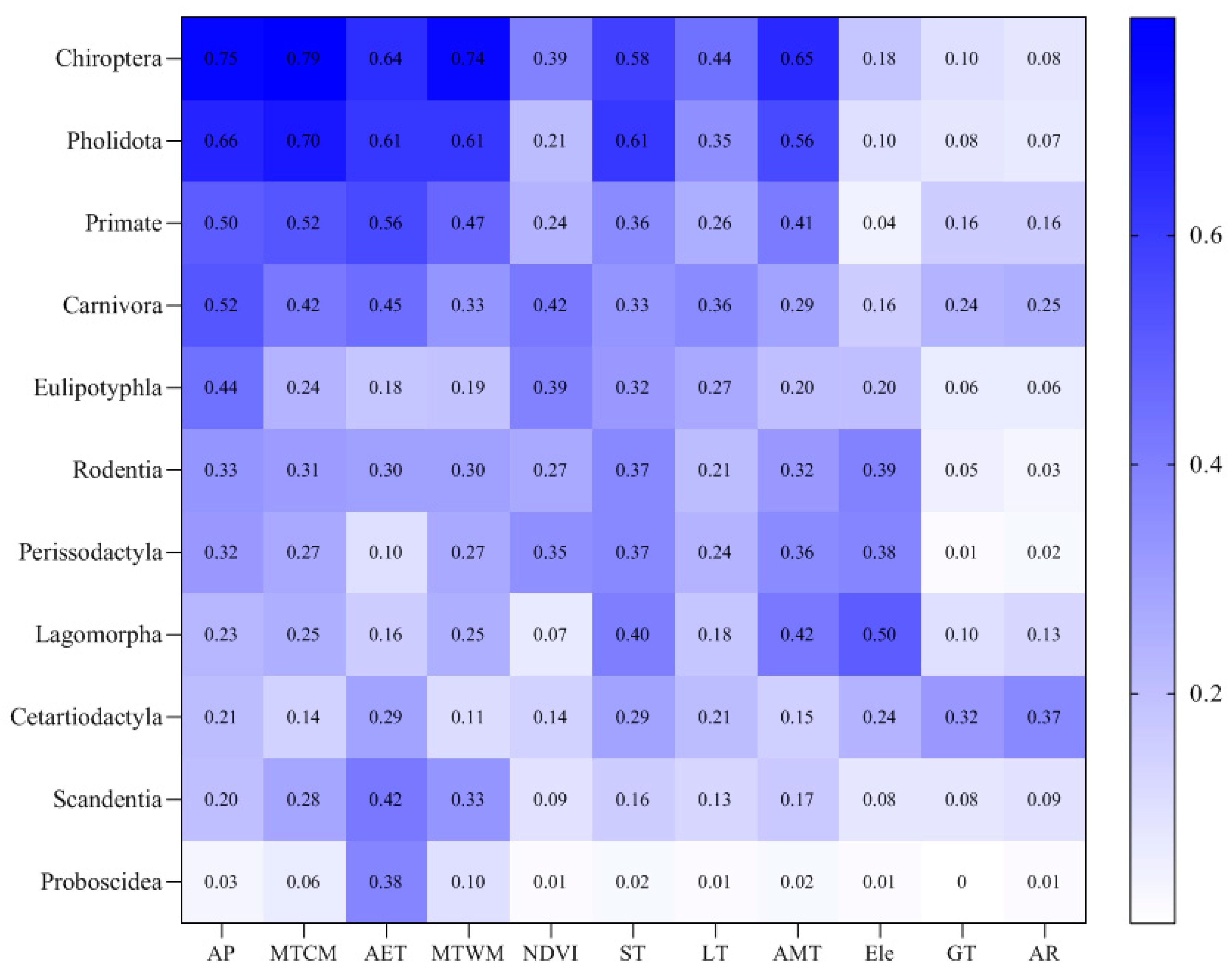
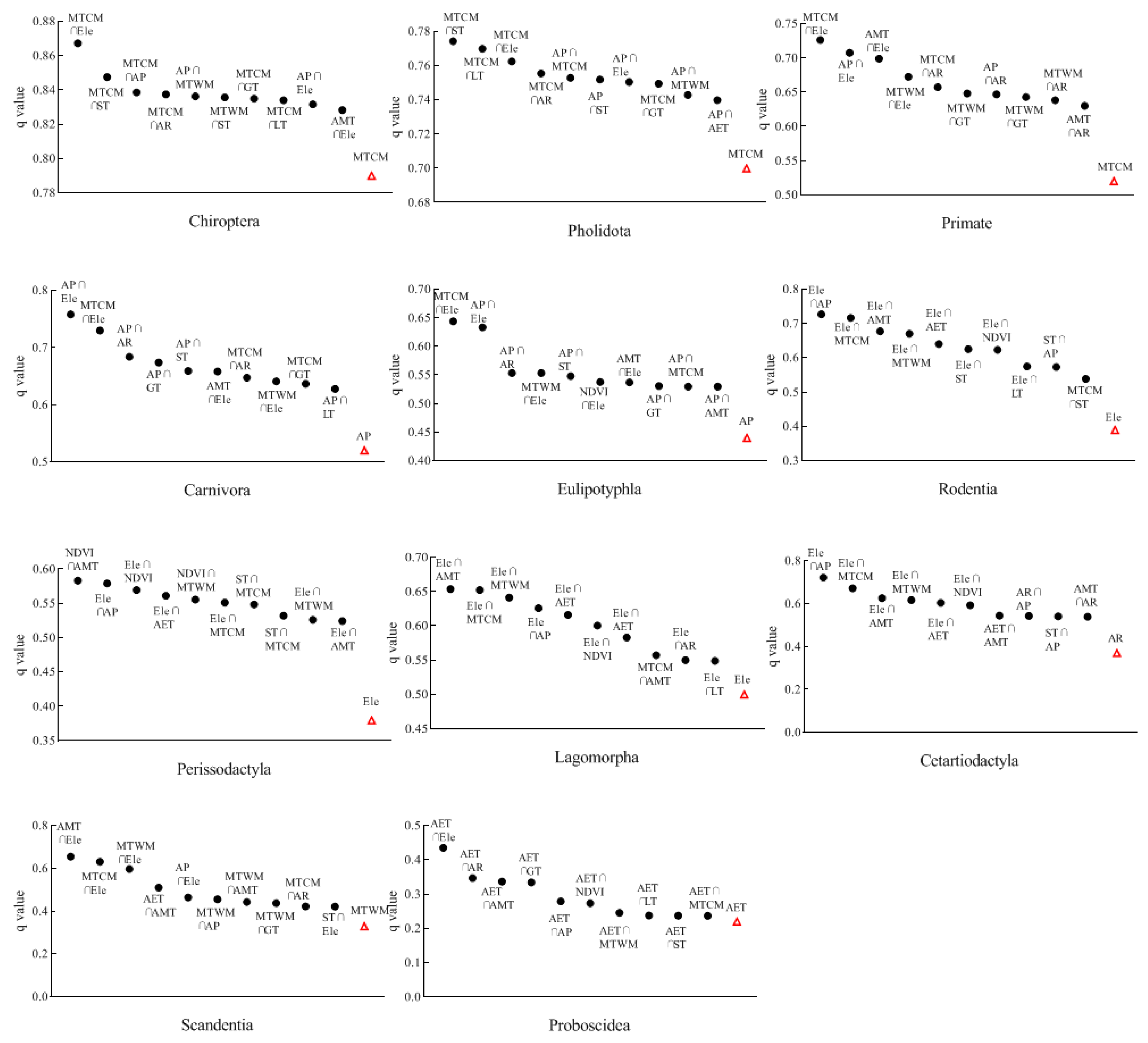
3.2. Influencing Factors on the Distribution of Mammalian Orders

We analyzed 11 orders of terrestrial mammals, and their distribution ranges are shown in Figure S1 (Supplementary Materials). The overall characteristics of orders were similar, with most of them showing lower species richness in the north and higher species richness in southwest China. We utilized the factor detector to determine the influence of environmental factors on different order richness.

The richness distribution of most orders was mainly affected by MTCM and AP. Chiroptera is mostly concentrated in southern China and low in most regions in the north. The geographical environment factors that mainly influenced the distribution of species richness of Chiroptera (Figure 4) were MTCM, AP, and MTWM. AR minimally affected distribution. The order of Pholidota has few species with a small distribution in China. The environmental factors affecting the richness distribution of Pholidota were similar to those of Chiroptera. The species in Primates are only distributed in southern China. The richness distribution of primates was significantly affected by MTCM and AP. Carnivora have a wide distribution of richness in China. AP and AET were the main factors affecting species richness distribution. Eulipotyphla are spread all over the country, except for the Qinghai–Tibetan Plateau. AP, with the largest q value, had a remarkable effect on the spatial distribution of species richness of Eulipotyphla, followed by NDVI.

The species richness of Rodentia, Perissodactyla, and Lagomorpha was affected by elevation, soil type, and AMT. Rodentia is widespread all over the country. The species distribution of Rodentia was affected by the elevation and soil type. Perissodactyla is only distributed in western China, strongly influenced by the elevation and ST. The species richness of Lagomorpha is highest in the eastern Qinghai–Tibetan Plateau. Elevation had a marked impact on the distribution of species richness of Lagomorpha. The q value of Ele was 0.50, followed 0.42 for AMT. However, the environmental factors influencing the species richness of Cetartiodactyla, Scandentia, and Proboscidea were different from other orders. Cetartiodactyla species richness in the north is lower than that in the south. Cetartiodactyla with differences in distribution richness was mainly related to AR and GT. The distribution range of Scandentia is too small, with species being significantly affected by AET. Proboscidea is distributed in a small area, not affected by any of the environmental variables except for AET.

We used the interaction detector to identify the interaction effect between environmental factors on the distribution of species richness of different orders. The interaction effects of pairs of environmental factors were nonlinear enhanced and bivariate enhanced. The results showed that the interaction relationships for the two factors enhanced the influence of species richness (Figure 5). The species richness distribution of Chiroptera was significantly influenced by MTCM, and the interaction between MTCM and other factors enhanced the influence effect. The influence of environmental factors on the distribution of Chiroptera and Pholidota was similar. MTCM was a significant single factor, while the influence of the interaction between MTCM and other factors was more significant on the species richness of Pholidota. The species richness distribution of Primates was more affected by MTCM and less affected by Ele. However, the interaction between Ele and any of MTCM, AP, and AMT had a more obvious impact on the species richness of Primates. AP was the main factor affecting the species distribution of Carnivora, and the interaction with other factors enhanced the effect. The influence of Ele on species richness of Carnivora was minimal, but the interaction of Ele with AP, MTCM, and AMT was more significant. The environmental factors affecting the richness distribution of Eulipotyphla were similar to Carnivora. AP was the main influencing factor, but the interaction of Ele with other factors had a more obvious influence on richness, especially the interaction between MTCM and Ele. The species distribution of Perissodactyla was significantly affected by Ele. The interaction of Ele with other factors enhanced the influence on species richness of Perissodactyla but was less than the combined effect of NDVI and AMT. The environmental factors influencing the richness distribution of Lagomorpha and Rodentia were similar. Ele was the main influence factor, and the interaction with other factors enhanced the influence. The distribution of species richness of Cetartiodactyla was significantly affected by AR, but the interaction of Ele and other factors strengthened the influence. The richness distribution of Scandentia was mainly affected by the single factor of MTWM. However, the Ele interaction with AMT, MTCM, and MTWM had a greater impact on richness distribution, followed by the MTWM interaction with other factors. The species richness of Proboscidea was most affected by AET. AET combined with other factors had a greater influence on the distribution of Proboscidea. GT and AR had little influence on species richness distribution of different orders, but the interaction with other factors could enhance the influence on species richness. The interaction between the two factors was greater than the influence of a single factor on species richness.

3.3. Indication of Environment Factors on the Distribution of Mammal Richness

Analysis of factor detector models allowed factors to be screened out that had significant effects on the distribution of animals among many environmental indicators. Each species has its unique range of habitats, with the risk detector allowing the appropriate types and ranges of mammalian species in environmental factors to be analyzed (confidence level 95%).

In areas where the annual precipitation was 897.83–1146.46 mm, species richness was the most abundant. However, below the level of 305.96–480.55 mm of the AP, less precipitation was not conducive to the aggregation of many species. For the terrestrial mammal richness, most of the species richness was in the AMT range of 20.28–28.23 °C (Figure 6). However, when the annual mean temperature was below zero, the species richness was low. The species richness was most abundant in the range 13.28–23.65 °C of MTWM and the range 6.39–17.64 °C of MTCM. Extremely low ambient temperatures had negative impacts on the distribution of animals. In areas where the actual evapotranspiration was large, the species richness was high. A higher vegetation index denoted a higher species richness. Mammalian species richness was the most abundant in forest land, with some mammals mainly distributed in shrub wood. However, the species richness was low on unused land, including bare areas, where land is difficult to be used. Terrestrial mammals were mainly distributed in areas with ferralsols. These soils were mainly distributed in humid tropical and subtropical regions. At the elevation range of 1905.60–2562.62 m, species richness was greatest but then decreased with increasing altitude. Species richness was abundant at 2613–3816 m of altitude relief, but richness declined when altitude relief was too flat. There was a high level of species richness in the extremely undulating mountains, and there were significant differences among the landform types.

4. Discussion

Our analysis showed that annual precipitation served as the most influential factor on the spatial distribution of mammalian richness in China. Of note, this view is also supported by Medellín, who suggested that annual precipitation is an essential cause of mammal richness [3]. Precipitation and vegetation are generally considered to have non-negligible influences on mammal distribution. Most animals in the world depend mainly on grassland vegetation as their source of food [47]. It is known that plant productivity is influenced by precipitation [48,49]. Changes in vegetation in turn affect the distribution and abundance of mammals [50]. Our findings are similar to those of Lin et al. [51], who identified that NDVI has an important influence on the spatial pattern of species richness of various groups according to the optimal linear model. The minimum temperature of the coldest month and the maximum temperature of the warmest month (MTWM) have a rather significant positive impact on mammal richness. Most mammals as endothermic vertebrates are dependent on productivity or the environmental climate, partly because of the mechanisms used to regulate temperature. For instance, as the ambient temperature changes, this group needs to consume a lot of energy to maintain a constant body temperature [52]. At present, much research has shown that MTCM is a remarkable factor affecting the distribution of animals [13,14]. Schap et al. [53] analyzed the relationships between Rodentia and Lagomorpha crown height and diversity with current climate conditions, finding strong correlations of community structure parameters with the maximum temperature of the warmest month and minimum temperature of the coldest month. We found that AET played an important role in the distribution of species richness. As revealed in Torres-Romero and Olalla-Tarraga [54], actual evapotranspiration is the key factor that affects the distribution of mammalian species richness worldwide.

Our result indicated that most mammalian orders were mainly affected by regional freezing tolerance and productivity levels (especially MTCM and AP). Topography, climate, vegetation, and other factors act together on mammals, resulting in different types of mammals adapting to various environments, in terms of morphological structure and living habits. The Chiroptera are not poikilothermic animals, divided into Megachiroptera and Microchiroptera. All species of Megachiroptera studied are homeothermic animals, with constant body temperatures regardless of the temperature of the surrounding environment to a large extent. Species of Microchiroptera on the other hand show different degrees of heterothermy [55]. In many species of Microchiroptera, body temperature and metabolic rate rise only during activity. This makes them homeothermic when they are active and poikilothermic when they are at rest [56]. Thus, the survival of Microchiroptera is closely related to the environment, especially temperature. Primates are widely distributed in tropical and subtropical regions, mostly inhabiting forests [57], and the extremely low temperature limits their activities. In reverse, Perissodactyla was mainly affected by habitat heterogeneity, and regional productivity levels had less impact on Lagomorpha. Perissodactyla includes mainly large-scale herbivores [58], which occur in the steppe, semi-desert, and desert environments. They inhabit mountainous areas or open areas of plateaus, which are strongly influenced by elevation and soil type. Most species of Lagomorpha occupy alpine habitats, mainly affected by elevation. The degree of influence was higher than the environmental heat factor. Most species of Eulipotyphla feed on insects and small animals, while others feed on plant rhizome and leaf fruits, which are closely associated with the vegetation index.

Analyses of the spatial distribution of animals have shifted from qualitative to quantitative by combining GIS spatial analysis with statistical methods. By taking advantage of GIS spatial data analysis, we used the latest data and measured the spatial distribution patterns of terrestrial mammals in China on 10 by 10 km geographic grids. Compared with previous studies limited to administrative districts or smaller areas, the area of the study unit eliminated the influence of area on species richness, controlled for single variables, and we compared other factors to animal distribution under the same conditions.

The main distinctions among methods involve the type of data they use. Ecological niche models perform well in predicting species potential distribution and provide response curves for each variable. However, most of them are based on the presence data of species. We aimed to quantitatively analyze the influence of geographical factors on the spatial distribution of terrestrial mammalian richness in China. However, there is no systematic collection of the presence–absence data of China’s mammals. In the study, mammal species distribution data were obtained from China’s Mammal Diversity and Geographic Distribution [39], which is more systematic, organized by many zoologists. At the same time, we selected categorical variables, including soil, landform, and land use as environmental factors. Geodetector analysis is based on a statistical relationship [59], which does not provide a spatial output. There are differences with ecological niche models. However, the Geodetector model is more conducive to the spatial stratification of different types of qualitative data. It can quantify the type of soil, landform, and land use to explain the stratification of mammalian distribution.

We aimed to present possibilities of using Geodetector to analyze the environmental factors that influence the distribution of species richness. Geodetector can identify appropriate types and ranges of the determinants of stratified heterogeneity of dependent variables more comprehensively. The factor detector in Geodetector reveals the relative importance or influence of variables related to the species richness without any assumptions or limitations compared to the traditional statistical methods. The ecological detector in Geodetector identifies the difference in impact between the two explanatory variables. The risk detector in Geodetector can screen out the range of geographical environments suitable for the survival of multiple animals. It provides a better comparison of species distribution with different stratifications of different environmental factors. Using the interaction detector in Geodetector to explore the interaction of two factors, a new perspective is provided in studies of mammalian distributions. The results show that two-factor interaction significantly enhances the influence of independent environmental factors on mammalian richness distribution.

The variable must be categorical in the Geodetector models. However, to comprehensively analyze the effects of environmental factors on mammalian species richness, we must select numerical variables and categorical variables. Numerical variables should be transformed to a category, which inevitably leads to information loss. A more detailed stratification of numerical environmental factors leads to less information loss and denote a more significant impact on the target factor. We divided the numerical variables into 10 categories, 20 categories, 30 categories, and 50 categories, and the q value of each numerical variable did not change much. The results show that, no matter how each numerical variable is classified, its influence on species richness is within a certain range. The relative influence of various numerical variables on species richness did not change. The soil type consisted of 13 soil orders, and the landform type and land-use type had eight categories. To keep small differences in categories between numerical variables and categorical variables, we classified the values of eight numerical variables into 10 classes. There are also other potential factors having major effects on mammalian richness. In subsequent analysis, more variables will be selected for a more detailed discrete classification to comprehensively evaluate the influence of environmental factors on the distribution of mammalian species richness. In conclusion, we discovered that Geodetector is an important and promising tool for ecologists to analyze and study species richness.

5. Conclusions

We evaluated the spatial distribution patterns of terrestrial mammal richness and analyzed the main factors influencing distribution differences in species richness. This research contributes to identifying spatial differences in mammalian richness, comprehensively considering climate, precipitation, topography, and vegetation factors, using the Geodetector model to discuss the influence strength and synergistic effect between key factors. The main conclusions are as follows:

(1)

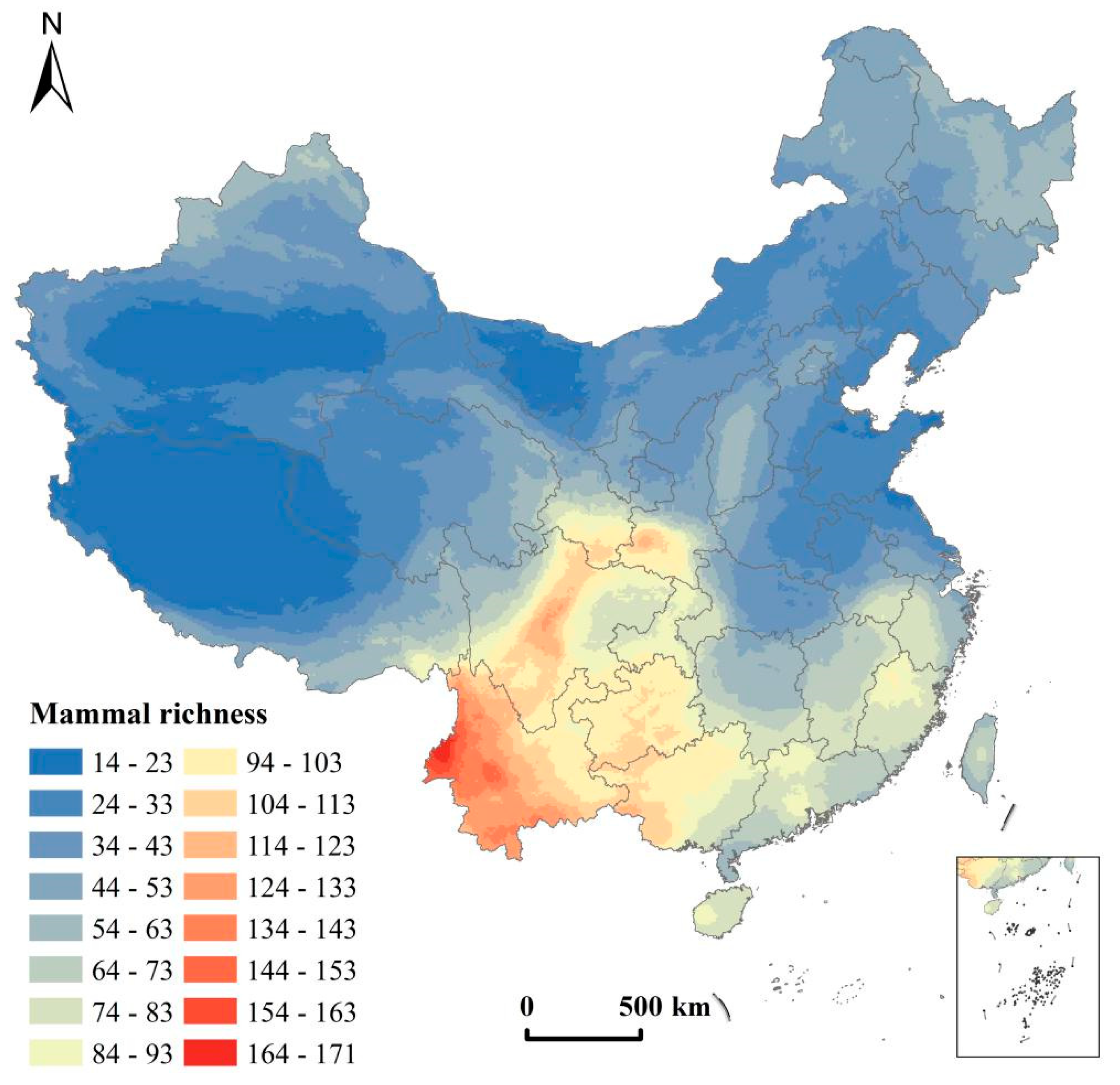
The spatial pattern of terrestrial mammals in China showed a low east–west trend and distinct heterogeneity to the north and south. AP and MTCM were the dominant factors affecting the spatial differentiation of mammal richness in China.

(2)

The characteristics of the distribution of species richness across taxonomic groups were influenced by different environmental factors. Many mammalian orders were affected by regional freezing tolerance and productivity levels (mainly MTCM and AP). Perissodactyla was mainly influenced by habitat heterogeneity, while regional productivity levels had less impact on Lagomorpha.

(3)

Extremely low ambient temperatures had negative impacts on the distribution of animals, with too little precipitation not being conducive to the aggregation of many species. At a certain altitude, mammalian taxonomic richness decreased with increasing altitude. Fewer mammals were present in regions where the altitude was too flat, with most mammals occurring in forest land.

(4)

The interactions of any two environmental factors had remarkable bivariate enhancement or nonlinear enhancement effects on the spatial distribution of species richness with respect to individual variables. The synergies of elevation with the minimum temperature of the coldest month and annual precipitation can best explain the regional distribution differences in mammal richness in China.

Our study provides a more accurate understanding of the extent to which species distributions are influenced by individual environmental factors and their pairs. We aim to facilitate the wider use of Geodetector by ecologists. Consequently, our findings can be used for the remote sensing monitoring of animal protection, which could help toward understanding the distribution range of terrestrial mammals and key control zones in protected areas from the macro perspective. It could also help give some reference evidence for the conservation policy of species diversity. Furthermore, some human activities such as overgrazing and deforestation might affect the distribution of animals by destroying existing habitats. The effects of human activities on the spatial distribution patterns of terrestrial mammals must be accounted for in future studies to mitigate the loss of biodiversity.

References

1. Scanes, C.G. Chapter 19—Human Activity and Habitat Loss: Destruction, Fragmentation, and Degradation. In Animals and Human Society; Scanes, C.G., Toukhsati, S.R., Eds.; Academic Press: Cambridge, MA, USA, 2018; pp. 451–482. [Google Scholar] [CrossRef]
2. Danell, K.; Lundberg, P.; Niemela, P. Species richness in mammalian herbivores: Patterns in the boreal zone. Ecography 1996, 19, 404–409. [Google Scholar] [CrossRef]
3. Medellín, R.A. Mammal diversity and conservation in the selva-lacandona, Chiapas, Mexico. Conserv. Biol. 1994, 8, 780–799. [Google Scholar] [CrossRef]
4. Andrews, P.; O’Brien, E.M. Climate, vegetation, and predictable gradients in mammal species richness in southern Africa. J. Zool. 2000, 251, 205–231. [Google Scholar] [CrossRef]
5. Badgley, C.; Fox, D.L. Ecological biogeography of North American mammals: Species density and ecological structure in relation to environmental gradients. J. Biogeogr. 2000, 27, 1437–1467. [Google Scholar] [CrossRef] [Green Version]
6. Brown, J.H. Two decades of homage to santa-rosalia—Toward a general-theory of diversity. Am. Zool. 1981, 21, 877–888. [Google Scholar] [CrossRef] [Green Version]
7. Wright, D.H. Species-energy theory—An extension of species-area theory. Oikos 1983, 41, 496–506. [Google Scholar] [CrossRef] [Green Version]
8. Turner, J.R.G.; Lennon, J.J.; Lawrenson, J.A. British bird species distributions and the energy theory. Nature 1988, 335, 539–541. [Google Scholar] [CrossRef]
9. Currie, D.J. Energy and large-scale patterns of animal-species and plant-species richness. Am. Nat. 1991, 137, 27–49. [Google Scholar] [CrossRef]
10. Connell, J.H.; Orias, E. The ecological regulation of species diversity. Am. Nat. 1964, 98, 399–414. [Google Scholar] [CrossRef]
11. Stevens, G.C. The latitudinal gradient in geographical range—How so many species coexist in the tropics. Am. Nat. 1989, 133, 240–256. [Google Scholar] [CrossRef]
12. O’Brien, E.M. Climatic gradients in woody plant-species richness—Towards an explanation-based on an analysis of Southern Africa woody flora. J. Biogeogr. 1993, 20, 181–198. [Google Scholar] [CrossRef]
13. Hawkins, B.A.; Porter, E.E.; Diniz, J.A.F. Productivity and history as predictors of the latitudinal diversity gradient of terrestrial birds. Ecology 2003, 84, 1608–1623. [Google Scholar] [CrossRef] [Green Version]
14. Hawkins, B.A. Ecology’s oldest pattern? Trends Ecol. Evol. 2001, 16, 470. [Google Scholar] [CrossRef]
15. Kerr, J.T.; Packer, L. Habitat heterogeneity as a determinant of mammal species richness in high-energy regions. Nature 1997, 385, 252–254. [Google Scholar] [CrossRef]
16. Ricklefs, R.E. Community diversity—Relative roles of local and regional processes. Science 1987, 235, 167–171. [Google Scholar] [CrossRef] [PubMed]
17. Maldonado, A.D.; Ropero, R.F.; Aguilera, P.A.; Rumi, R.; Salmeron, A. Continuous Bayesian networks for the estimation of species richness. Prog. Artif. Intell. 2015, 4, 49–57. [Google Scholar] [CrossRef]
18. Grenyer, R.; Orme, C.D.L.; Jackson, S.F.; Thomas, G.H.; Davies, R.G.; Davies, T.J.; Jones, K.E.; Olson, V.A.; Ridgely, R.S.; Rasmussen, P.C.; et al. Global distribution and conservation of rare and threatened vertebrates. Nature 2006, 444, 93–96. [Google Scholar] [CrossRef]
19. Huntley, B.; Berry, P.M.; Cramer, W.; McDonald, A.P. Modelling present and potential future ranges of some European higher plants using climate response surfaces. J. Biogeogr. 1995, 22, 967–1001. [Google Scholar] [CrossRef] [Green Version]
20. Vayssières, M.P.; Plant, R.E.; Allen-Diaz, B.H. Classification trees: An alternative non-parametric approach for predicting species distributions. J. Veg. Sci. 2000, 11, 679–694. [Google Scholar] [CrossRef]
21. De’ath, G. Multivariate regression trees: A new technique for modeling species—Environment relationships. Ecology 2002, 83, 1105–1117. [Google Scholar] [CrossRef]
22. Ostmann, A.; Arbizu, P.M. Predictive models using randomForest regression for distribution patterns of meiofauna in Icelandic waters. Mar. Biodivers. 2018, 48, 719–735. [Google Scholar] [CrossRef]
23. Elith, J.; Leathwick, J.R.; Hastie, T. A working guide to boosted regression trees. J. Anim. Ecol. 2008, 77, 802–813. [Google Scholar] [CrossRef] [PubMed]
24. Sillero, N.; Barbosa, A.M. Common mistakes in ecological niche models. Int. J. Geogr. Inf. Sci. 2020, 1–14. [Google Scholar] [CrossRef]
25. Aguilar, M.; Lado, C. Ecological niche models reveal the importance of climate variability for the biogeography of protosteloid amoebae. ISME J. 2012, 6, 1506–1514. [Google Scholar] [CrossRef] [PubMed] [Green Version]
26. Wang, J.F.; Xu, C.D. Geodetector: Principle and prospective. Acta Geogr. Sin. 2017, 72, 116–134. [Google Scholar] [CrossRef]
27. Wang, J.F.; Zhang, T.L.; Fu, B.J. A measure of spatial stratified heterogeneity. Ecol. Indic. 2016, 67, 250–256. [Google Scholar] [CrossRef]
28. Wang, J.F.; Li, X.H.; Christakos, G.; Liao, Y.-L.; Zhang, T.; Gu, X.; Zheng, X.-Y. Geographical Detectors-Based Health Risk Assessment and its Application in the Neural Tube Defects Study of the Heshun Region, China. Int. J. Geogr. Inf. Sci. 2010, 24, 107–127. [Google Scholar] [CrossRef]
29. Chen, C.L.; Zhang, Q.J.; Lv, X.; Huang, X.J. Analysis on spatial-temporal characteristics and driving mechanisms of cropland occupation and supplement in Jiangsu Province. Econ. Geogr. 2016, 36, 155–163. [Google Scholar]
30. Zou, B.; Xu, S.; Zhang, J. Spatial Variation Analysis of Urban Air Pollution Using GIS: A Land Use Perspective. Geomat. Inf. Sci. Wuhan Univ. 2017, 42, 216–222. [Google Scholar]
31. Shen, J.; Zhang, N.; He, B.; Liu, C.Y.; Li, Y.; Zhang, H.Y.; Chen, X.Y.; Lin, H. Construction of a GeogDetector-based model system to indicate the potential occurrence of grasshoppers in Inner Mongolia steppe habitats. Bull. Entomol. Res. 2015, 105, 335–346. [Google Scholar] [CrossRef] [Green Version]
32. Fan, L.X.; Wu, E.Q.; Liu, J.; Qu, X.C.; Liu, C.; Ning, B.A.; Liu, Y. Distribution Characteristics of Spermophilus dauricus in Manchuria City in China in 2015 through ‘3S’ Technology. Biomed. Environ. Sci. 2016, 29, 603–608. [Google Scholar] [CrossRef] [PubMed]
33. Chen, G.; Wang, W.; Liu, Y.; Zhang, Y.; Ma, W.; Xin, K.; Wang, M. Uncovering the relative influences of space and environment in shaping the biogeographic patterns of mangrove mollusk diversity. ICES J. Mar. Sci. 2019, 1–10. [Google Scholar] [CrossRef]
34. Liu, T.; Wang, J.; Xu, C.; Ma, J.; Zhang, H.; Xu, C. Sandwich mapping of rodent density in Jilin Province, China. J. Geogr. Sci. 2018, 28, 445–458. [Google Scholar] [CrossRef] [Green Version]
35. Liu, B.; Jiao, Z.; Ma, J.; Gao, X.; Xiao, J.; Muhammad Abid Hayat, W.H. Modelling the potential distribution of arbovirus vector Aedes aegypti under current and future climate scenarios in Taiwan, China. Pest. Manag. Sci. 2019, 75, 3076–3083. [Google Scholar] [CrossRef] [PubMed]
36. Liu, B.; Gao, X.; Zheng, K.; Ma, J.; Jiao, Z.; Xiao, J.; Wang, H. The potential distribution and dynamics of important vectors Culex pipiens pallens and Culex pipiens quinquefasciatus in China under climate change scenarios: An ecological niche modelling approach. Pest. Manag. Sci. 2020, 76, 3096–3107. [Google Scholar] [CrossRef]
37. Watson, J.E.M.; Rao, M.; Kang, A.L.; Xie, Y. Climate change adaptation planning for biodiversity conservation: A review. Adv. Clim. Chang. Res. 2012, 3, 1–11. [Google Scholar] [CrossRef]
38. Zhang, R. Geological events and mammalian distribution in China. Acta Zool. Sin. 2002, 48, 141–153. [Google Scholar]
39. Jiang, Z.; Ma, Y.; Wu, Y.; Wang, Y.; Zhou, K.; Liu, S.; Feng, Z. China’s Mammal Diversity and Geographical Distribution; China Science Publishing: Beijing, China, 2015. [Google Scholar]
40. Turner, J.R.G.; Gatehouse, C.M.; Corey, C.A. Does solar-energy control organic diversity—Butterflies, moths and the British climate. Oikos 1987, 48, 195–205. [Google Scholar] [CrossRef]
41. Abramsky, Z.; Rosenzweig, M.L. Tilman predicted productivity diversity relationship shown by desert rodents. Nature 1984, 309, 150–151. [Google Scholar] [CrossRef]
42. Currie, D.J.; Paquin, V. Large-scale biogeographical patterns of species richness of trees. Nature 1987, 329, 326–327. [Google Scholar] [CrossRef]
43. Tews, J.; Brose, U.; Grimm, V.; Tielborger, K.; Wichmann, M.C.; Schwager, M.; Jeltsch, F. Animal species diversity driven by habitat heterogeneity/diversity: The importance of keystone structures. J. Biogeogr. 2004, 31, 79–92. [Google Scholar] [CrossRef] [Green Version]
44. Jenks, G.F. The data model concept in statistical mapping. Int. Yearb. Cartogr. 1967, 7, 186–190. [Google Scholar]
45. Ding, Y.T.; Zhang, M.; Qian, X.Y.; Li, C.R.; Chen, S.; Wang, W.W. Using the geographical detector technique to explore the impact of socioeconomic factors on PM2.5 concentrations in China. J. Clean. Prod. 2019, 211, 1480–1490. [Google Scholar] [CrossRef]
46. Zhu, L.; Meng, J.; Zhu, L. Applying Geodetector to disentangle the contributions of natural and anthropogenic factors to NDVI variations in the middle reaches of the Heihe River Basin. Ecol. Indic. 2020, 117, 106545. [Google Scholar] [CrossRef]
47. Eronen, J.T.; Puolamaki, K.; Liu, L.; Lintulaakso, K.; Damuth, J.; Janis, C.; Fortelius, M. Precipitation and large herbivorous mammals I: Estimates from present-day communities. Evol. Ecol. Res. 2010, 12, 217–233. [Google Scholar]
48. Reich, P.B.; Walters, M.B.; Ellsworth, D.S. From tropics to tundra: Global convergence in plant functioning. Proc. Natl. Acad. Sci. USA 1997, 94, 13730–13734. [Google Scholar] [CrossRef] [Green Version]
49. Walker, B.H.; Langridge, J.L. Predicting savanna vegetation structure on the basis of plant available moisture (PAM) and plant available nutrients (PAN): A case study from Australia. J. Biogeogr. 1997, 24, 813–825. [Google Scholar] [CrossRef]
50. Witecha, M.J. Effects of Fire and Precipitation on Small Mammal Populations and Communities; Texas A&M University: Kingsville, TX, USA, 2011. [Google Scholar]
51. Lin, X.; Wang, Z.; Tang, Z.; Zhao, S.; Fang, J. Geographic patterns and environmental correlates of terrestrial mammal species richness in China. Biodivers. Sci. 2009, 17, 652–663. [Google Scholar]
52. Wang, Z.; Tang, Z.; Fan, J. The species-energy hypothesis as a mechanism for species richness patterns. Biodivers. Sci. 2009, 17, 613–624. [Google Scholar]
53. Schap, J.A.; Samuels, J.X.; Joyner, T.A. Ecometric estimation of present and past climate of North America using crown heights of rodents and lagomorphs. Palaeogeogr. Palaeoclimatol. Palaeoecol. 2020. [Google Scholar] [CrossRef]
54. Torres-Romero, E.J.; Olalla-Tarraga, M.A. Untangling human and environmental effects on geographical gradients of mammal species richness: A global and regional evaluation. J. Anim. Ecol. 2015, 84, 851–860. [Google Scholar] [CrossRef] [PubMed] [Green Version]
55. Kulzer, E. Temperaturregulation bei Fledermäusen (Chiroptera) aus verschiedenen Klimazonen. Z. Vgl. Physiol. 1965, 50, 1–34. [Google Scholar] [CrossRef]
56. Reeder, W.G.; Cowles, R.B. Aspects of Thermoregulation in Bats. J. Mammal. 1951, 32, 389–403. [Google Scholar] [CrossRef]
57. Martin, R.D. Primates, Evolution of. In International Encyclopedia of the Social & Behavioral Sciences; Smelser, N.J., Baltes, P.B., Eds.; Pergamon: Oxford, UK, 2001; pp. 12032–12038. [Google Scholar] [CrossRef]
58. Berkovitz, B.; Shellis, P. Chapter 12—Perissodactyla. In The Teeth of Mammalian Vertebrates; Berkovitz, B., Shellis, P., Eds.; Academic Press: Cambridge, MA, USA, 2018; pp. 213–221. [Google Scholar] [CrossRef]
59. He, J.; Pan, Z.; Liu, D.; Guo, X. Exploring the regional differences of ecosystem health and its driving factors in China. Sci. Total Environ. 2019, 673, 553–564. [Google Scholar] [CrossRef] [PubMed]
Figure 1. Topography of China.
Ijgi 10 00021 g001
Figure 2. Distribution of environmental factors in the study area.
Ijgi 10 00021 g002aIjgi 10 00021 g002bIjgi 10 00021 g002c
Figure 3. Distribution pattern of terrestrial mammal richness in China.
Ijgi 10 00021 g003
Figure 4. Influence of environmental factors on the richness distribution of mammalian orders (q values).
Ijgi 10 00021 g004
Figure 5. Interaction factors and single factors mainly affecting the species richness of each order.
Ijgi 10 00021 g005
Figure 6. The appropriate range of environmental factors for the richness distribution of terrestrial mammals.
Ijgi 10 00021 g006