Article

Sensitivity Assessment of Spatial Resolution Difference in DEM for Soil Erosion Estimation Based on UAV Observations: An Experiment on Agriculture Terraces in the Middle Hill of Nepal

1
Central Department of Geography, Tribhuvan University, Kirtipur 44618, Nepal
2
Branch of Sustainable Mountain Development, Kathmandu Center for Research and Education, Chinese Academy of Sciences-Tribhuvan University, Chengdu 610041, China
3
Institute of Mountain Hazards and Environment, Chinese Academy of Sciences, Chengdu 610041, China
*
Author to whom correspondence should be addressed.
ISPRS Int. J. Geo-Inf. 2021, 10(1), 28; https://0-doi-org.brum.beds.ac.uk/10.3390/ijgi10010028
Submission received: 3 December 2020 / Revised: 6 January 2021 / Accepted: 11 January 2021 / Published: 13 January 2021
(This article belongs to the Special Issue Geomorphometry and Terrain Analysis)

Abstract

:
Soil erosion in the agricultural area of a hill slope is a fundamental issue for crop productivity and environmental sustainability. Building terrace is a very popular way to control soil erosion, and accurate assessment of the soil erosion rate is important for sustainable agriculture and environmental management. Currently, many soil erosion estimations are mainly based on the freely available medium or coarse resolution digital elevation model (DEM) data that neglect micro topographic modification of the agriculture terraces. The development of unmanned aerial vehicle (UAV) technology enables the development of high-resolution (centimeter level) DEM to present accurate topographic features. To demonstrate the sensitivity of soil erosion estimates to DEM resolution at this high-resolution level, this study tries to evaluate soil erosion estimation in the Middle Hill agriculture terraces in Nepal based on UAV derived high-resolution (5 × 5 cm) DEM data and make a comparative study for the estimates by using the DEM data aggregated into different spatial resolutions (5 × 5 cm to 10 × 10 m). Firstly, slope gradient, slope length, and topographic factors were calculated at different resolutions. Then, the revised universal soil loss estimation (RUSLE) model was applied to estimate soil erosion rates with the derived LS factor at different resolutions. The results indicated that there was higher change rate in slope gradient, slope length, LS factor, and soil erosion rate when using DEM data with resolution from 5 × 5 cm to 2 × 2 m than using coarser DEM data. A power trend line was effectively used to present the relationship between soil erosion rate and DEM resolution. The findings indicated that soil erosion estimates are highly sensitive to DEM resolution (from 5 × 5 cm to 2 × 2 m), and the changes become relatively stable from 2 × 2 m. The use of DEM data with pixel size larger than 2 × 2 m cannot detect the micro topography. With the insights about the influencing mechanism of DEM resolution on soil erosion estimates, this study provides important suggestions for appropriate DEM data selection that should be investigated first for accurate soil erosion estimation.

1. Introduction

Land is one of the most important natural resources for agricultural activities to support people’s livelihood [1]. As being a crucial issue of decreasing productivity, the loss of fertile soil induced by soil erosion frequently happens in hilly slopes [2], and the effects of soil erosion go beyond the loss of fertile land [3]. The global soil erosion rate was estimated at 35.9 Pg yr−1 in 2012, and there is a potentially increasing trend in global soil erosion driven by cropland expansion [4]. Under the background of climate change, soil erosion has been and will always be a key issue for the sustainable development at the framework of future earth [3,5]. Meanwhile, the catastrophic floods that have frequently happened in recent years greatly induced big amount of soil erosion, posing a big pressure on local agricultural development [6,7].
Usually, soil erosion process by water in the hill slope is highly controlled by its terrain features [8]. Therefore, increasing soil water retention capacity by improving infiltration and reducing peak discharge rate of surface runoff has been well recognized as the main direction for soil and water conservation. Terracing cultivated land in the hill slope can obviously achieved this effect [9]. Therefore, terrace is one of the most predominant forms of agriculture in the Asia and the Pacific regions [10].
As a typical mountain country in the South Asia, Nepal has experienced serious degradation of soil resources over the past three decades especially in the Middle Hills as a result of the expansion of agricultural land and the increase in cropping intensity [2]. The national land degradation assessment report has revealed that 3.16 million hectares (11.81% of the total area of Nepal) have been affected by the degradation process. To preserve soil and water resources, both irrigated contour terraces and rain-fed outward sloping terraces are found in most of the hill slopes of Nepal. The modification of topographic features at small scales by these terraces greatly controls soil erosion [11], which is a long tradition of soil erosion controlling technique in the cultivated hill slope of Nepal. Farmers maintain their agriculture terraces regularly. They also grow trees at rain-fed agriculture terraces to stabilize it and fodder supply for their livestock [12]. These are the major characteristics of integrated subsistence farming system of agriculture hill slopes of Nepal.
From field measurements, it has been confirmed that the controlling effect of soil erosion is quite different for different types of terraces [13]. Thus, accurate detection of real topographic features of hilly slopes is crucial for soil erosion monitoring and regulation in the slope. With the development of digital elevation model (DEM), data are a powerful vehicle for conveying essential surface topographic information, which is very useful for terrain analysis of physical surface including various hydrological and biophysical properties [14]. Therefore, the resolution of the DEM data plays an important role in controlling the soil erosion assessment. Currently, many models have been designed for soil erosion estimation, such as the universal soil loss equation (USLE), modified universal soil loss equation (MUSLE), and revised universal soil loss equation (RUSLE). The RUSLE model estimates sheet and rill erosion caused by raindrop impact [15], and this model does not cover the gully erosion. With the combination of geographic information system (GIS) and remote sensing technologies, RUSLE estimates soil erosion loss on a cell-by-cell basis. Soil and water assessment that uses DEMs with the resolutions from 5 × 5 to 14 × 14 m reveals the decreasing trend when DEMs were resampled to coarser [16]. Similar results were achieved by different studies with higher accuracies of higher resolution DEM as compared to coarse resolution [17,18]. Thus, there are the significant effects of spatial resolution of DEM on topography-based geomorphological and hydrological assessment [19,20,21,22,23].
From current studies, it can be concluded that most of them were conducted using the existing open-source DEMs, which range from 10 × 10 m to kilometer level. There is a lack of related discussions or analyses for high spatial resolution (sub-meter level) due to the limitations of such high-resolution DEM data. In recent years, the development of unmanned aerial vehicle (UAV) technique provides an easy tool to derive high resolution DEM with the spatial resolution of centimeter level [24]. Thus, the UAV-based high spatial resolution DEM offers valuable information of surface topography especially land surface processes and hydrological analysis. UAV-acquired high-resolution DEM has been popular for several geomorphological and hydrological analyses in recent decades [25,26,27], because it provides an important opportunity to estimate soil erosion at this high-resolution level. Therefore, with a view to accurate estimation of the soil erosion in Nepal, this study has been conducted to investigate the sensitivity of the estimated of soil erosion rates based on the RUSLE model for agriculture terraces in the hill slopes of Nepal. The findings of the study will be helpful to understand how far the spatial resolution of DEM is sensitive for the estimation of soil erosion rates and the values of topographic factors for geomorphic and hydrologic processes research, especially in the narrow agriculture terraces in the hill slopes such as those in Nepal.

2. Materials and Methods
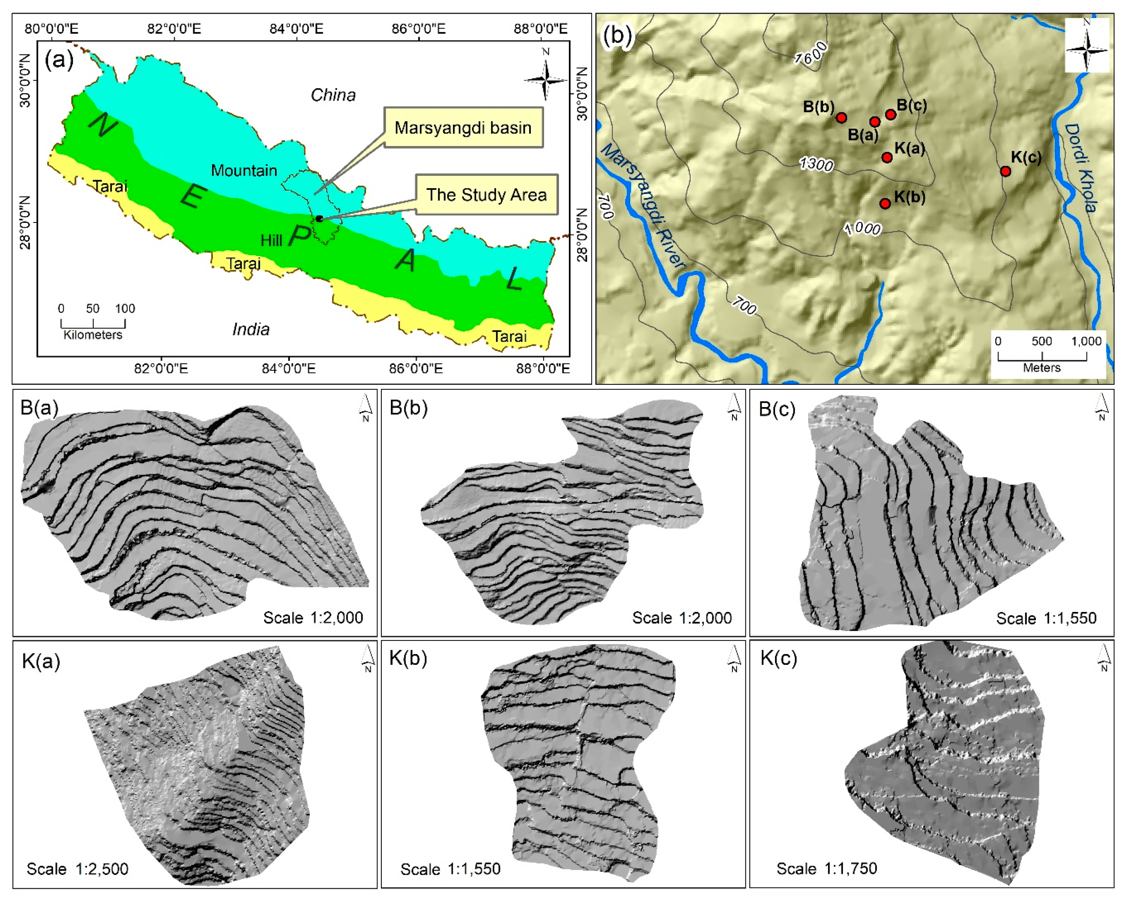
2.1. Study Area

The study area is located in the Marshynangdi river basin that lies in the hilly region of the central part of Nepal. The extension of the study area is 28°12′33″ north to 28°13′07″ north of latitude and 84°25′28″ east to 84°26′37″ east of longitude (Figure 1) with the elevation range from 1072 to 1593 m from the mean sea level. It has a warm temperate climate with an annual average rainfall of 3374 mm (more than 80% fall in summer season from May to August). Therefore, the summer season usually experiences the most serious soil erosion in this region.
Farmers manage their cultivated land by making complete horizontal terraces at irrigated plots and outward sloping terraces for rain-fed plots. They grow grasses and fodder trees at terrace riser. Intensive subsistence farming practice is evident in the area as intensive use of cultivated land, which integrates livestock, forest, and grasses in their system of livelihood. As shown in Figure 1, six plots were selected as the study areas. Among them, three were rain-fed and three were irrigated agriculture plots. In local term, a rain-fed cultivated terrace is known as bari, and an irrigated terrace is known as khet. Therefore, the selected rain-fed plots were named B(a), B(b), and B(c) plots, and the irrigated plots were named K(a), K(b), and K(c) plots. The total area of the selected plots was 3.22 hectares. The area of the smallest plot was 0.26 hectares, and the largest one was 1.23 hectares. The total area of the rain-fed plots was 1.39 hectares with the average size of 0.46 hectares. The total area of irrigated plots was 1.83 hectares with the average size of 0.61 hectares. The average slope gradient of the study plots is 18° ranging from 12 to 22°. In general, terrace sizes were bigger even in the steeper slopes of rain-fed terrace as compared to less steep slope K(a). Plots K(b) and K(c) were bigger terrace size due to the lower slope gradient as compared to other plots.

2.2. UAV-Based DEM Derivation

The UAV combined with a digital camera system allows for the acquisition of usable DEM data for geomatic application such as 3D mapping and modelling [28]. In this study, the DEM data of the study area were acquired in August 2018 during the period of off farming. In this period, the irrigated fields were opened after harvesting paddy and the rain-fed cultivated lands were opened after harvesting maize and the field preparation for millet plantation begins. It avoids the disturbances of crop plants to derive high-resolution images. Photogrammetry works on the basis of two or more overlapping (stereo pair) photographs to derive the unique three-dimensional location of a set of homogeneous image points of overlapping photographs, by which the position and orientation of the camera can be computed and can be obtained a mosaic orthoimage at the end [29,30]. The first requirement is the preparation for the scaling and georeferencing for the target surface to extract oriented and scaled data. At least three or more ground control points (GCP) are required for scaling and georeferencing [31]. Altogether, 57 GCP points were fixed in six plots, and the coordinates of these GCPs were measured with total station to enable their high accuracy. GCPs were easily distinguishable from the background, which was easily marked during the processing of aerial images. The coordinates of the GCPs were used as a reference location for photogrammetric processing of the aerial images and accuracy assessment of DEM [32,33,34].
The DJI Phantom 4 Pro Plus Quadcopter Drone with Deluxe Controller—CP.PT.000549 was used mounting GO PRO camera to capture low height remote sensing imagery [35]. The flight path was defined in the UAV control software. The flight route was designed in wind direction by which flying against the wind very slowly above ground speed could be achieved. It helps to avoid motion blur because of the conventional high-flying speed. When it was flying at the low altitude, it was not possible to capture the whole area with a 60% overlap in one flight due to the low trigger frequency of the camera. The flying speed was reduced as much as possible and multiple flights at the same flight altitude were done to acquire complete dataset to compensate the gaps. The flying height was from 50 to 100 m.
Agisoft Photoscan software was used for photogrammetric process [32,36]. Feature detection algorithm was applied to align overlapping images at first. The second step was to remove inconsistencies. The third one was to apply bundle adjustment algorithm to simultaneously solve the 3D geometry of the scenes [37]. The outputs of these steps were a sparse point cloud. The GCPs on the images were identified manually, and their coordinates were imported, which were used to refine the camera calibration parameters and to optimize the geometry of the output point cloud. The GCPs coordinates were used to refine the camera calibration parameters and optimize the geometry of the output point cloud. Multi-view stereo matching algorithm was used to increase the density of sparse point cloud, which is strongly related to the number of matching key points. A polygon mesh was created from the dense point cloud and a texture map derived from all images was applied to the polygon mesh and used to create an orthophoto. Then, DEM data with pixel size of 5 × 5 cm were generated.
The DEM accuracies were evaluated through the GCP coordinates. The root mean square error (RMSE) ranged from approximately 11 to 17 cm of X, 13 to 18 cm of Y, and 3 to 5 cm of Z [38]. The mean re-projection error was evaluated from 0.5 to 1.2 pixels. Based on the evaluated DEM data, seven other DEM data with different pixel sizes (10 × 10 cm, 20 × 20 cm, 50 × 50 cm, 1 × 1 m, 2 × 2 m, 5 × 5, and 10 × 10 m) were generated via spatial aggregation. The aggregation was done with order of 5 × 5 to 10 × 10 cm, 10 × 10 to 20 × 20 cm, 10 × 10 to 50 × 50 cm, 50 × 50 cm to 1 × 1 m, 1 × 1 to 2 × 2 m, 1 × 1 to 5 × 5 m, and 5 × 5 to 10 × 10 m. During the aggregation process, the mean values of the first level DEM data were transferred to the aggregated level according to previous geomorphological and hydrological analysis [39,40].

2.3. Soil Erosion Estimation Method

The widely used RUSLE was selected here to estimate soil erosion over the study area. This model is internationally applicable and provides comparatively reliable result [41,42,43,44]. This model is the most popular and reliable soil erosion model, which has been used around the world to predict long term rate of soil erosion from different farm size units subject to different management practices [45]. The structure of the RUSLE model can be expressed with the following equation. The average annual soil erosion rate is expressed in ton/hectare/year (t/h/y):
E = R*K*LS*C*P,
where,
E = Annual average soil erosion rate.
R = Rainfall erosivity.
K = Soil erodibility.
LS = Topographic factors.
C = Land cover management factor.
P = Protection factor.
According to this equation, it is known that the LS factor is the only factor that is highly connected with the surface topographic condition. For a certain plot, other factors can be thought to be invariant. Therefore, the impact from the DEM resolution can be directly assessed by calculating the LS factor with the eight DEM data. Detail processes in order to derive different factors are described.

2.3.1. LS Factor

The LS factor is the combined calculated values using slope gradient (s) and slope length (l). Slope gradient (s) is the steepness of slope, which has a positive impact on soil erosion rate; the slope length (l) is the distance from the point of origin of overland flow to the point where either the slope decreases to the extent that deposition begins or runoff water enters a well-defined channel. The soil erosion rate increases with the increase in slope length (l), but it has weaker strength to increase soil erosion rate with increasing slope length as compare to slope steepness (s) [45]. Topographic factors such as slope length (l), slope gradient (s), and LS factors were calculated using individual spatial resolution DEM for individual sampled plots. The following equations were used to derive slope length (l) and LS factors from DEM [46].
L S =   l 22 ( 0.065 + 0.045 s + 0.0065 s 2 )
where s is slope gradient, and it is used in percent slope. l is the slope length in meters, which is calculated using Equation (3)
l = 1.4 ( A s 22.13 ) 0.4
A s is unit contributing area (m²) [47].

2.3.2. R Factor

The local level climatic data are available for a very short period of time and meteorological stations are located at distant places. It is impossible to develop reliable high spatial resolution R factor data based on long term rainfall condition in the study area. Thus, rainfall erosivity (R factor) was collected from the European Soil Data Centre (ESDAC) at 1 km scale. It was calculated from the rainfall data of temporal coverage of 30–40 years with the unit of MJ mm/ha/h/y. These data were produced in 2013–2017 in collaboration between the European Commission (Joint Research Centre), the University of Basel, and the Meteorological and Environmental Institute [11]. The values of the R factor of each plot were determined according to the geolocation with the ESDAC product, with the range from 7331.9 to 9078.43 MJ mm/ha/h/y. The average value of R factor of the rain-fed plots was lower (7830.5 MJ mm/ha/h/y) than that of the irrigated plots (8528.4 MJ mm/ha/h/y). Plot K(c) has the highest value, while plot B(b) has the lowest value.

2.3.3. K Factor

Three soil samples from each selected plot were collected. Soil structures were identified from the field and other properties of the soil were derived by physical and chemical analysis in the laboratory. Soil erodibility factor (K) is the rate of soil loss per unit of R, as measured on a unit plot under specific condition. The soil erodibility factor (K) was calculated using the following equation:
K = 0.1317 * [ { 2.1 * 10 4 * M 1.14 * ( 12 a ) + 3.25 * ( b 2 ) + 2.5 * ( c 3 ) } / 100 ] ,
where
K is soil erodibility (t ha h/ha/MJ/mm).
M is soil textural factor (% silt + % very fine sand) × (100 − % clay).
a is organic matter content in percent (%) in the soil.
b is soil structure class code as defined in the U.S. Soil Survey Manual [48].
c is soil permeability class code as defined in the U.S. Soil Survey Manual [48].

2.3.4. C and P Factor

The land use/land cover data were derived from high resolution (5 × 5 cm) images acquired from UAV. Cultivated surfaces of the terraces were assigned as cultivated, and terrace riser and its premises were assigned as grassland. Maize is cultivated in the rain-fed outward sloping terraces in the summer season mixing with beans and vegetable crops and is fallow in the winter. The irrigated areas are paddy field with a single crop in the summer followed by wheat in the winter. Thus, the cover management factor is quite different in these cultivated plots. However, literature classifying cultivated land into the irrigated and the rain-fed are highly lacking to assign separate C and P factor. This study has borrowed the C and P factor derived from previous long-term application in Miyun reservoir area in China, because there are almost the same land use categories and crop calendar as this study [49,50]. In addition, the Miyun reservoir area has a similar seasonal rainfall pattern and altitude. Thus, the cover management factor (C) was set at 0.1 for the irrigated cultivated land, 0.35 for the rain-fed cultivated field, and 0.04 was for the grassland. The protection factor (P) was assigned 1 for all land cover categories.

2.4. Comparison Scheme

With the value setting of the RUSLE factors, the RUSLE models have been applied eight times to each plot separately, by using the topographic factors (LS) derived by eight different spatial resolutions DEM. The slope gradient, the slope length, and topographic factors (LS) were calculated using the eight different spatial resolutions DEM data, and accordingly, eight different soil erosion rates were estimated using different topographic factors (LS). Other factors (R, K, C, and P) were kept constant during the estimation. The comparison of the slope gradient (s), slope length (l), topographic factor (LS), and soil erosion of each individual plot was conducted to identify the sensitivity of these values to the spatial resolution of the DEM data.
A total percentage change was the value of total change divided by the value derived by 5 × 5 cm pixel size DEM multiplied by 100. The percentage change from one-pixel size DEM to the succeeding pixel size DEM was the percentage change in the total change. Then, the data of individual plots were compared, then summarized into irrigated and rain-fed plots and, finally, summarized into a single data for individual changes in slope gradient, slope length, topographic factor, and soil erosion with changes in the pixel size of DEM.

3. Results

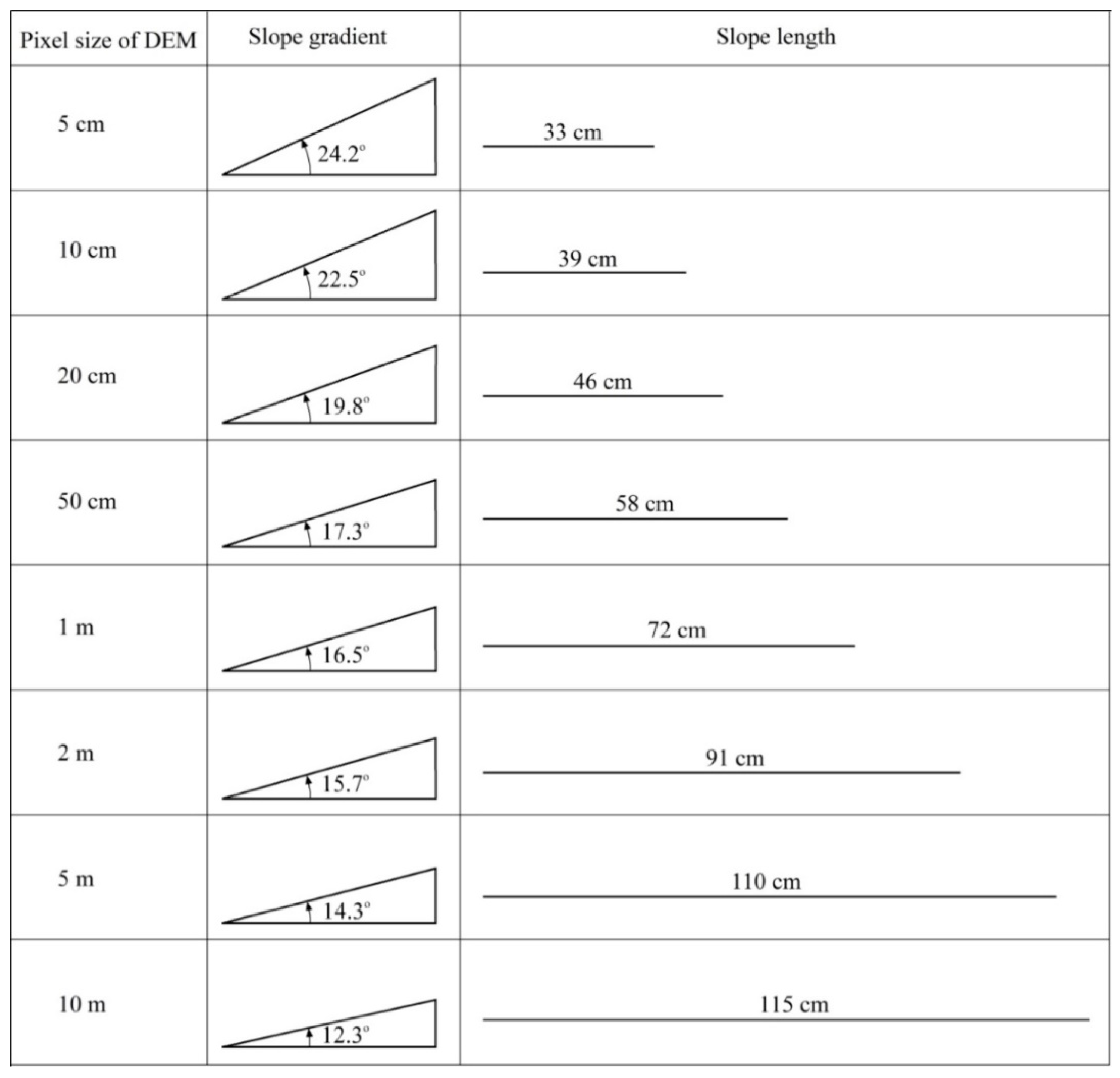
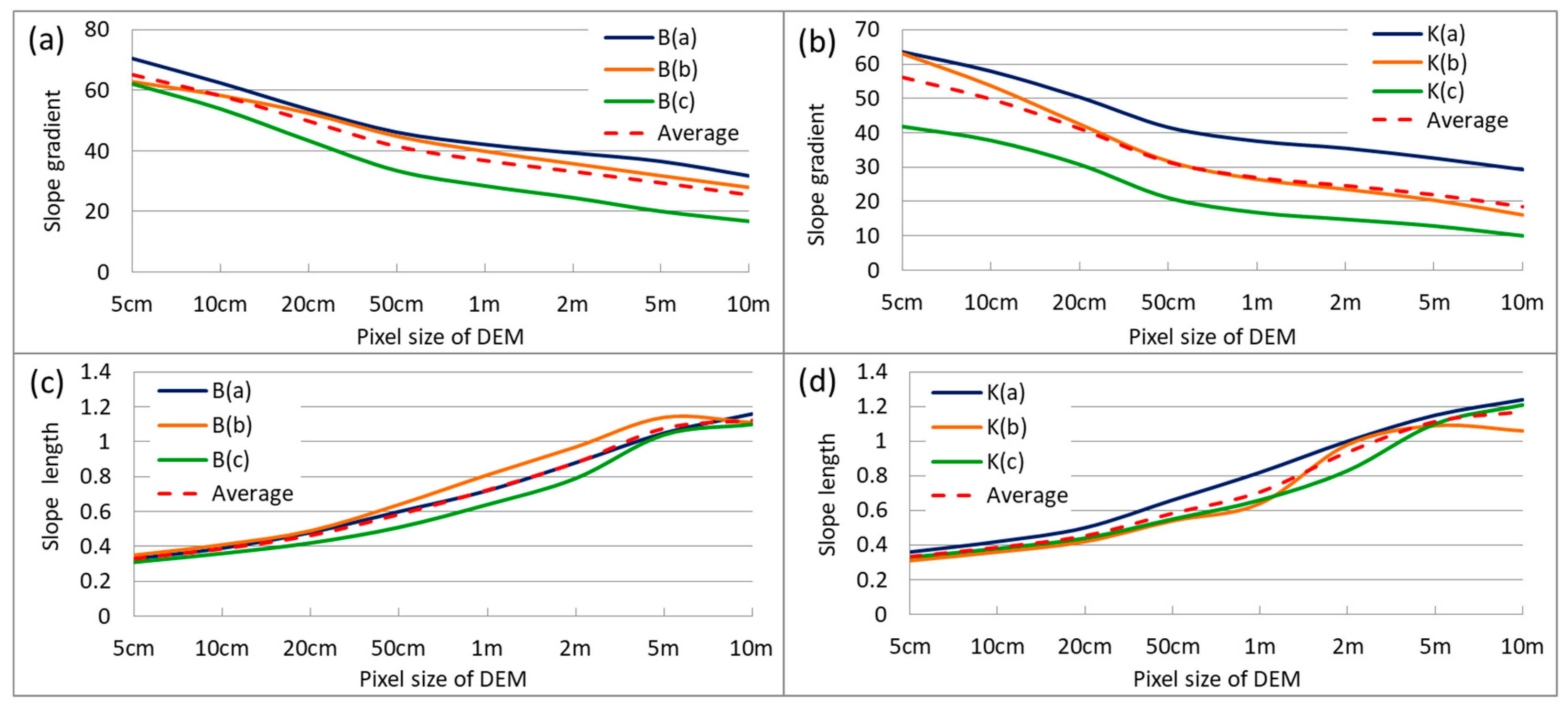
3.1. Slope Gradient and Slope Length

As shown in the Figure 2a, there is a decreasing trend of slope gradient with the increase in pixel size of DEM data in rain-fed plots. The plots B(a) and B(c) exhibit similar changing pattern, but the change rate is a slightly more in plot B(c) as compared to plot B(a). Plot B(b) has the lowest change rate.
Statistically, the total change in slope gradient in plot B(c) is 45.3 (73%), which is the highest, and the lowest is in plot B(b) with the difference of 34.9 (55.5%) (Table 1). More than 71% of the total change in the average line of the rain-fed plots happens during the changes in DEM data from 5 × 5 cm to 1 × 1 m. Thus, the change rate of the slope gradient is relatively higher from 5 × 5 cm to 1 × 1 m and with a slight increase from 1 × 1 to 10 × 10 m.
Comparatively, a similar decreasing trend was detected for the irrigated plots as shown in Figure 2b. The decreasing trend of slope gradient of plot K(a) and K(c) are nearly parallel. The values of total decrease in slope gradient in K(a) and K(c) are 34.3 and 31.8, respectively. The amount of change is lower than that of plot K(b), which has a total decrease of 46.9. The average change in slope gradient of the irrigated plots is 37.7, which is a little smaller than the average change in rain-fed plots (39.6). Similarly, the rate of change in the slope gradient is higher for the estimates using DEM data with the pixel size smaller than 1 × 1 m than that of coarse resolution such as 2 × 2, 5 × 5, and 10 × 10 m. In average, the variation in slope gradient of irrigated plots with the DEM resolution from 5 × 5 cm to 1 × 1 m occupies 77.5% of the total change.
In contrast to the variation pattern of slope gradient, the changing trend of slope length shows a positive trend with the increase in DEM pixel size. Unlike the obvious differences among different plots for the slope gradient, there are no significant differences in the changing trend of slope length among rain-fed and irrigated plots (Figure 2c,d). The plot K(b) has an undulating trend of change as compared to other plots. In the irrigated plots, there is a slow increase in the average value from 5 × 5 to 20 × 20 cm, and it starts to increase rapidly until 5 × 5 m pixel size. The average increasing rate of slope length is higher between 20 × 20 cm to 5 × 5 m, which occupies 78.1% of the total change (Table 1).
In addition to presenting the estimates of slope gradient and length with different DEM resolutions, a power function can be used to fit the changing pattern of slope gradient against DEM pixel size (Figure 3a). The decreasing trend is gradually stable with the increase in DEM pixel size. The slope gradients of the irrigated plots are systematically lower than those of the rain-fed plots. Comparatively, the changing trend of slope length with the increase in pixel size presents a logarithmic trend rather than a power trend (Figure 3b). The rain-fed and irrigated plots show quite a similar pattern. For both variables, the most obvious changes are observed at the pixel size, which ranges from 5 × 5 cm to 2 × 2 m.
For better understanding of this influence, an example of the slope gradient and the slope length estimates was shown in Figure 4; with the DEM data aggregated into different resolutions, the slope gradient and the slope length of the study area can be mapped. An average slope gradient was derived at 24.2° using 5 × 5 cm pixel size of DEM, while the slope gradient decreased along with the increase in the pixel size of DEM; finally, the slope gradient was found to be only 12.2° in the 10 × 10 m pixel size DEM. Nearly half of the slope gradient has decreased from 5 × 5 cm to 10 × 10 m pixel sizes of DEM. Thus, it is clear that there is a significant decrease on slope gradient with increase in the pixel size of DEM. The slope length is also an important factor effecting the soil erosion rate, although it has a smaller effect than the slope gradient [46]. Thus, it is also important to know how a slope length changes with changing DEM resolution. Values of derived slope length using different resolution DEM is quite inverse to the slope gradient. The slope length increases with the increase in pixel size of DEM. The average slope length was only 33 cm in 5 × 5 cm pixel size of DEM, while it measured 115 cm in 10 × 10 m pixel size, which is a nearly three and half times increase when the pixel sizes increased from 5 × 5 cm to 10 × 10 m of DEM. This is a clear indication of high sensitivity of DEM resolution to the derivation of the slope gradient, the slope length, and the topographic factor.

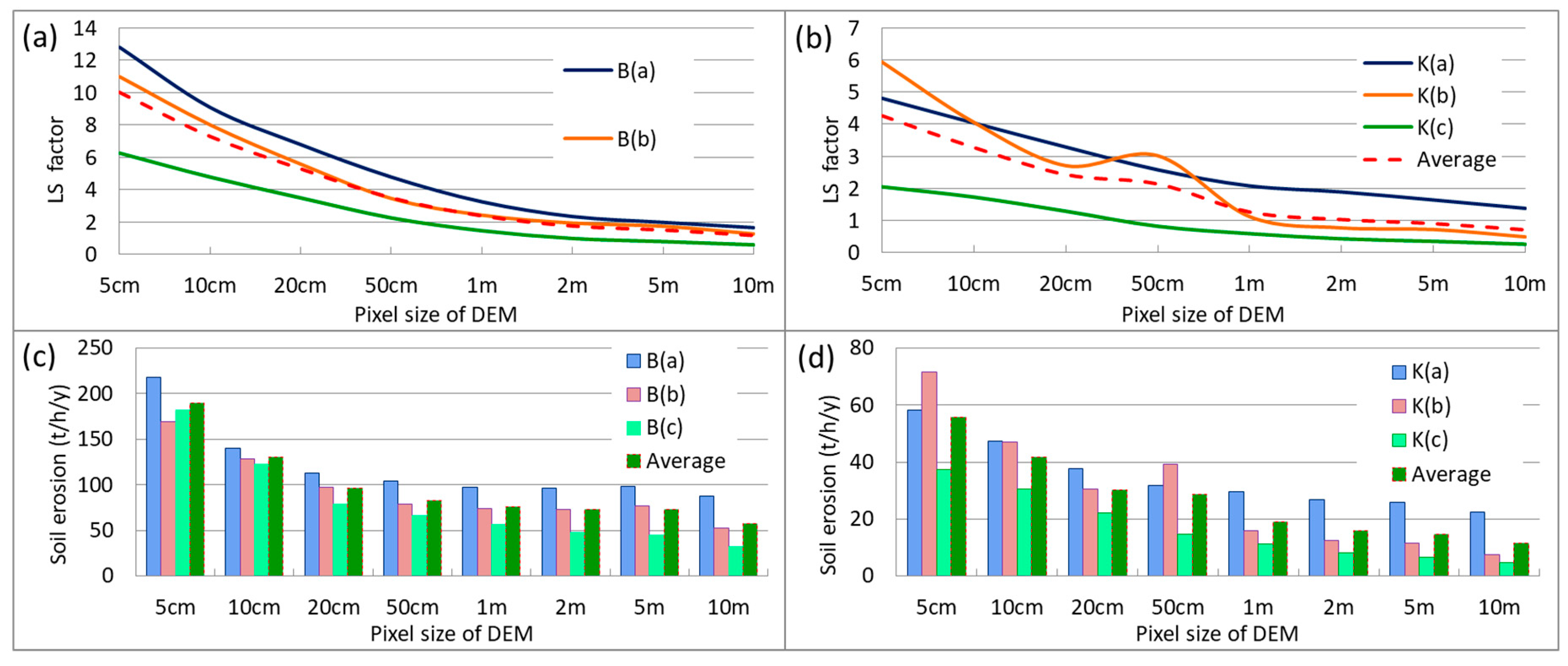
3.2. LS Factor and Soil Erosion

It is evident from above that the DEM pixel size has a positive relation with the slope length and inverse relation with slope gradient. According to the Equation (2), the LS factor shows a decreasing trend, as shown in Figure 5a,b. There are smooth decreasing trends for the estimated LS factors in all rain-fed plots. However, it is highly fluctuating in the irrigated plot K(b) due to the high fluctuation of slope length. The average changing rate of LS factor of rain fed plots is higher than that of irrigated plots.
The average LS factor of the rain-fed plots has decreased 88.3% when using the DEM data with spatial resolution from 5 × 5 cm to 10 × 10 m. For the irrigated plots, the change is measured at −83.4% (Table 2). There are higher shrinking rates of LS factor from 5 × 5 cm to 1 × 1 m pixel size of DEM in all plots (including rain-fed and irrigated). There is more than an 80% reduction in the value of LS factor in these pixel sizes of DEM. The estimates of the LS factor show high sensitivity to the use of high-resolution (≤1 × 1 m) DEM data than those with coarse resolution (≥1 × 1 m).
With the estimated LS factor, combined with other factors, the soil erosion of each plot was estimated with the average value at different spatial resolutions. As shown in Figure 5c,d, there is a visible decreasing trend in soil erosion with the increase in the DEM pixel size. For the rain-fed and irrigated plots, the variation of soil erosion at different DEM pixel sizes is mainly controlled by the LS factor because of similar soil properties and rainfall conditions. Statistically, more than 90% variation of the amount of soil erosion was determined by LS factor in all individual plots at 1% significance level. Therefore, the soil erosion presents a decreasing trend for all plots with the increase in DEM pixel size.
It is evident from the Table 2 that the average amount of soil erosion of the rain-fed plots is 189.7 t/h/y when using DEM data at 5 × 5 cm pixel size. The value decreases to 57.4 t/h/y at 10 × 10 m pixel size with the reduction of 132.2 t/h/y (69.72 % decreases). Comparatively, the average soil erosion of the irrigated plots is much lower as compared to the rain-fed plots due to the differences in the topographic and C factor. The average soil erosion rate of the irrigated plot is 56 t/h/y when using 5 × 5 cm DEM data, and it changes to 11 t/h/y at 10 × 10 m pixel size. The total decrease is 44.1 t/h/y, and in percentage terms, it accounts for 79.3%. The soil erosion estimates of plot K(b) reflect the impact from the fluctuation of the LS factor. For the irrigated plots, an 83% decrease was contributed by 5 × 5 cm to 1 × 1 m pixel size of DEM in total decrease, and different plots have different proportions of contribution ranging from 80 to 87%. A decreasing rate of soil erosion with the increase in DEM pixel size is higher in the irrigated plots compared to the rain-fed plots. The decreasing rate of soil erosion with the increasing DEM pixel sizes is quite higher in irrigated plots as compared to the rain-fed plots because of the higher modification of parent slopes in irrigated plots as compared to the rain-fed one.
The trend lines for the average values of the LS factor and the soil erosion against the DEM pixel size present a similar changing pattern in both the rain-fed and irrigated plots (Figure 6a,b). A power function can be used to express the relationship. Although the function values are different for the same pixel size, all functions indicate that the decrease in the values of LS factor and soil erosion mainly happens in the range of pixel size from 5 × 5 cm to 2 × 2 m with the increase in DEM pixel size. When the pixel size is larger than 1 × 1 m, changes in LS factor and soil erosion become very slow.

4. Discussion

4.1. Impact of DEM Resolution on Topographic Factors

The DEM is the primary data source used for depicting surface information, which provides fundamental information for wide applications in land surface processes and environmental analysis [51,52]. In this study, the impact from the spatial resolution of DEM data has clearly reflected by the estimation of the LS factor. The spatial resolution of DEM data determines the accuracy of topographic reality, which cannot be detected with coarse resolution DEM data by missing the complexities of landform and often skipping important details of land surface [53,54]. Therefore, there were significant changes in the values of the topographic factors with the change in the spatial resolution of DEM data and the computation accuracy of the LS factor, which decreased with the increase in DEM pixel size [55]. A higher accuracy of hydrological modeling was derived by using higher resolution DEM data as compared to the use of coarse resolution DEM [19,21,22,23]. The calculation of the LS factor using the DEM data with the pixel size ranging from 1 × 1 m to 90 × 90 m over a Burnt National Park in New South Wales, Australia, had revealed that a higher resolution DEM gives closer values to the measured values of the plots. Nevertheless, freely available low-resolution DEM is not able detect micro-complexities of topographic surface such as hill slope agriculture terraces in Nepal.
The recent advent of UAV-derived images combined with computer-based powerful photogrammetric system has improved data accuracies and provides large-scale database for small area studies [28], by which it became possible to detect more accurate and detail topographic surface information of hill slope agriculture terraces of Nepal. Although the past studies used coarser resolution DEM data as compared to present study, the changing trend of slope gradient, slope length, and topographic factors were similar with the changes in DEM resolution [56,57]. However, there were no findings revealed in this study by using the DEM resolution as high as 5 × 5 cm. Meanwhile, an important phenomenon was found that the change in the rate of LS factor is quite high, while using DEM data with pixel size below 50 × 50 cm. The result indicates that this high-resolution DEM can detect micro-topographic roughness, which was impossible in the past studies.
This study presents variations over several topographic complexities of terraced agriculture plots, including both rain-fed and irrigated plots. It partly increases the reliability of the finding through the comparative study. Generally, the average slope gradient of rain-fed plots is quite high as compared to irrigated plots, because they are made at steeper slope as compared to the irrigated plots in the study area. A total change in slope gradient is higher in rain-fed plots, but inversely, the rate of change is higher in irrigated plots because of irrigated plots strictly follow the contour when making terraces, but it is roughly followed in rain-fed plots. A sharp decrease in LS factor is recovered more in the rain-fed terraces as compared to that of the irrigated plots when using DEM data with a pixel size of 5 × 5 cm and 10 × 10 cm used. It is attributed to the big amount of roughness of the rain-fed cultivated surface due to recent tillage of cultivated surface of rainfed terraces and comparatively smooth surface in irrigated terraces. The higher rate of change in topographic factors in higher resolution DEM is resulted in due to detection of micro-topographic roughness of surfaces by high resolution DEM. In general, the identification of power function shows the changing trend of slope gradient and LS factor and logarithmic changing trend of slope length against spatial resolution DEM. It is the most important findings of the present study that were made possible by UAV-derived high-resolution DEM. More importantly, the changing trends are becoming stable when the DEM resolution is above 2 × 2 m, which partly indicates that this resolution is a threshold value for topographic calculation and estimate soil erosion of narrow cultivated terraces.

4.2. Impact of DEM Resolution on Estimated Soil Loss

It is well known that rainfall and topography are the most dominant controlling factors of soil erosion. In this study area, there are no significant differences in the values of rainfall erosivity and soil erodibility. Thus, the differences of soil erosion rates in different plots are highly controlled by a topographic factor. Soil erosion has a linear relationship with the slope gradient and the slope length because the velocity of runoff increases with the increase in slope gradient and slope length. The increase in flow depth associated with the runoff accumulation at the downslope, which increases the erosion power [58,59]. Therefore, the soil erosion estimation requires reliable DEM data, and the spatial resolution is an important aspect [57]. Although previous analysis has identified the decreasing trend of soil erosion with the decrease in spatial resolution of DEM [11,17,58,60,61], this study presents a similar study with the DEM resolution as high as 5 × 5 cm and identifies the changing pattern of soil erosion rate with the variation of DEM resolution from 5 × 5 cm to 10 × 10 m.
As shown in Figure 6, the changing rates of the estimated soil erosion are quite high in the resolution ranges from 5 × 5 cm to 1 × 1 m because of the detection of micro-topographic surface of high-resolution DEM and sharp diminish of micro-topographic roughness as DEM resolution decreases. The generalization of micro-topographic surface with the decrease in DEM resolution greatly reduces the estimated rates of soil erosion. The higher rate of soil erosion in rain-fed plots as compared to irrigated plots is due to the higher slope gradient. Meanwhile, the decreasing rate of soil erosion in the rain-fed terraces is bigger than those of the irrigated ones between the pixel sizes of DEM from 5 × 5 to 10 × 10 cm is due to the higher change rate of LS factor. The detection of micro level variation of soil erosion rates was made possible by high resolution DEM in narrow agriculture terraces in the hill slope. With the increase in the DEM pixel size, the DEM data cannot depict micro level variations.
In addition to the general variation pattern, the identification of the power function to express the changing trend of soil erosion against spatial resolution of DEM is the most important finding of the present study. This study revealed that the DEM data are not able to detect the micro-topographic modification of natural slopes and accurately estimate soil erosion rate when the pixel sizes of DEM are bigger than two meters. The higher accuracy of soil erosion can be derived by using the smaller pixel size of DEM but actual soil erosion process in such a micro-topographic rough surface is still unknown because there is a lack of empirical studies using such a high-resolution DEM up to 5 × 5 cm pixel size comparing with measured data of soil loss. Thus, it needs further verification with measured values.

4.3. Implication from the Estimation of Soil Erosion Rate at a High-Resolution Level

This study is not concerned to actual soil erosion rate rather than a sensitivity analysis of estimated soil erosion rates with DEM resolution change, but it is equally important to note how far the estimated soil erosion rates are near to reality. Thus, the discussion of soil erosion rates in different parts of the world in general and in Nepal in particular will be supportive information for estimation validity. Variation of soil erosion rates in different places are due the variation of different controlling factors. Among these factors rainfall and topography are the most dominant physical factors [62]. Mountainous cropland areas with high rainfall intensity in developing countries have the higher soil erosion rates as compared to developed countries due to poor land management practices [11,63,64,65]. The study revealed that soil erosion rates are higher in traditional agriculture areas of developing countries in the world [4] than their counter parts in developed world.
In Nepal, field measurement of soil erosion rates in Likhu Khola watershed in the central part of Middle Hill region of Nepal was 2.7 to 12.9 t/h/y, where the annual rainfall was 2141 mm [13]. Similarly, the soil erosion rate was 0.6 to 14 t/h/y in outward sloping terraces in the northeast part of Kathmandu (Nagarkot) and up to 35 t/h/y soil erosions in inward sloping red soil terraces in Pokhara and Jikhu Khola with up to 20 t/h/y [66]. There are strong variations of soil erosion rate in the hill slope agricultural area due to the variation of rainfall intensity, topography, management practices, and soil types. The government data indicate that soil erosion rates in the degraded forest and agriculture land in the central part of Middle Hill region were 31.5 to 140 t/h/y [67]. Compared with the above measurements in the hill slope terraces of Nepal, the estimates of soil erosion rate in this study are reasonably higher because of the higher rainfall intensity in the study area and detection of actual land surface of narrow agriculture terraces by high resolution DEM.
In addition to measured values, there are several estimates of soil erosion rate of different parts of Nepal using medium (30 × 30 m) to coarse (90 × 90 m) resolutions DEM [41,42,44,68,69,70]. The use of medium to coarse resolution DEM data and relatively small rainfall of the study areas induced the low amount of soil erosion estimates. In comparison, this study detected higher soil erosion rates because of the high-resolution DEM data, which can detect the micro-variability of terraces and structures of surfaces. Furthermore, it revealed how sensitivity is the estimation of soil erosion to DEM resolution. The uncertainty behind previous estimates should be considered in future soil erosion assessment. Further investigation using various resolution DEM in various surface roughness areas is required for the identification of suitable DEM size for a particular area. Finally, according to the characteristic of RUSLE model, it covers only sheet and rill erosion, which do not cover the gully erosion. Protection channels are made by farmers to protect their farm plots by gully erosion during torrential rainfall. Thus, it is not so serious for the gully erosion in the study plots. However, sometimes they fail to fully protect their farmland due to various limitations. Thus, it requires further investigation including gully erosion using high resolution DEM with the verification of actual measured data.

5. Conclusions

The spatial resolution of topographic data is one of the most important determinants for accurately estimating soil erosion rate in the hill slope agriculture terraces by controlling the accuracy of slope gradient and slope length. Therefore, the spatial resolution of DEM data is an important issue for modeling and estimation. Currently, most of the freely available DEMs are medium (30 × 30 m) to coarse (90 × 90 m) resolutions, which are unable to detect micro-topographic features modified by farmers in the hill slope for crop cultivation.
A higher relationship between spatial resolution of DEM and topographic factors of agriculture terraces in the hill slopes of Nepal was found. A higher rate of change was found in higher resolution DEM rather than lower resolution. It indicates that higher resolution DEM is suitable to derive a real topographic factor. There were differences in the changing values of topographic factors in rain-fed terraces and irrigated ones, the trend of topographic values is found to be similar. There is a negative power trend relationship of slope gradient with spatial resolution of DEM, but slope length has positive logarithmic relationship with DEM resolution. The LS factor and the soil erosion rates also have a negative power trend relationship with the spatial resolution of DEM. The changing trend of soil erosion was highly controlled by topographic factors in the study area rather than other factors such as rainfall erosivity and C factor. Hence, there was uniform relation of the changing trend of estimated soil erosion with DEM resolution as with LS factor.
This study concluded that DEM resolution is highly sensitive in land surface analysis for geomorphic processes and hydrological modeling. The DEM resolution less than 2 × 2 m pixel size cannot detect the narrow agriculture terraces of hill slope areas, and it cannot detect the actual rate of soil erosion. In contrast, the DEM data with the pixel size from 5 × 5 to 50 × 50 cm can depict topographic factors and soil erosion rates with high variability. Behind the changing mechanism of soil erosion estimates with different DEM resolutions, this case study well indicates the importance of the DEM resolution for soil erosion estimation for hill slope agriculture terraces in Nepal. Estimated soil erosion rates of the study can be further validated with field measured data, which are the main remaining gap of this study.

Author Contributions

Conceptualization, Chhabi Lal Chidi.; methodology, Chhabi Lal Chidi and Wei Zhao; software, Chhabi Lal Chidi and Suresh Chaudhary; validation, Wei Zhao, Donghong Xiong, and Yanhong Wu; investigation, Chhabi Lal Chidi and Suresh Chaudhary; resources, Chhabi Lal Chidi and Suresh Chaudhary; draft manuscript preparation, Chhabi Lal Chidi; comments and suggestion, Wei Zhao, Donghong Xiong, Yanhong Wu, and Suresh Chaudhary; final manuscript, Chhabi Lal Chidi and Wei Zhao. All authors have read and agreed to the published version of the manuscript.

Funding

This study was supported by, the External Cooperation Program of BIC of Chinese Academy of Sciences, the National Natural Science Foundation of China (No. 41771409), the Sichuan Science and Technology Program (No. 2020JDJQ0003), and the Kathmandu Center for Research and Education CAS-TU.

Data Availability Statement

The data presented in this study are available on request from the corresponding author.

Acknowledgments

The authors would like to thank to Nara Sagar Shrestha, permanent resident of Kirtipur, Kathmandu for language correction and the local peoples of the study area who involved during the field investigation.

Conflicts of Interest

The authors declare no conflict of interest.

References

  1. Acharya, A.K.; Kafle, N. Land degradation issues in Nepal and its management through agroforestry. J. Agric. Environ. 2009, 10, 115–123. [Google Scholar] [CrossRef]
  2. Chalise, D.; Kumar, L.; Kristiansen, P. Land degradation by soil erosion in Nepal: A review. Soil Syst. 2019, 3, 12. [Google Scholar] [CrossRef] [Green Version]
  3. Montgomery, D.R. Soil erosion and agricultural sustainability. Proc. Natl. Acad. Sci. USA 2007, 104, 13268–13272. [Google Scholar] [CrossRef] [PubMed] [Green Version]
  4. Borrelli, P.; Robinson, D.A.; Fleischer, L.R.; Lugato, E.; Ballabio, C.; Alewell, C.; Meusburger, K.; Modugno, S.; Schütt, B.; Ferro, V.; et al. An assessment of the global impact of 21st century land use change on soil erosion. Nat. Commun. 2017, 8, 1–13. [Google Scholar] [CrossRef] [PubMed] [Green Version]
  5. Cheng, H. Future Earth and Sustainable Developments. The Innovation 2020, 1, 100055. [Google Scholar] [CrossRef]
  6. Wei, K.; Ouyang, C.; Duan, H.; Li, Y.; Chen, M.; Ma, J.; An, H.; Zhou, S. Reflections on the catastrophic 2020 Yangtze River Basin flooding in southern China. The Innovation 2020, 1, 100038. [Google Scholar] [CrossRef]
  7. Peduzzi, P. Flooding: Prioritizing protection? Nat. Clim. Chang. 2017, 7, 625–626. [Google Scholar] [CrossRef]
  8. Panagos, P.; Borrelli, P.; Meusburger, K. A new European slope length and steepness factor (LS-Factor) for modeling soil erosion by water. Geosciences 2015, 5, 117–126. [Google Scholar] [CrossRef] [Green Version]
  9. Chow, T.L.; Rees, H.W.; Daigle, J.L. Effectiveness of terraces grassed waterway systems for soil and water conservation: A field evaluation. J. Soil Water Conserv. 1999, 54, 577–583. [Google Scholar]
  10. Chapagain, T.; Raizada, M.N. Agronomic challenges and opportunities for small holders terrace agriculture in developing countries. Front. Plant Sci. 2017, 8, 1–15. [Google Scholar] [CrossRef] [Green Version]
  11. Panagos, P.; Borrelli, P.; Poesen, J.; Ballabio, C.; Lugato, E.; Meusburger, K.; Montanarella, L.; Alewell, C. The new assessment of soil loss by water erosion in Europe. Environ. Sci. Policy 2015, 54, 438–447. [Google Scholar] [CrossRef]
  12. Malla, U.M.; Chidi, C.L. Indigenous practice of natural resource management at Pipaldanda, Palpa. Himal. Rev. 1997, 24, 36–49. [Google Scholar]
  13. Gardner, R.A.M.; Gerrard, A.J. Runoff and soil erosion on cultivated rain fed terraces in the Middle Hills of Nepal. Appl. Geogr. 2003, 23, 23–45. [Google Scholar] [CrossRef]
  14. Basso, B. Digital terrain analysis: Data source, resolution and applications for modeling physical processes in agroecosystems. Riv. Ital. Agrometeorol. 2005, 2, 5–14. [Google Scholar]
  15. Gregar, J. Understanding soil erosion by water to improve soil conservation. Crops Soils Mag. 2020. [Google Scholar] [CrossRef]
  16. Lin, S.; Jing, C.; Coles, N.A.; Chaplot, V.; Moore, N.J.; Wu, J. Evaluating DEM source and resolution uncertainties in the Soil and Water Assessment Tool. Stoch. Environ. Res. Risk Assess. 2013, 27, 209–221. [Google Scholar] [CrossRef]
  17. Mondal, A.; Khare, D.; Kundu, S.; Mukharjee, S.; Mukhopadhyay, A.; Mondal, S. Uncertainty of soil erosion modelling using open source high resolution and aggregated DEMs. Geosci. Front. 2017, 8, 425–436. [Google Scholar] [CrossRef] [Green Version]
  18. Shan, Z.; Yang, X.; Zhu, Q. Effects of DEM resolutions on LS and hillslope erosion estimation in a burnt landscape. Soil Res. 2019, 57, 797–804. [Google Scholar] [CrossRef]
  19. Azizian, A.; Brocca, L. Determining the best remotely sensed DEM for flood inundation mapping in data sparse regions. Int. J. Remote Sens. 2020, 41, 1884–1906. [Google Scholar] [CrossRef]
  20. Lin, K.; Zhang, Q.; Chen, X. An evaluation of impacts of DEM resolution and parameter correlation on TOPMODEL modeling uncertainty. J. Hydrol. 2010, 394, 370–383. [Google Scholar] [CrossRef]
  21. Nagaveni, C.; Kumar, K.P.; Ravibabu, M.V. Evaluation of TanDEMx and SRTM DEM on watershed simulated runoff estimation. J. Earth Syst. Sci. 2019, 128, 2. [Google Scholar] [CrossRef] [Green Version]
  22. Song, J.; Goda, K. Influence of elevation data resolution on tsunami loss estimation and insurance rate-making. Front. Earth Sci. 2019, 7, 246. [Google Scholar] [CrossRef]
  23. Suliman, A.H.A.; Gumindoga, W.; Awchi, T.A.; Katimon, A. DEM resolution influences on peak flow prediction: A comparison of two different based DEMs through various rescaling techniques. Geocarto Int. 2019, 1–14. [Google Scholar] [CrossRef]
  24. Watson, C.S.; Kargel, J.S.; Tiruwa, B. UAV-derived Himalayan topography: Hazard assessments and comparison with Global DEM products. Drones 2019, 3, 18. [Google Scholar] [CrossRef] [Green Version]
  25. Jeziorska, J. UAS for wetland mapping and hydrological modeling. Remote Sens. 2019, 11, 1997. [Google Scholar] [CrossRef] [Green Version]
  26. Langhammer, J.; Vackova, T. Detection and mapping of the geomorphic effects of flooding using UAV photogrammetry. Pure Appl. Geophys. 2018, 175, 3223–3245. [Google Scholar] [CrossRef]
  27. Siqueira Junior, P.; Silva, M.L.N.; Cândido, B.M.; Avalos, F.A.P.; Batista, P.V.G.; Curi, N.; Lima, W.; Quinton, J.N. Assessing water erosion processes in degraded area using unmanned aerial vehicle imagery. Rev. Bras. Cienc. Solo 2019, 43, e0190051. [Google Scholar] [CrossRef]
  28. Uysal, M.; Toprak, A.S.; Polat, N. DEM generation with UAV photogrammetry and accuracy analysis in Sahitler hill. Measurement 2015, 73, 539–543. [Google Scholar] [CrossRef]
  29. Abdullah, Q.; Bethel, G.; Hussain, M.; Munjy, R. Photogrammetric project and mission planning. In Manual of Photogrammetry; McGlone, G.C., Ed.; American Society for Photogrammetry and Remote Sensing: Bethesda, MD, USA, 2013; pp. 1187–1220. [Google Scholar]
  30. Kraus, K.; Harley, I.A.; Kyle, S. Photogrammetry: Geometry from Images and Laser Scans (de Gruyter Textbook), 2nd ed.; Walter de Gruyter: New York, NY, USA, 2007. [Google Scholar]
  31. Bemis, S.P.; Micklethwaiteb, S.; Turner, D.; James, M.R.; Akciz, S.; Thiele, S.T.; Bangash, H.A. Ground-based and UAV-Based photogrammetry: A multi-scale, high-resolution mapping tool for structural geology and paleoseismology. J. Struct. Geol. 2014, 69, 163–178. [Google Scholar] [CrossRef]
  32. Gindraux, S.; Boesch, R.; Farinotti, D. Accuracy assessment of Digital Surface Models from Unmanned Aerial Vehicles’ imagery on glaciers. Remote Sens. 2017, 9, 186. [Google Scholar] [CrossRef] [Green Version]
  33. Rock, G.; Ries, J.B.; Udelhoven, T. Sensitivity analysis of UAV-photogrammetry for creating Digital Elevation Models (DEM). In Proceedings of the International Archives of the Photogrammetry, Remote Sensing and Spatial Information Sciences, Volume XXXVIII-1/C22., 2011 ISPRS Zurich 2011 Workshop, Zurich, Switzerland, 14–16 September 2011. [Google Scholar]
  34. Rusli, N.; Majid, M.R.; Razali, N.F.A.A.; Yaacob, N.F.F. Accuracy assessment of DEM from UAV and TanDEM-X imagery. In Proceedings of the 2019 IEEE 15th International Colloquium on Signal Processing & Its Applications (CSPA 2019), Penang, Malaysia, 8–9 March 2019. [Google Scholar]
  35. Rogers, S.R.; Manning, I.; Livingstone, W. Comparing the spatial accuracy of Digital Surface Models from four unoccupied aerial systems: Photogrammetry versus LiDAR. Remote Sens. 2020, 12, 2806. [Google Scholar] [CrossRef]
  36. Cogliati, M.; Tonelli, E.; Battaglia, D.; Scaioni, M. Extraction of DEMs and orthoimages from archieve aerial imagery to support project planning in civil engineering. In Proceedings of the ISPRS Annals of the Photogrammetry, Remote Sensing and Spatial Information Sciences, Volume IV-5/W1, Geospace 2017, Kyiv, Ukraine, 4–6 December 2017. [Google Scholar]
  37. Seitz, S.M.; Curless, B.; Diebel, J.; Scharstein, D.; Szeliski, R. A comparison and evaluation of multi-view stereo reconstruction algorithms. In Proceedings of the 2006 IEEE Computer Society Conference on Computer Vision and Pattern Recognition (CVPR’06), New York, NY, USA, 17–22 June 2006; Volume 1. [Google Scholar]
  38. Wang, R.; Zhang, S.; Pu, L.; Yang, J.; Yang, C.; Chen, J.; Guan, C.; Wang, Q.; Chen, D.; Fu, B.; et al. Gully erosion mapping and monitoring at multiple scales based on multi-source remote sensing data of the Sancha River Catchment, Northeast China. ISPRS Int. J. Geo-Inf. 2016, 5, 200. [Google Scholar] [CrossRef] [Green Version]
  39. Coz, M.L.; Delclaux, F.; Guillaume, P.; Favreau, G. Assessment of Digital Elevation Model (DEM) aggregation methods for hydrological modeling: Lake Chad basin, Africa. Comput. Geosci. 2009, 35, 1661–1670. [Google Scholar] [CrossRef]
  40. Bian, L.; Butler, R. Comparing Effects of aggregation methods on statistical and spatial properties of simulated spatial data. Photogramm. Eng. Remote Sens. 1999, 65, 73–84. [Google Scholar]
  41. Chalise, D.; Kumar, L. Land use change affects water Eros. in the Nepal Himalayas. PLoS ONE 2020, 15, e0231692. [Google Scholar] [CrossRef] [PubMed] [Green Version]
  42. Koirala, P.; Thakuri, S.; Joshi, S.; Chauhan, R. Estimation of soil erosion in Nepal using a RUSLE modeling and geospatial tool. Geosciences 2019, 9, 147. [Google Scholar] [CrossRef] [Green Version]
  43. Renard, K.G.; Foster, G.R.; Weesies, G.A.; Porter, J.P. RUSLE: Revised universal soil loss equation. J. Soil Water Conserv. 1991, 46, 30–33. [Google Scholar]
  44. Uddin, K.; Murthy, M.S.R.; Wahid, S.M.; Matin, M.A. Estimation of soil erosion dynamics in the Koshi Basin using GIS and remote sensing to assess priority areas for conservation. PLoS ONE 2016, 11, e0150494. [Google Scholar] [CrossRef] [Green Version]
  45. Ganasri, B.P.; Gowda, R. Assessment of soil erosion by RUSLE model using remote sensing and GIS—A case study of Nethravathi Basin. Geosci. Front. 2016, 7, 953–961. [Google Scholar] [CrossRef] [Green Version]
  46. Morgan, R.P.; Davidson, D.A. Soil Erosion and Conservation; Longman Group: London, UK, 1991. [Google Scholar]
  47. Wallis, C.; Watson, D.; Tarboton, D.; Wallace, R. Parallel flow-direction and contributing area calculation for hydrology analysis in digital elevation models. In Proceedings of the ADPTA09′ International Conference on Parallel and Distributed Processing Technique and Applicationa, Las Vegas, NV, USA, 13–16 July 2009. [Google Scholar]
  48. USDA. Soil Survey Manual; United State Department of Agriculture: Washngton, DC, USA, 1951.
  49. Li, X.I.; Wu, B.; Zhang, L. Dynamic monitoring of soil erosion for upper stream of Miyun Reservoir in the last 30 years. J. Mt. Sci. 2013, 10, 801–811. [Google Scholar] [CrossRef]
  50. Meng, E.C.H.; Hu, R.; Shi, X.; Zhang, S. Maize in China: Production Systems, Constraints, and Research Priorities; CIMMYT: Texcoco, Mexico, 2006. [Google Scholar]
  51. Claessens, L.; Heuvelink, G.B.; Schoorl, J.M.; Veldkamp, A. DEM resolution effects on shallow landslide hazard and soil redistribution modeling. Earth Surf. Process. Landf. 2005, 30, 461–477. [Google Scholar] [CrossRef]
  52. Schoorl, J.M.; Sonneveld, M.P.; Veldkamp, A. Three-dimensional landscape process modelling: The effect of DEM resolution. Earth surface processes and landforms. J. Br. Geomorphol. Res. Group 2000, 25, 1025–1034. [Google Scholar]
  53. Szyputa, B. Digital elevation models in geomorphology. Hydro-Geomorphol. Model Trends 2017, 81–112. [Google Scholar] [CrossRef] [Green Version]
  54. Wang, S.Y.; Zhu, X.L.; Zhang, W.B.; Yu, B.; Fu, S.H.; Liu, L. Effect of different topographic data sources on soil loss estimation for a mountainous watershed in Northern China. Environ. Earth Sci. 2016, 75, 1382. [Google Scholar] [CrossRef]
  55. Lu, S.; Liu, B.; Hu, Y.; Fu, S.; Cao, Q.; Shi, Y.; Huang, T. Soil erosion topographic factor (LS): Accuracy calculated from different data sources. Catena 2019, 187, 104334. [Google Scholar] [CrossRef]
  56. Zhang, H.; Baartman, J.E.M.; Yang, X.; Gai, L.; Geissen, V. Influence of terraced area DEM resolution on RUSLE LS factor. In Proceedings of the Geophysical Research Abstracts, EGU General Assembly, Vienna, Austria, 23–28 April 2017. [Google Scholar]
  57. Zhang, H.; Yang, Q.; Wang, M.; Yang, J.; Jin, B. Analysis of DEM resolution on erosional terrain characteristics of terrace area. Nongye Jixie Xuebao/Trans. Chin. Soc. Agric. Mach. 2017, 48, 172–179. [Google Scholar] [CrossRef]
  58. Fu, S.; Cao, L.; Liu, B.; Wu, Z.; Savabi, M.R. Effects of DEM grid size on predicting soil loss from small watersheds in China. Environ. Earth Sci. 2015, 73, 2141–2151. [Google Scholar] [CrossRef]
  59. Pennock, D. Soil Erosion: The Greatest Challenge for Sustainable Soil Management; Food and Agriculture Organization (FAO): Rome, Italy, 2019. [Google Scholar]
  60. Ren, S.; Liang, Y.; Sun, B. Research on sensitivity for soil erosion evaluation from DEM and remote sensing data source of different map scales and image resolutions. Procedia Environ. Sci. 2011, 10, 1753–1760. [Google Scholar] [CrossRef] [Green Version]
  61. Saxena, A.; Jat, M.K.; Kumar, S. Uncertainty analysis of high-resolution open-source DEMs for modeling soil erosion. In Proceedings of the Roorkee Water Conclave 2020, Roorkee, India, 26–28 February 2020. [Google Scholar]
  62. FAO. Status of World Soil Resources (SWSR)—Main Report; Food and Agriculture Organization of the United Nations and Intergovernmental Technical Panel on Soils: Rome, Italy, 2015. [Google Scholar]
  63. Nguyen, X.H.; Pham, A.H. Assessing soil erosion by agricultural and forestry production and proposing solutions to mitigate: A case study in Son La Province, Vietnam. Appl. Environ. Soil Sci. 2018, 1–10. [Google Scholar] [CrossRef]
  64. Pierce, F.J.; Larson, W.E.; Dowdy, R.H.; Graham, W.A.P. Productivity of soils: Assessing long-term changes due to erosion. J. Soil Water Conserv. 1983, 38, 39–44. [Google Scholar]
  65. Xiong, M.; Sun, R.; Chen, L. A global comparison of soil erosion associated with land use and climate type. Geoderma 2019, 343, 31–39. [Google Scholar] [CrossRef]
  66. Nakarmi, G.; Schrier, H.; Merz, J.; Mathema, P. Erosion dynamics in the Jikhu and Yarsha Khola watersheds in Nepal. In Proceedings of the People and Resource Dynamics Project, Baoshan, China, 2–5 March 1999; pp. 209–217. [Google Scholar]
  67. CBS. Environmental Statistics of Nepal; Central Bureau of Statistics: Nepal, South Asia, 2019.
  68. Impat, P. Hydrometeorology and Sediment Data from the Phewa Watershed; Kathmandu HMG/UNDP/FAO/IWM Project: Kathmandu, Nepal, 1981. [Google Scholar]
  69. Sah, K.; Lamichhane, S. GIS and remote sensing supported soil erosion assessment of Kamala River Watershed, Sindhuli, Nepal. Int. J. Appl. Sci. Biotechnol. 2019, 7, 54–61. [Google Scholar] [CrossRef]
  70. Shrestha, D.P. Assessment of soil erosion in the Neapalese Himalaya, A case study in Likhu khola valley, Middle Mountain Region. Land Husb. 1997, 2, 59–80. [Google Scholar]
Figure 1. Location of the study area (a), plots location (b), and the selected six plots.
Ijgi 10 00028 g001
Figure 2. Variation of pattern of slope gradient (a,b) and slope length (c,d) of the selected plots at different digital elevation model (DEM) resolutions.
Ijgi 10 00028 g002
Figure 3. Changing trend of slope gradient (a) and slope length (b) with the variation of DEM resolution.
Ijgi 10 00028 g003
Figure 4. Derived average slope gradient and slope length by using DEM data with different pixel sizes.
Ijgi 10 00028 g004
Figure 5. LS factor (a,b) and rate of soil erosion (t/h/y) (c,d) by pixel sizes of DEM.
Ijgi 10 00028 g005
Figure 6. Changing trend of LS factor (a) and soil erosion (b) in the rain fed and irrigated plots with the variation of DEM resolution.
Ijgi 10 00028 g006
Table 1. Changes in the slope gradient and the slope length with the variation of DEM resolution.
Pixel Size Change
5 to 10 cm10 to 20 cm20 to 50 cm50 cm to 1 m1 to 2 m2 to 5 m5 to 10 m
Slope gradientPercent changes in total changeTotal changeTotal change (%)
B(a)−20.9−22.5−19.4−10.4−7.2−7.212.3−38.7−54.9
B(b)−12.9−16.8−21.8−14.3−11.7−11.411.0−34.9−55.5
B(c)−18.2−23.1−21.8−11.0−8.6−10.07.2−45.3−73.0
Rain-fed−17.5−21.1−21.0−11.8−9.1−9.510.0−39.6−60.9
K(a)−16.5−22.0−25.6−11.8−6.1−8.39.7−34.3−53.9
K(b)−20.0−23.8−23.0−11.2−6.2−6.89.1−46.9−74.4
K(c)−12.7−22.0−30.5−13.5−6.2−6.19.0−31.8−76.0
Irrigated−16.9−22.7−25.9−12.0−6.2−7.19.2−37.7−67.1
Total−17.2−21.9−23.4−11.9−7.7−8.3−9.6−38.65−63.7
Slope lengthPercent changes in total changeTotal changeTotal change (%)
B(a)7.210.814.514.519.320.513.30.83251.5
B(b)7.910.519.722.421.122.4−3.90.76217.1
B(c)6.37.611.416.519.031.67.60.79254.8
Rain-fed7.19.715.117.619.724.85.90.79240.4
K(a)6.89.118.218.220.517.010.20.88244.4
K(b)6.78.016.013.345.314.7−4.00.75241.9
K(c)5.76.812.512.519.330.712.50.88266.7
Irrigated6.48.015.514.727.521.16.80.84251.0
Total6.78.815.316.223.722.96.30.82245.7
Table 2. Change in LS factor and soil erosion with the variation of DEM resolution.
Pixel Size Change
5 to 10 cm10 to 20 cm20 to 50 cm50 cm to 1 m1 to 2 m2 to 5 m5 to 10 m
LSfactorPercent changes in total changeTotal changeTotal change (%)
B(a)33.320.618.013.78.23.23.0−11.2−87.1
B(b)30.724.921.910.65.02.04.8−9.7−88.5
B(c)26.122.721.814.08.43.43.6−5.7−90.6
Rain-fed30.822.620.212.67.12.83.8−8.9−88.3
K(a)22.421.920.714.65.57.37.6−3.4−71.3
K(b)34.524.8−5.734.96.40.94.2−5.5−91.8
K(c)17.924.626.312.88.94.55.0−1.8−87.3
Irrigated27.823.88.224.66.63.65.4−3.6−83.4
Total30.023.016.816.16.93.04.3−6.2−86.9
Soil lossPercent changes in total changeTotal changeTotal change (%)
B(a)59.820.87.15.20.7−1.17.6−129.8−59.6
B(b)35.026.715.73.80.6−3.421.5−117.0−69.1
B(c)39.629.08.76.35.62.48.4−150.0−82.4
Rain-fed44.925.710.25.22.5−0.512.0−132.2−69.7
K(a)29.827.516.85.57.72.69.9−35.7−61.4
K(b)38.025.8−13.536.25.31.76.4−64.1−89.6
K(c)20.325.823.310.39.94.75.7−32.6−87.6
Irrigated31.526.23.721.67.12.77.2−44.1−79.3
Total41.525.88.69.33.70.310.8−88.2−71.9
Publisher’s Note: MDPI stays neutral with regard to jurisdictional claims in published maps and institutional affiliations.

