The Potential of LiDAR and UAV-Photogrammetric Data Analysis to Interpret Archaeological Sites: A Case Study of Chun Castle in South-West England

Abstract

With the increasing demands to use remote sensing approaches, such as aerial photography, satellite imagery, and LiDAR in archaeological applications, there is still a limited number of studies assessing the differences between remote sensing methods in extracting new archaeological finds. Therefore, this work aims to critically compare two types of fine-scale remotely sensed data: LiDAR and an Unmanned Aerial Vehicle (UAV) derived Structure from Motion (SfM) photogrammetry. To achieve this, aerial imagery and airborne LiDAR datasets of Chun Castle were acquired, processed, analyzed, and interpreted. Chun Castle is one of the most remarkable ancient sites in Cornwall County (Southwest England) that had not been surveyed and explored by non-destructive techniques. The work outlines the approaches that were applied to the remotely sensed data to reveal potential remains: Visualization methods (e.g., hillshade and slope raster images), ISODATA clustering, and Support Vector Machine (SVM) algorithms. The results display various archaeological remains within the study site that have been successfully identified. Applying multiple methods and algorithms have successfully improved our understanding of spatial attributes within the landscape. The outcomes demonstrate how raster derivable from inexpensive approaches can be used to identify archaeological remains and hidden monuments, which have the possibility to revolutionize archaeological understanding.

1. Introduction

Archaeological prospection using geophysical approaches in archaeology is essential to enhance scientific understanding and knowledge of archaeological areas and detect potential remains [1,2]. While the study of hidden features has been a major focus of archaeologists using excavation methods [3,4,5,6] developments in geophysics and RS (e.g., ground penetrating radar, drone-based photogrammetry, and laser scanning) have led to an evolution in archaeological studies. Scientists, engineers, and archaeologists can now apply RS approaches to inspect/survey areas of interest, thus avoiding the often-destructive process of excavation [7,8]. These non-invasive methods are significantly more sustainable for archaeological sites than traditional excavation and should be the preferred approaches [9,10].

RS techniques including Light Detection and Ranging (LiDAR) and aerial photography can be applied to identify archaeological topographies both automatically and manually [11,12,13]. LiDAR and Photogrammetry-derived digital models have been applied in several archaeological projects to demonstrate how RS approaches can be used to identify, interpret, and assess the characteristics of archaeological sites [13,14,15,16,17]. For example, in [18], Digital Surface Models (DSMs) were derived from LiDAR data and Leica Photogrammetric Suite (LPS) and used to generate orthoimages for feature detection in Vaihingen, Germany. They found that buildings (e.g., Vaihingen block) are easier to differentiate when both LiDAR and photogrammetry applied rather than using LiDAR data alone. Airborne Laser Scanning (ALS) was also proposed and used to create Digital Terrain Models (DTMs) of the southern part of Devil’s Furrow (prehistoric pathway), in the Czech Republic, which highlighted the smallest terrain discontinuities in the study site (e.g., erosion furrows and tracks) [11]. In [19], a DEM was combined with an orthomosaic photo created from Unmanned Aerial Vehicles (UAV) RGB (Red, Green and Blue) images of a university campus (Sains Malaysia campus in Malaysia) to determine whether fused DSMs provide distinctive results for land cover classification or not. The study also improves the accuracy of the land cover classification by using convolutional neural networks. UAV images classified accurately into grassland, buildings, trees, paved roads, water bodies, shadow, and bare land [19]. Recently, [12] showed that LiDAR derived DSM and Google Earth imagery are able to identify hidden sites (e.g., ancient forts) to demonstrate the potential of RS tools to map a Roman period study site in Wadi El-Melah Valley in Gafsa, Tunisia, which is a series of plains surrounded by mountains (maximum altitude is around 1480 m). They detected two sites in the southwest Tunisia suspected to be Roman forts, confirmed by finding brick fragments and several pottery shards in the forts, and a delineated Roman boundary in southern Tunisia using RS data. As a result, several studies found that RS is a robust tool for the archaeological prospection.

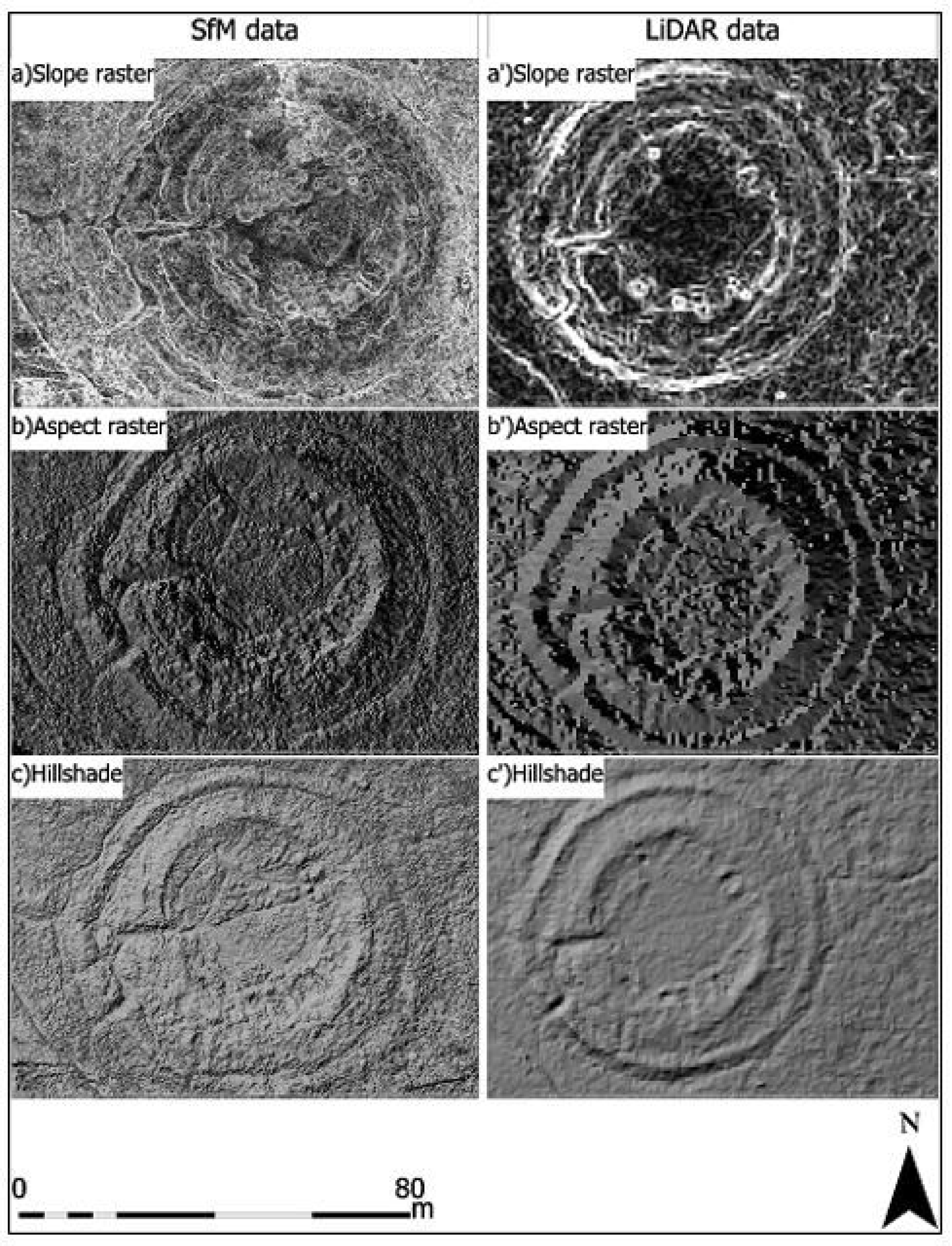
In addition, there are several visualization methods, such as slope images and aspect images derived from digital models, which can be used towards a successful detection of archaeological features [1,11,14,15,16]. Specifically, slope images display the vertical variations in the elevation models derived from LiDAR DTMs, while aspect images show the directions of vertical variations in the study sites [20]. In [20], a mound, and a possibly new shell ring and another mound were discovered. Additionally, [6] used a hillshade visualization of LiDAR data with a point density of 1 point/m² and successfully provided topographic details of Barwhill (north of Gatehouse of Fleet in Scotland) and detected several archaeological remains, such as linear features that signify old water drainage and another feature that corresponds to the Roman road. However, features could not be extracted from hillshade images, in some cases, due to the influence of the illumination model, which creates distortions and therefore hide some archaeological features. 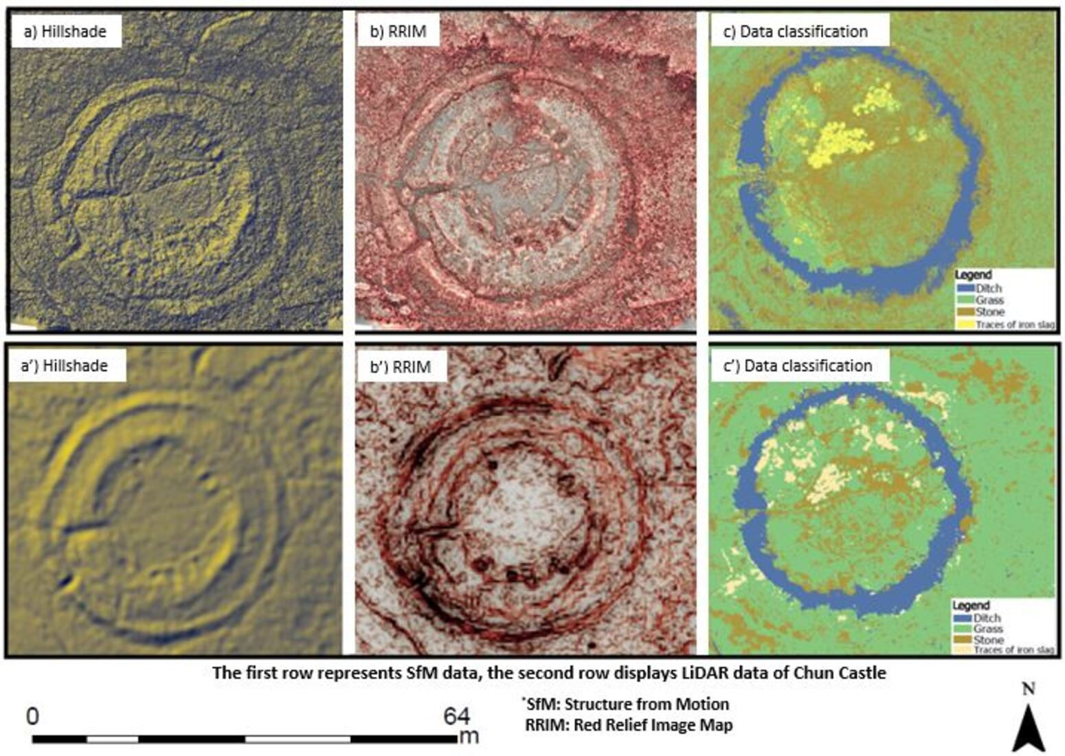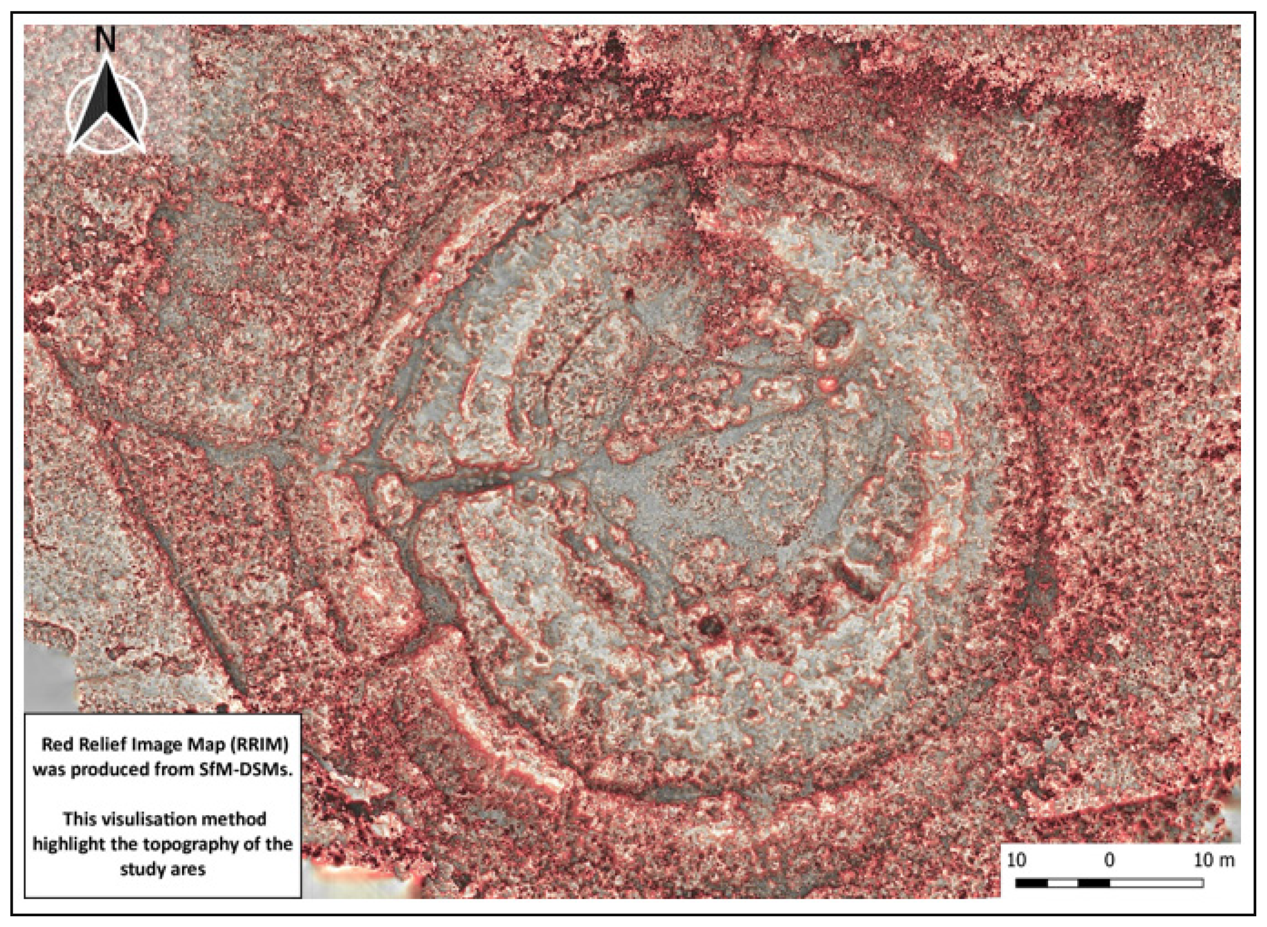Similarly, in [20], it was also found that the light in hillshade images could obscure topographies, so they created Red Relief Image Maps (RRIMs) to detect and digitize mounds using LiDAR data. RRIM is another visualization method and is suitable to represent and interpret monuments on various terrains, such as land surface, seafloor, and features on celestial bodies [14]. RRIM has overcome the limitations (e.g., light direction dependence, filtering, and a weakness for scaling) of other visualization methods, such as hillshade. In [15], different visualization methods were applied and evaluated under various conditions and they found that the RRIM technique brings relatively a great visualization advantage to the end user when compared to other methods, as it can successfully reveal subtle archaeological remains raster. Moreover, different visualizations techniques (e.g., hillshade, slope, positive openness) can be computed using the Relief Visualization Toolbox (RVT) for discovery and recognition of small-scale features [16,21].

Many studies have employed RS technologies in the discipline of archaeology and cultural heritage. Some focused on the discovery and recording of ancient features/sites for the first time [7,15,17]; others highlighted known archaeological features [6,11,13]. These studies are related to some extent to our research although some are particularly targeting larger areas (e.g., discovering new sites). Thus, UAV-based photogrammetry and LiDAR have the possibility to make substantial further contributions to archaeological management outcomes, and these methods provide secure detection and adequate characterization of the archaeological records. The aim of this study is to demonstrate a workflow for identifying and recording archaeological features using fine-scale RS approaches (i.e., Structure from Motion- Multi View Stereo (SfM-MVS) photogrammetry with drone data and LiDAR data) and make critical comparisons of their capabilities to identify archaeological features (possible remains). Aerial images and LiDAR data processing, classification tools, and visualization methods are utilized to detect and digitize potential archaeological features, including those hard to observe from ground-level but relatively easy to distinguish from above.

2. Materials and Methods

2.1. Study Area

Chun Castle (Figure 1) is an iron age hillfort near Penzance, in West Penwith, Cornwall, UK (50.1486° N, 5.6336° W) at 215 m above Ordnance Datum Newlyn (ODN) [22,23], built roughly 2500 years ago [23]. It contains several archaeological features (e.g., stones, walls, and potteries), which are about 2000 years old [3,24]. The castle has a nearly circular construction, ringed by two stone walls, with a ditch in front of each wall. Excavation works in 1930 and 1926 were implemented to explore the castle [3,4]. The latter studies revealed traces of oblong huts and an inner courtyard belonging to the Iron Age, but these huts apparently no longer exist. In 1930, several fragments of pottery (demonstrating a medium roughness with a mixture of quartz) were also found, which are 0.03 m diameter and 0.01 m thickness [4]. Additionally, a furnace for mineral processing constructed over round structures in the Area of Interest (AOI) was identified. Presumably, the site was originally a place for ceremonies and local tribes [25]. Later, in the 16th century, the furnace was built for smelting and production of minerals and tin inside the fort [26,27]. The castle was then pillaged in the 18th century for stone to build houses and pave roads in Penzance [22,23]. The archaeological features already identified in the previous literature are summarized in

Table 1. Archaeological features from previous studies revealed in the study site using excavation methods.

Features Identified	Reference
Potential buildings	[3,4,23]
Pottery, flint, and glass	[3,23]
Furnaces	[3]
A castle well	[23]
Hearths accompanied by quantities of charcoal.	[3]
Hammer-stones	[3]

.

2.2. Remote Sensing Data

Two RS datasets are evaluated in this study to determine which dataset performs most effectively for the detection of supporting archaeological monuments: (i) DSMs derived from raw topographic LiDAR data and (ii) DSMs generated from SfM photogrammetry.

2.2.1. LiDAR Dataset

Raw topographic LiDAR data were captured during July and August 2013 using an Optech ALTM 3100 EA laser scanner for the Tellus South West project (www.tellusgb.ac.uk). The Applanix Global Positioning System (GPS) was used to create 74 random ground control points (GCPs) distributed in Cornwall and Devon to georeference the LiDAR survey product [28]. The spatial reference of the LiDAR data is OSGB 1936/British National Grid (EPSG: 27700). Calibrated LiDAR point clouds were processed into DSMs by Geomatics (Environment Agency) applying Terrascan software [28]. LiDAR DSMs are used in this study since the raw data of the study site are not available. LiDAR DSMs are obtained from the UK Centre for Ecology and Hydrology project in the Southwest (https://www.ceh.ac.uk) and downloaded from (https://catalogue.ceh.ac.uk/documents/b81071f2-85b3-4e31-8506-cabe899f989a) at a spatial resolution of 1 m with average accuracy of 0.25 m [29]. This resolution is sufficient in this research because there is not much more information that could be extracted from the LiDAR raw data that are smaller than 1 m topographic resolution. There is still a possibility to grid the raw data (in case of availability) at a higher resolution (e.g., 0.5 m), but in this case, a gap-filling algorithm would be the only choice to implement this option. Further, the available point density sets a limit to the amount of information that could be extracted from these data. Therefore; increasing the spatial resolution of this particular dataset would potentially not provide any additional useful information. This dataset was also used in other studies [30,31,32] and delivered interesting findings. Moreover, Refs. [6,20] used LiDAR data with the point density of 1 point/m² and they successfully detected several archaeological remains of AOIs. In addition to the LiDAR data, a second DSMs dataset was created from raw UAV-images using the SfM method at a spatial resolution of 0.04 m.

2.2.2. Photogrammetric Dataset

Data Collection

Data collection of the photogrammetric dataset took place at Chun Castle on 6 June 2019. Before carrying out the aerial survey, GCPs survey were carried out using the RTK- differential Leica GS08 system. A total of 15 ‘iron-cross’ markers were surveyed across the study site as GCPs and positioned spatially applying differential GNSS. The iron-cross markers were distributed in the AOI to ensure the position of the GCPs around the boundaries of the study site and nearby the castle center [33]. The markers should be free from grass/vegetation that might obstruct a clear view from the air. A local reference station was measured using a two-hour static DGPS observation period; after post processing, the spatial accuracy of the local reference station was 0.02 m horizontally and 0.05 m vertically. Then, 15 GCPs were deployed and geolocated in the AOI relatively. These points were used later to re-align point clouds for georeferencing the aerial survey data.

The objective of the UAV survey is to acquire a photogrammetric data set to generate an orthomosaic map and DSMs for Chun Castle. We used a DJI Mavic 2 Pro Drone (https://www.dji.com/uk/mavic-2), equipped with a Hasselblad digital camera (5472 × 3648 pixels), which has a rolling electronic shutter (

Table A1. Specifications of the Hasselblad UAV digital camera used in this study.

Category	Specification
Aperture	f/2.8
Electronic Shutter	1/8000s
Image size	5472 × 3648 px
Effective Pixels	20 million
FOV	Roughly 77°

in Appendix A). This platform weighs ca. 907 g and costs less than £1,500. In this study, the flights were performed within a visual line of sight at an altitude of 80 m over the AOI with a 6.9 cm/px Ground Sampling Distance (GSD). This altitude (80 m) was chosen, as the flight height directly influences achievable GSD and consequently, effects the details that could be identified from the UAV imagery [34,35,36]. There are several studies (e.g., [35,36,37]) with flight altitude greater than 80 m that received fine-grain maps of the AOIs. This altitude was selected to obtain sufficient GSD that enable us to interpret and detect the topographic features of the archaeological site (Section 3). The aerial images in this work were captured by keeping the digital camera at fixed focal length of 28 mm. The minimum overlap and sidelap was specified to be 80%, and the shutter speed was 1/640th of a second, which was adequate to reduce motion blur and obtain more consistent extracted features [36,37]. The study site was surveyed with a programmed flight using open-source Mission Planner software (http://planner.ardupilot.com/); this software is used as a dynamic control supplement to set up flight missions and monitor the drone status while in operation. Drone flights were conducted within a few hours of solar noon (e.g., 13:00) in the sense that the brightness conditions are likely to impact the photogrammetric reconstructions [34,35,36]. The platform was flown for 15 minutes over the study site to capture 161 aerial images; the flight details are summarized in

Table 2. Unmanned Aerial Vehicle (UAV) flight parameters used in the photogrammetric data collection campaign.

Parameter	Setting
Flying height	80 m
Focal length	28 mm
Overlap and sidelap	80%
Camera ISO	200
Margin	15 m
Exposure value (Ev.)	−0.7
Shutter speed	1/640th s

.

Orthomosaic and DSM Generation

Following data capturing of the UAV images, SfM photogrammetry pre-processing phase was implemented. Several computer programs are available for SfM photogrammetric processing, such as Pix4Dmapper, Recap, and Metashape. Agisoft Metashape Professional software (v.1.5) (https://www.agisoft.com/) was used in this study since it is efficient and effective in the production of, to some extent, accurate dense point clouds from aerial images comparing with other photogrammetry software [33,34]. The workflow begins with photo alignment that applies SfM methods to seek common points on aerial images, match them, and run point clouds triangulation [36,38]. The bundle block adjustment algorithm is then implemented to refine the camera position for individual aerial images and enhance the 3D reconstructions [33,34,35]. The resulting sparse point cloud is applied to create a 3D mesh of the site/ scene. Next, ground control markers used to georeference the models. Specifically, 15 markers were placed in Agisoft Metashape. Then, GCPs were imported and manually recognized within the aerial images to ensure geolocation with the spatial positions of the individual photos. Multi-view stereopsis techniques were then applied to create dense point clouds based on adjusted camera positions, GCPs, and RGB aerial images [39]. Roughly 12 million (12,057,994) points are generated from this initial processing step in this 3D dataset. The outputs of the aerial images pre-processing phase are a textured mesh, an orthomosaic map, and DSMs. These outputs were analyzed in ArcGIS Pro (v.2.4) (https://www.esri.com) to identify any possible archaeological features.

2.3. Visualization Methods

The first step in post-processing phase was to create four visualization raster images from each model (i.e., LiDAR DSM and SfM-DSM). Visualization methods could provide an essential contribution to detect topographic information acquired by RS approaches e.g., LiDAR [2,14]. Combining and overlaying visualization raster data in GIS are considered a key component in interpretation and interaction with the simulated environment [40,41]. These visualization raster images are: Slope image, aspect image, shaded relief map (hillshade), and RRIM.

2.3.1. Slope and Aspect Raster

Slope raster focuses on altitude changes in the landscape. Most GIS packages apply a 3 by 3 neighborhood for several raster operations (e.g., slope and aspect) [42,43]. The slope is usually calculated in degree units using the original DSMs as inputs, see Equation (3). For more clarification,

Table 3. 3 × 3 window cells in a raster image.

a	b	c
d	e	f
g	h	i

represents the values of the cell (e) and its eight neighbors (from a to i) to define both horizontal and vertical deltas [42]. The slope raster image can identify the steepness of individual cells in the raster image; where each pixel is colored based on the terrain slope [20]. However, the aspect image colors the pixels according to the slope orientation [11]. The merit of using the aspect raster in this study, in addition to the orthomosaic image, lies in the possibility of identifying the features that have already been identified by previous studies within the study site (e.g., the entrance, ditches).

2.3.2. Hillshade Raster

The hillshade raster is a shaded-relief image that highlights landscape elevation changes [2,30]. The illumination parameters (Azimuth: 315, altitude: 45, and Z-factor: 1) are simulated in this study to create the shaded-relief image. The azimuth and altitude specify the relative position of the sun to generate the 3D models (shaded-relief). The azimuth is representing the relative location of the sun along the horizon, which is measured clockwise from the north (0/360 degree), east, south, and to the west (270 degrees). However, the altitude parameter refers to the elevation angle of the sun over the horizon ranging between 0 (the elevation angle on the horizontal plane of the reference frame that results in creating 3D models with minimum illumination) and 90 degrees (overhead the horizontal plane that results in creating 3D models with maximum illumination). Z factor modifies the measure of the elevation units (Z) when varies from the horizontal units (X and Y) of the input raster. In this case, the horizontal and vertical units are all in the same unit (meter), therefore the Z factor was set to 1. The utility of this visualization method is that it helps the user understand and comprehend the topographic details [1,14]. Nonetheless, one of the weaknesses that could be encountered in hillshade image is that the illumination could cause deformations that lead to obscuring specific terrain features [14,42]. To avoid this, RRIMs (known as shade-free relief maps) are applied to obtain clear topographic features of the AOI since they compare favorably with other visualization methods [42,44].

2.3.3. Red-Relief Image Mapping (RRIM)

RRIM is a visualization method based on multi-layered topographic data (i.e., positive openness, negative openness, and topographic slope) that is computed from DSMs [14]. Openness is an angular measure of the relation between horizontal distance and surface relief, it represents the enclosure (negative) and dominance (positive) of a landscape position, and is applied to visualize topographic details [44]. Positive openness signifies the convexity of landscapes, such as ridge and crest, while negative openness signifies the concavity of landscapes, such as valley and gully [15,42]. Certain parameters, such as radial limit and number of sectors, were selected to create topographic openness. The radial limit depends on the landscape features, cell size, and grid size. In this research, a variety of radial limits (2 m, 10 m, 30 m, and 50 m) are tested to identify the most appropriate value to use for calculating the deferential openness raster; 10 m radial limits were selected, as this provides a relatively more detailed raster image for Chun Castle. The number of sectors was configured at 8, which is the standard value used to specify the number of azimuths [44]. There are two available methods to implement the openness calculations: The sector method and the multi-scale method. One of the main drawbacks of the multi-scale method is that it generates pyramid layers, which deliver less accurate openness parameters than those that could delivered from sector method [44]. For this reason, the sector method was employed in this research to implement the openness calculation. To extract RRIMs, a differential openness raster (I) was applied to calculate openness parameters following Equation (1), where I is the differential openness raster, O_p is the assessment of the positive openness (which computes topographic concavity), and O_n is the assessment of the negative openness (which estimates topographic convexity) [14,15].

$$\mathrm{I}=\frac{\left(\mathrm{Op}-\mathrm{On}\right)}{2}$$

(1)

The RRIM is a shade-free method that effectively represents fine structure of 3D topographic data. This method provides the possibility to visualize relatively higher-resolution 3D raster images than obtained with other visualization methods (e.g., hillshade). Hence, it suitable for wide range of topographic data, such as LiDAR and photogrammetry [11,14]. Therefore, RRIMs are generated in this study by overlapping the differential openness raster with the slope raster. RRIM values are then used to generate a combined map that illustrates convexities, and concavities with the topographic slope raster in red color [20,44], see

Table 4. The layers (slope maps, differential openness, and topographic openness) used to create the Red Relief Image Maps (RRIMs).

Layer	Setting While Creating the Layer
Topographic openness	Radial limit	10 m
	Method	Sectors
	No. of sector	8
Differential openness	Resampling	Bilinear
	Brightness	50%
Slope raster	Output Meas	Degree
	Brightness	80%

.

2.4. Classification Algorithms

2.4.1. Supervised and Unsupervised Classification

In this work, some archaeological features are identified manually while other features are detected automatically. The use of aerial images and mosaics has been rooted in manual interpretation where the user should visually seek to identify objects of interest [20]. Such manual analysis is a productive approach for feature detection, although it is likely to limit the potential and efficiency of RS techniques over larger areas (e.g., <1 ha). In this research, the manual detecting and digitizing of archaeological features is based on visualization methods. Automated feature digitizing methods have not replaced manual extraction methods since manual extractions still have the flexibility and adaptability to apply to various types of data. Specifically, monuments are identified manually from the visualization raster images in combination with the orthomosaic image where pixels are found to be roughly similar in spectral aspects. The identified archaeological objects are digitized as polygons (e.g., the castle well) and polylines (e.g., the entrance) using ArcGIS Pro software (v.2.4) (https://www.esri.com).

In addition to the manual approach, automatic classification methods are applied such as ISO cluster tools and supervised classification, which consider essential tools for extracting archaeological information from RS data [12]. These classification methods specify land classes to pixels and are likely to increase productivity by minimizing time-consuming manual feature extraction [45,46]. Generally, ISO classification is where objects or areas are assigned to classes depending on the raster image analysis without selecting pre-defined sample classes [11,12,47]. The users can set the algorithm to group pixels into classes and specify the required number of classes to assign objects. In supervised classification, users can specify sample pixels in a raster image to generate certain classes and use as reference classes in order to classify all pixels in the raster [46,48]. ISO cluster and supervised classification tools are used in several archaeological studies (such as [12,15,48]) for the identification of archaeological features. Unsupervised classification tools were also applied in this archaeological application due to various reasons: Classes do not have to be specified beforehand, unrecognized classes might be revealed, and generally, it requires a minimum quantity of inputs in contrast with supervised classification.

Despite the beneficial outputs that could obtain from the ISO Cluster method, in this research, supervised classifications were used to develop final outcomes analysis. A range of algorithms in the supervised classification are available; for instance, Support Vector Machines (SVM), Maximum Likelihood (ML), and Neural Networks (NN). ML is the standard parametric algorithm and presumes data for each class in a raster are normally distributed [49,50]. NN algorithm use convolutional layers to classify a raster that improves labelling procedure, where landscape data could be extracted at various levels (e.g., object level, pixel level, and patch level) [19]. These algorithms can be applied using various software packages, such as Erdas Imagine, Google Earth engine, and ArcGIS to achieve automatic land extraction. Specifying training data is to some extent more important than the choice of a certain classification method to acquire relatively higher classification accuracy of the classified raster images [51]. However, several studies (e.g., [49,52,53]) found that SVM performs better if compared to other classifiers (e.g., ML algorithm) and is likely to reduce the classification errors of the land cover information. Therefore, the SVM algorithm was used in this work to extract the archaeological features from RS data in ArcGIS Pro. More specifically, in the supervised classification, the SVM classifier was trained to assign pixels to four different classes (ditch, stones, Iron slag, and grass) using training samples. The training data are created for individual class category by drawing polygons around objects in the raster images (i.e., orthomosaic image) using the training samples manager tool. This was applied to provide data about the size and number of samples and also to enhance the overall accuracy of the classification process. Nonetheless, classified outputs produced by the SVM algorithm can contain certain random noise. To improve classification results, a post-classification method was carried out. Specifically, various algorithms are available to eliminate noise and change misclassified pixels to the correct class. In this study, the re-classifier tool from ArcGIS Pro was applied to make edits to particular objects/ features and address the errors of the classified outputs.

2.4.2. Data Validation

Accuracy assessment tools were employed to estimate and assess the accuracy (i.e., the degree of correctness) of the classified results. This technique is important for assessing the data derived from RS resources and is considered a critical component for a range of studies including archaeological research projects [15,18,19,54]. The most accurate assessment was derived from the errors/ confusion matrix validation assessment to describe the accuracy of the applied classification process [55,56,57,58,59]. This matrix is used for full reporting of overall accuracy, user’s accuracy, producer’s accuracy, and Kappa [47,59]. Using geoprocessing tools, a stratified random sampling approach is applied based on the classified map to create a set of points (500 points) to guarantee all the classes are adequately characterized. Then, these assessed points are validated using Google Earth imagery (reference data) to assign individual points to their individual real classes (Figure 2). These points are then assembled into tables to contrast the real class for individual points with their classification raster. With the confusion matrix method, accuracy and kappa values are represented from 0 to 1, where 1 indicating 100% accuracy percentage [58,60]. Kappa calculates the agreement between the truth values and the classified values. The following Equations and

Table 5. The GIS Pro confusion matrix; rows represent predicted classes, while columns represent actual classes.

		Classes from Reference Source
		A	B	C	D	Σ
Classes from classified source raster	A	AA	AB	AC	AD	ΣA
	B	B-A	BB	BC	BD	ΣB
	C	CA	CB	CC	CD	ΣC
	D	DA	DB	DC	DD	ΣD
	Σ	ΣA’	ΣB’	ΣC’	ΣD’	N

showing how the validation process is implemented in this research [54,57]. Thus, an interpretation approach of SfM-MVS photogrammetric and LiDAR data was presented using visualization methods and automatic classification approaches to detect archaeological features in Chun Castle study site and shed light on archaeological findings that belong to the Iron Age and the later Roman period.

$$\mathrm{Total}\mathrm{accuray}=\frac{{\sum }_{\mathrm{i}=1}^{\mathrm{r}}\mathrm{Xii}}{\mathrm{N}}\ast 100$$

(2)

$$\mathrm{User}’\mathrm{s}\mathrm{accuracy}=\frac{\mathrm{Yii}}{\mathsf{\Sigma }\mathrm{x}\mathrm{i}’}\ast 100$$

(3)

$$\mathrm{Produces}’\mathrm{s}\mathrm{accuracy}=\frac{\mathrm{Yii}}{\mathsf{\Sigma }\mathrm{xi}}\ast 100$$

(4)

$$\mathrm{Kappa}\mathrm{coefficient}=\frac{\mathrm{N}{\sum }_{\mathrm{i}=1}^{\mathrm{r}}\mathrm{Xii}-{\sum }_{\mathrm{i}=1}^{\mathrm{r}}\left(\mathrm{xi}\ast \mathrm{xi}’\right)}{{\mathrm{N}}^2-{\sum }_{1=1}^{\mathrm{n}}\left(\mathrm{xi}\ast \mathrm{xi}’\right)}$$

(5)

where Y_ii is the value that has been classified correctly belonging to class (i), N is the sum of classified (predicted) data compared to actual data, x_i is the sum of classified data belonging to individual classes (class i), x_i’ is the sum of actual data belonging to individual classes (class i), and X_ii is the diagonals numbers that have been classified correctly according to the actual data.

3. Results

3.1. Interpretation Analysis Results

Point-clouds derived by applying SfM-MVS drone-based image processing created realistic 3D model representation of the Chun Castle (Figure 3). Later, when visual raster images were produced and interpreted, it was found that the slope raster reveals the border of the entrance and emphasizes the outline of the archaeological features as compared to the original DSM. However, the hillshade raster provides a clearer outline of the area used for mineral processing display (Figure 4). The topographic features of the study site are also identified through the RRIMs. The RRIMs in this study provides less distorted and clearer views than other raster images (slope, aspect, and hillshade raster images) and identified the topographic features (e.g., castle entrance, ditch, circular and leaner monuments). These outcomes deliver the crucial information and visualization potentials to interpret the identified features (Figure 5). Based on these visual rasters, and the orthomosaic image derived from the MVS-SfM data, the following archaeological features have been visually interpreted: A possible area for mineral processing (163.63 m²), ditches (external: 5562.51 m²; internal: 3783.63 m²), a linear feature (A: 34.21 m), and three circular shapes (I’: 2.28 m²; II: 5.41 m²; III: 1.56 m²). Furthermore, six possible remains of constructions (i.e., possible circular houses or traces of chambers), which are formed of walls made of stone posts, are also digitized in this study. The size of these linear traces is: [Chamber (I) 11.74 m; Chamber (II) 20.31 m; Chamber (III) 9.49 m; Chamber (IV) 6.35 m; Chamber (V) 5.59 m; Chamber (VI) 10.87 m]. The size of these archaeological features is relative to the spatial resolution of the data (Figure 6).

In addition to the SfM data, LiDAR-DSMs are also investigated and visually interpreted. Archaeological monuments are identified (e.g., boundaries, ditch, and the castle entrance) based on the visual raster images produced from LiDAR dataset (Figure 6 and

Table 6. The areas of the archaeological features detected in this work using SfM and LiDAR data analysis.

Feature	SfM Data	Area (m2)	LiDAR	Area (m2)
Circular shape I	✓	2.28	✓	3.50
Circular shape II	✓	5.41	✓	5.97
Castle well (III)	✓	1.56	✓	2.46
Circular shape (IV)	n/a	n/a	✓	4.06
Circular shape (V)	n/a	n/a	✓	5.06
External ditch	✓	5562.51	✓	5524.21
Internal ditch	✓	3783.63	✓	3747.06
Field for mineral processing	✓	153.47	✓	145.32

and

Table 7. The lengths of the archaeological features identified in this study using SfM and LiDAR data analysis.

ID	Feature	SfM Data	Length (m)	LiDAR	Length (m)
A	Polyline I	n/a	34.21	✓	38.74
B	Polyline II	n/a	n/a	✓	56.64
C	Polyline III	n/a	n/a	✓	33.33
D	Chamber I	✓	11.74	n/a	n/a
E	Chamber II	✓	20.31	n/a	n/a
F	Chamber III	✓	9.49	n/a	n/a
G	Chamber IV	✓	6.35	n/a	n/a
H	Chamber V	✓	5.59	n/a	n/a
I	Chamber VI	✓	10.87	n/a	n/a

). These monuments are: Ditches [external: 5524.21 m²; internal: 3747.06 m²], linear monuments [Polyline (I) 38.47 m; polyline (II) 56.64 m; polyline (III) 33.33 m] and six circular shapes [Circular shape (I) 3.50 m²; circular shape (II) 5.97 m^2, circular shape (III) 2.46 m², circular shape (IV) 4.06 m², circular shape (V) 5.06 m²]. To our knowledge, these archaeological features were first detected and digitized using RS approaches (Table 6, Table 7, and

Table A2. A summary of the archaeological features detected in this study after implementing visualization methods, ISODATA clustering algorithm, and SVM classification using LiDAR and SfM datasets.

Feature	SfM Data	LiDAR
Castle entrance	Manual & Automated	Manual & Automated
Circular houses	Manual	n/a
External ditch	Manual & Automated	Manual & Automated
Internal ditch	Manual & Automated	Manual & Automated
Castle well	Manual	Manual
Circular shapes	Manual	Manual
Area for mineral processing	Manual & Automated	Manual & Automated
Unknown features	Manual	Manual

in Appendix A).

In addition to the manual detection analysis, automatic detection tools were applied (i.e., ISODATA algorithm) to create an unsupervised classification and supervised classification analysis to identify archaeological features. The results from supervised classifications (Figure 7) were similar to those achieved from the ISO Cluster method (Figure A2 in Appendix A). The random stones inside the castle are detected and mapped automatically after interpretation-based Visualization methods. Some of these stones are possible remains of huts that were built between the Iron Age and the Roman period. Additionally, the castle ditch and a triangular shape (the field for mineral processing) are also detected and digitized automatically in this study. There is a section inside the fort still containing traces of iron slag and tin; hence this part was automatically detected and digitized by applying classification algorithms. Thus, ditches, the mineral field, random stones, traces of iron slag, and grass were automatically digitized by employing these approaches.

3.2. Validation Results

In this research, the outcomes of the classification results are validated based on the confusion matrix analysis. The results delivered from applying the validation analysis (Figure 8) show that the validation results of SfM data are relatively more accurate than results produced from the LiDAR datasets, although the same supervised algorithm (i.e., SVM) was applied and the same number of targeted classes was used for both LiDAR- and photogrammetric-derived maps (classification maps) of the same landscape. Training samples are also one of the factors that impact the classification accuracy [53], as the total number of the training samples represent a certain class (e.g., stones); consequently, the location of these samples should be based on relatively high-resolution maps in order to obtain higher classification accuracy. This means that the validation results also correlate with the spatial resolution of the classification map [53]. Thereby, the overall supervised classification accuracy assessment benefits from higher spatial resolution maps. In this study, the spatial resolution of the photogrammetric dataset is higher than the LiDAR dataset, which explains the validation results (the user’s accuracy, producer accuracy, and kappa analysis) of the SfM data that are comparatively higher than those delivered from the topographic LiDAR data. Moreover, Kappa measurements of the classification maps derived from LiDAR and photogrammetry were 72.7% and 77.8%, respectively. Based on the user accuracy (

Table A3. ArcGIS Pro confusion matrix of the SVM classification map generated from LiDAR data.

ID	Class Value	C-10	C-40	C-50	C-70	Total	U-Accuracy	Kappa
1	C-10	20	1	0	1	22	0.909	0
2	C-40	7	202	6	27	242	0.835	0
3	C-50	0	3	11	1	15	0.733	0
4	C-70	0	32	0	189	221	0.855	0
5	Total	27	238	17	218	500	0	0
6	P-Accuracy	0.741	0.849	0.647	0.867	0	0.844	0
7	Kappa	0	0	0	0	0	0	0.728

and

Table A4. ArcGIS Pro confusion matrix of the SVM classification map generated from SfM data.

ID	Class Value	C-10	C-40	C-50	C-80	Total	U-Accuracy	Kappa
1	C-10	36	2	2	0	40	0.9	0
2	C-40	4	200	19	0	223	0.897	0
3	C-50	1	19	133	2	155	0.858	0
4	C-80	0	17	4	61	82	0.744	0
5	Total	41	238	158	63	500	0	0
6	P-Accuracy	0.878	0.840	0.842	0.968	0	0.86	0
7	Kappa	0	0	0	0	0	0	0.789

in Appendix A), ditches’ identification and digitization (external and internal) at the AOI from both datasets achieve the highest accuracy levels if compared to other features. Further, 90% of the identified features from the field being also detected and digitized in both photogrammetric and LiDAR datasets. Identifying stones obtained 73% and 85% coincidence between the mapped data, i.e., LiDAR and SfM methods, respectively, and ground data (reference data). Some of these stones are expected to be the remains of huts/houses dated to the Iron Age and Roman time period. Additionally, the SVM classification process successfully detected and mapped traces of iron slag. Even so, 85% and 74% of the mapped stones were confirmed to be identified from the SfM and LiDAR dataset correspondingly in a comparison with a reference map (Figure 2). The minimum accuracy delivered from the map classification analysis was 74.3% and 73.3% from SfM and LiDAR datasets, respectively. This assessment routine was also adopted in a previous [49] study.

4. Discussion

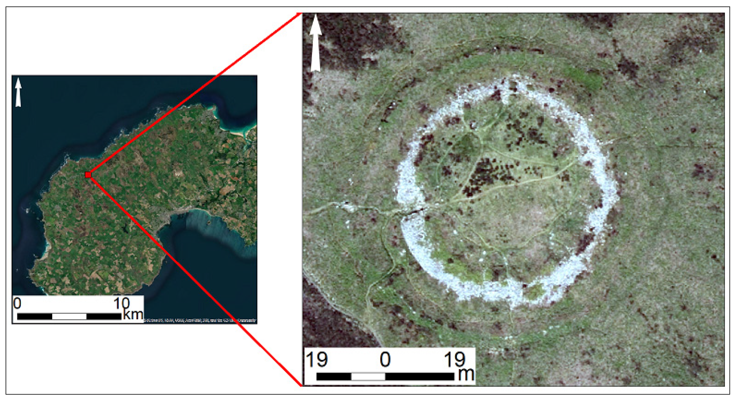
Studies by [3,4] were the first to identify archaeological monuments at Chun Castle, by implementing excavation methods. Work to date has concentrated on employing specific approaches for identifying archaeological landscapes (e.g., [10,11,18,20,59]) and has not yet focused on making critical comparisons of various non-invasive methods (i.e., RS) for detecting archaeological structures. This research demonstrates particular interpretation and analysis methods that were applied on products derived from two RS approaches (i.e., LiDAR and UAV-SfM datasets) and highlight the differences in their capabilities to detect new archaeological features (potential monuments) at the study site (Table 6 and Table 7).

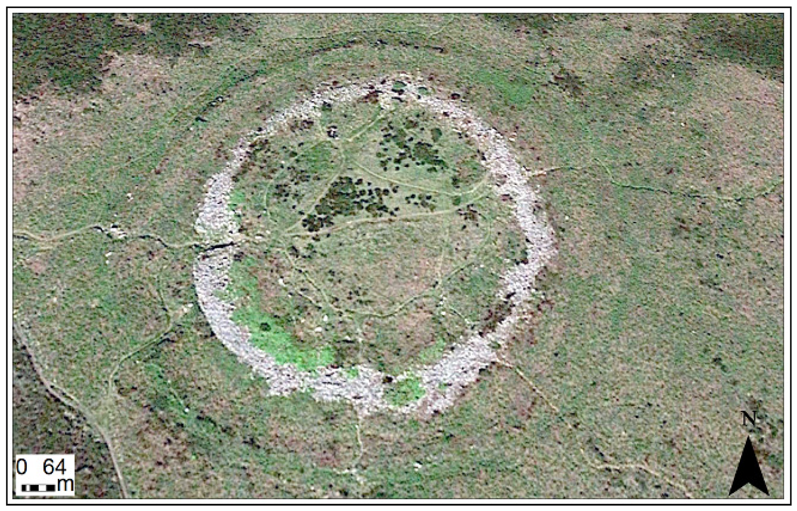
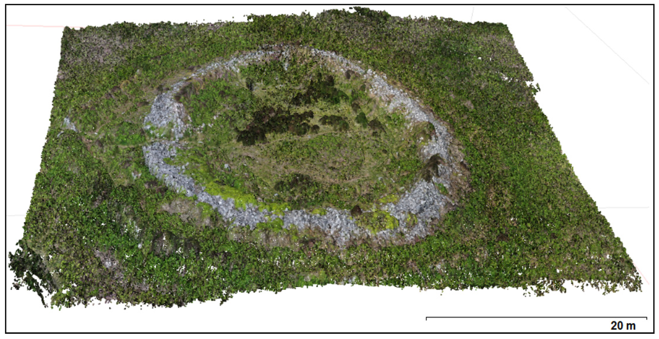
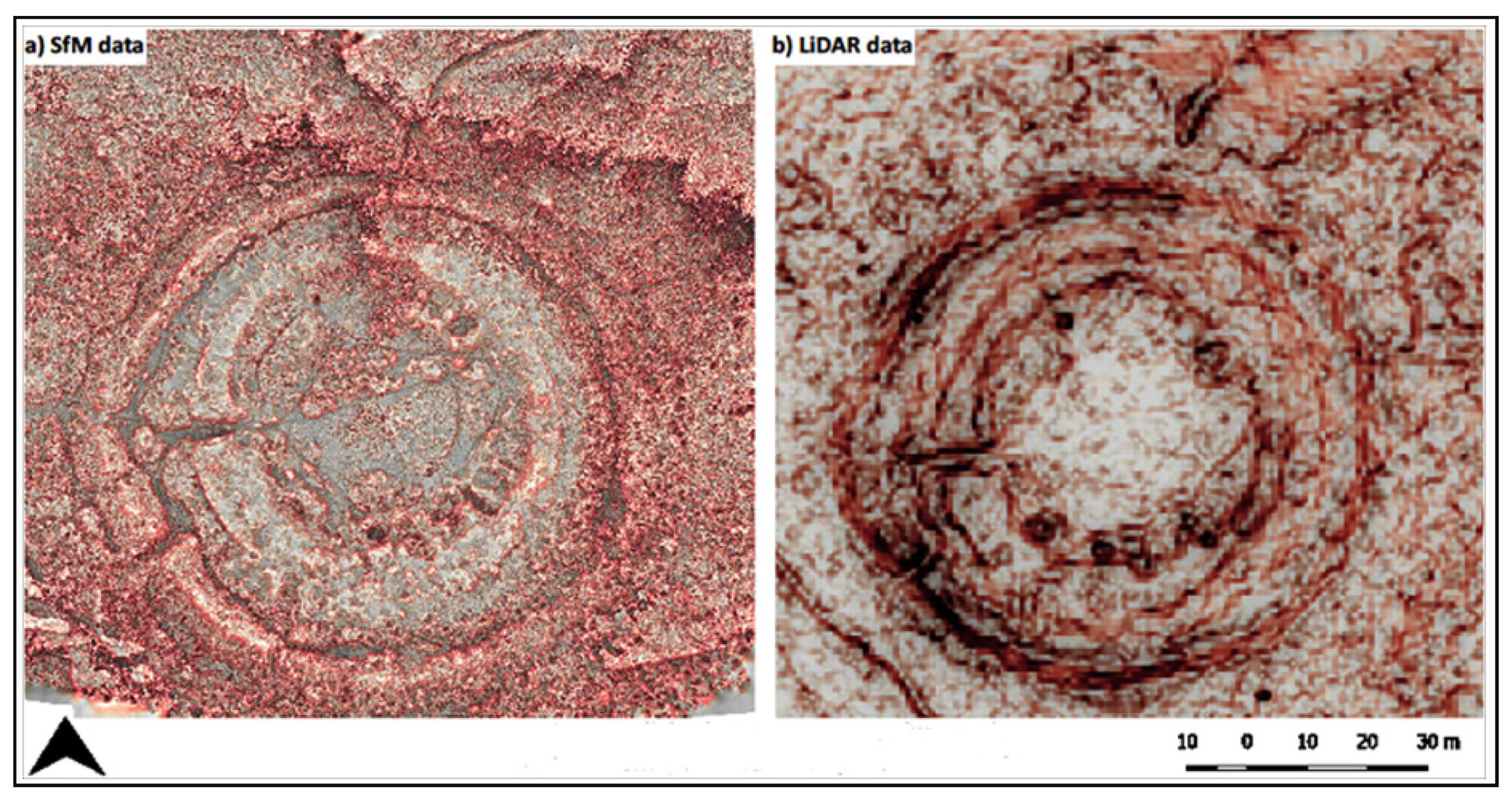
Chun Castle is in an extremely ruinous state. It was frequently challenging to identify archaeological objects from the RS data due to the number of loose stones covering the site. 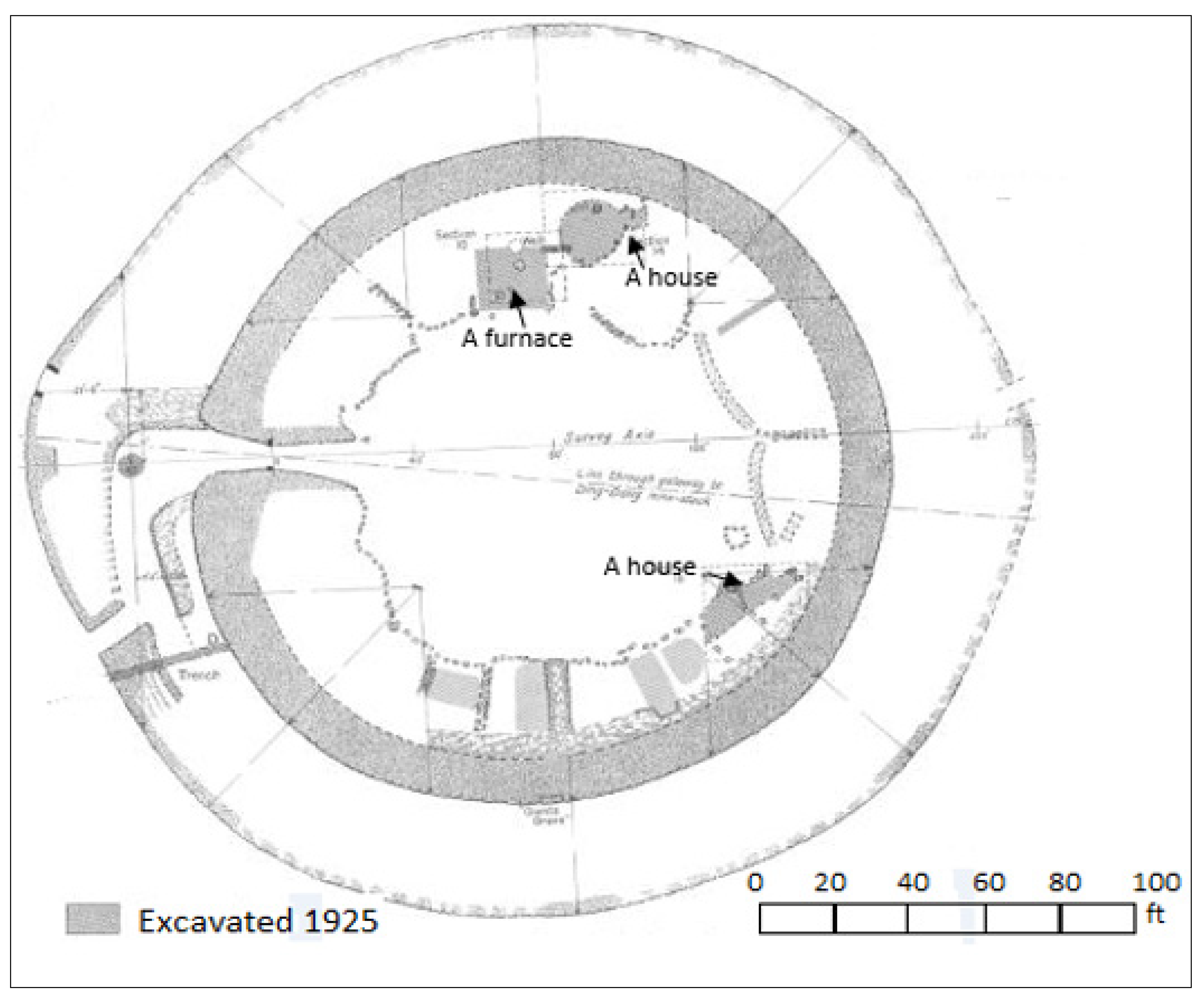In this study, various visualization methods are applied; the presented combination of the DSM, slope raster, and RRIMs delivered relatively more detailed, less distorted, and clearer raster images than other visualization methods (e.g., hillshade), allowing for the extraction of more information about the archaeological landscape (Figure 6). Using non- destructive methods, new findings are presented in this study site, which include possible traces of huts/houses, linear monuments, and circular structures. 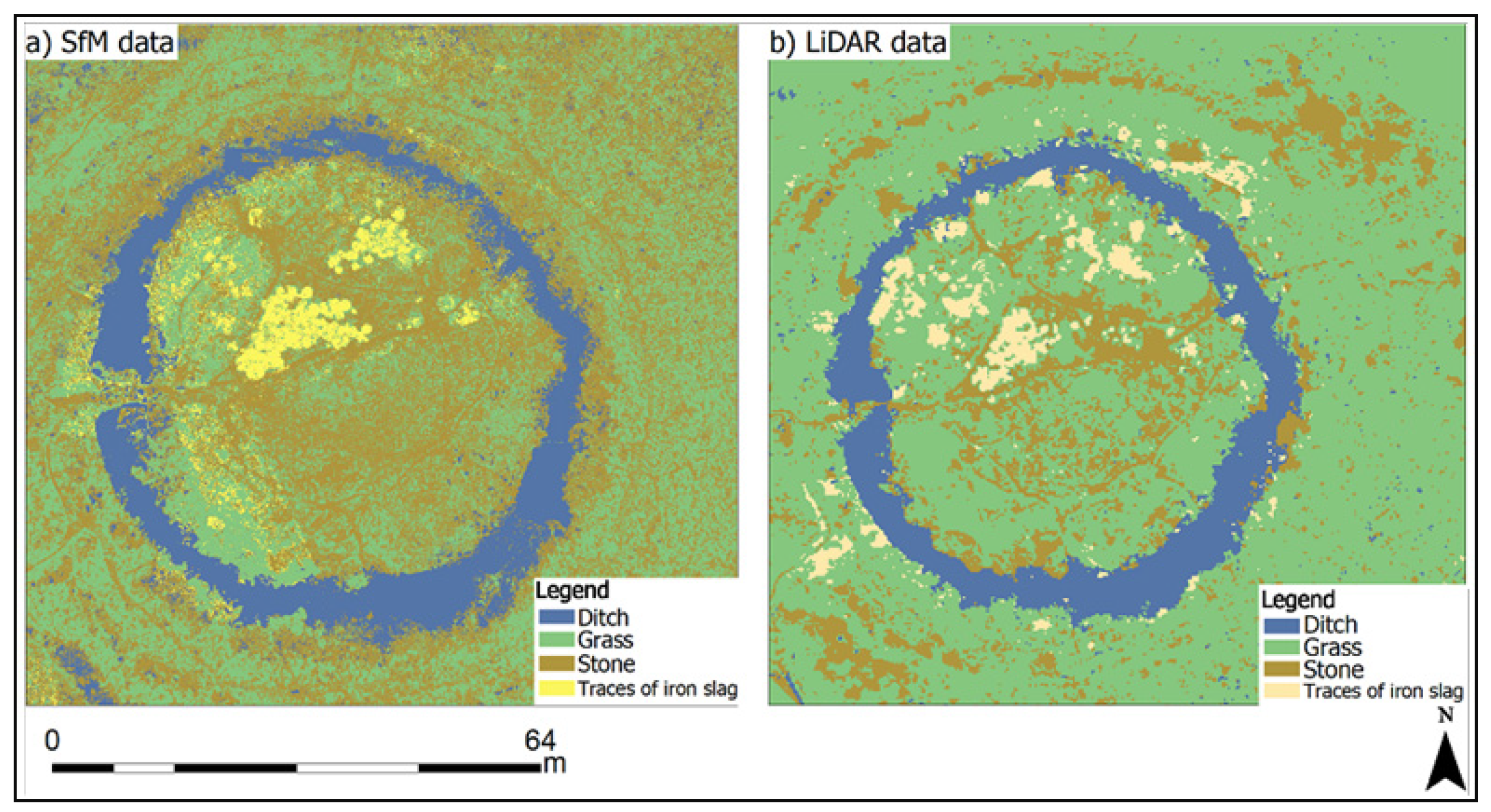In [27], possible archaeological remains were identified and interpreted, such as the castle well (one of the circular structures detected in this work), some pottery, huts, and a furnace by only utilizing excavation methods. A furnace in the fort (Figure 9), containing traces of iron slag and tin, indicates that the fort became a place for the blending, smelting, and production of minerals in the 16th century [3]. Additionally, and based on the excavation works by [4], there were huts in the inner courtyard belonging to the Iron Age, but that no longer exist. This might be due to the plundering that occurred in the 18th century to construct houses and pave roads in Penzance.

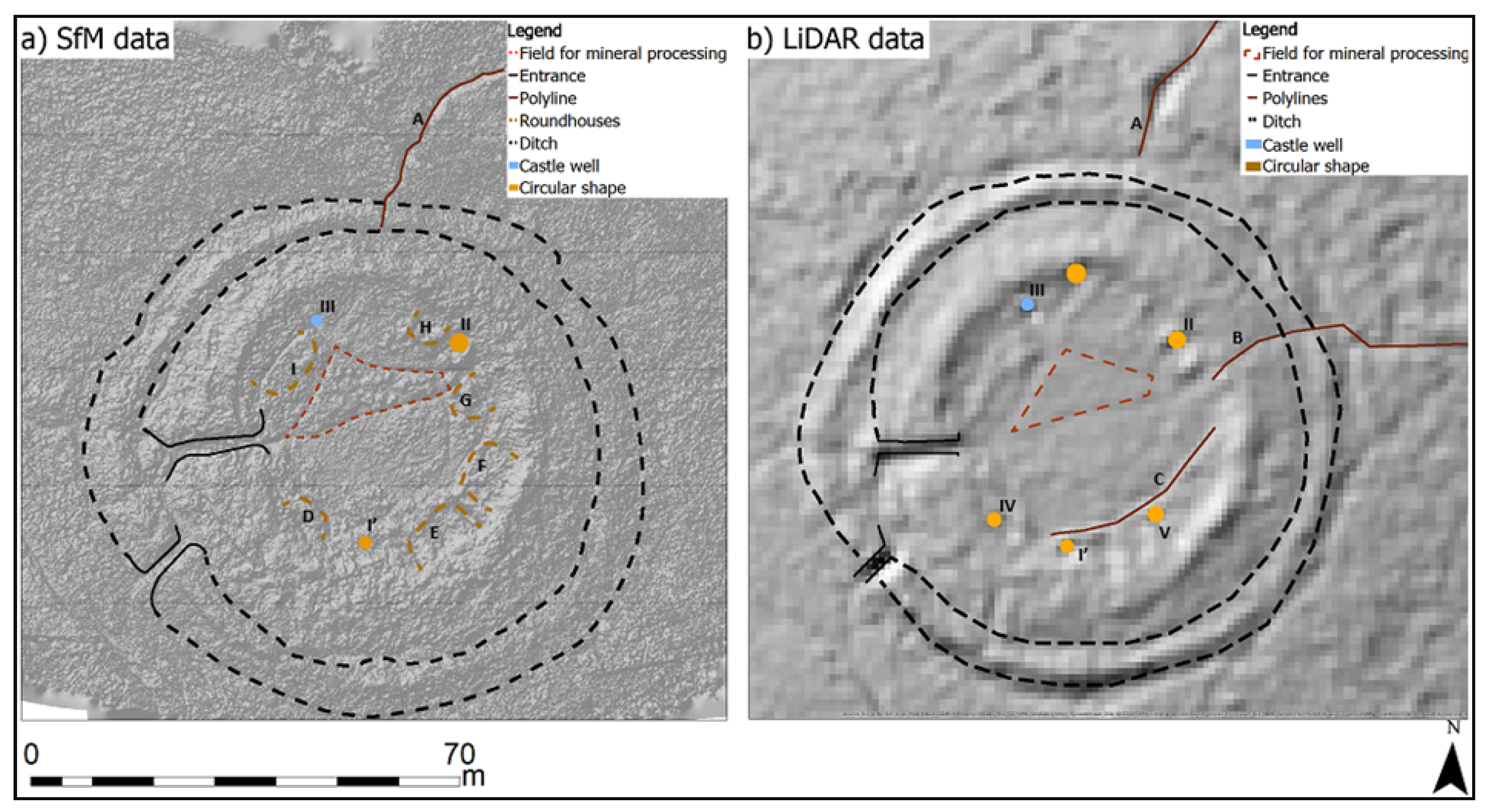
Further in this study, the RRIM and hillshade raster image derived from the SfM-DSMs shows some possible construction remains of round houses/chambers and these remains were interpreted and digitized (Figure 6 and Figure A1 in Appendix A). Circular huts, in general, are a normal form of Iron Age forts and have been revealed in most Iron Age castles [4]. Six ‘potential existence’ archaeological huts traces are found in this study; some of them have been revealed by previous literatures (Figure 9), as illustrated in Section 2. Furthermore, there was a castle well that had been used for providing water [27]. In general, wells are valuable elements in castles, and sometimes, castles had more than one well [61]. Cartwright [61] further states that around 80% of castles were supplied with one well and 20% had two or more wells. In this research, three circular features have been detected and one of these features was identified following its spatial positioning to be the castle well based on earlier identification in [3,27] studies.

In this work, archaeological features have been detected, quantified, and digitized at the fine-scale landscape from RS datasets. There are several features that were detected by SfM-MVS photogrammetry with UAV data but have not been identified by LiDAR (and vice versa), although the same processing and analysis methods were implemented in both datasets. This is due to the differences in spatial resolution between the two datasets. The reason is likely to be the spatial resolution of the SfM data, which is relatively higher than the resolution of the LiDAR DSMs for this particular site. In this study, the spatial resolution of the LiDAR data was 1 m, however there might be a possibility to grid the raw data (in case of availability) at a higher resolution (e.g., 0.5 m), which sets a limit to the amount of information extracted from this dataset. That means algorithms would be implemented by gap-filling the raw data; consequently, increasing the resolution in this particular case, would potentially not provide more useful information about the study site. Additionally, RS data were acquired on different dates, the LiDAR data were collected during July and August 2013 and the aerial photography in June 2019, the study site, to some extent, was not changed during that period (2013–2019). There are several factors that directly or indirectly affect topographic features and cause changes in a certain area, such as environmental damage (e.g., flood, earthquake, and fire) and human activities (e.g., vandalism, war, development, and excavation) [62]. The study site has not been exposed to these factors, nor any destructive tools, especially between 2013 and 2019 [61], so the archaeological area itself has not changed during that period. However, various archaeological features were likely to be obtained from both approaches due to the different settings and conditions (e.g., cameras, sensors, and resolution) of collecting each dataset. Accordingly, our understanding is promoted by this particular archaeological landscape that belongs to the Iron Age and the Roman period. The newly discovered possible huts and circular shapes in the castle helped to answer an archaeological question about how different methodological approaches (i.e., visualization methods and classification algorithms) can be applied for the detection of archaeological landscapes. Therefore, the merit of identifying archaeological structures here is to comprehend the capability of RS methods in interpreting and measuring structures/objects that might otherwise remain hidden.

5. Conclusions

In this paper, a non-destructive routine was presented to identify potential archaeological structures in Chun Castle site using LiDAR and UAV photogrammetry methods. The RS technologies allowed us to verify and understand the merits of the archaeological study site. Some features were identified and manually digitized based on the visualization methods (e.g., RRIMs) adopted. These methods resulted in a reliable identification of several potential hut monuments in the castle. ISO cluster and SVM classification algorithms were applied to automatically detect all archaeological objects in the site. The usage of various visualization approaches and classification tools in one archaeological site proved to be an adequate method for detecting hidden features. The algorithms that were adopted allowed for enhanced recognition of various suspected structures (e.g., roundhouse). The outcomes of the geospatial analysis allowed us to (1) detect and digitize newly archaeological objects, (2) map the shape of the fort, and (3) find unknown monuments (lines, circles) in the AOI. SfM photogrammetric data helped to detect hidden monuments in the archaeological landscape where LiDAR data provided relatively lower levels of detail. These differences were due to the various spatial resolution of the two datasets. The resulting DSMs and the produced visualization raster images, together with the utilized classification algorithms, allowed us to digitize the topographic features of the study site and detect possible monuments. Within this study, the possibilities of RS stand-alone methods (LiDAR and UAV-photogrammetry) in generating 3D models and identifying archaeological features of an ancient site are investigated. Our results concluded that the UAV-SfM and LiDAR are valuable data sources that could be applied in archaeological projects to improve potentials for new findings. For future work, we recommended the application of fusion RS approaches since there is a possibility to obtain relatively more information of the archaeological sites. Consequently, we conclude that applying fusion RS methods are likely to improve the interpretation performances of the RS source data and deliver relatively more archaeological data compared to the RS stand-alone approaches.