
Efficient and High Path Quality Autonomous Exploration and Trajectory Planning of UAV in an Unknown Environment

Abstract
:1. Introduction
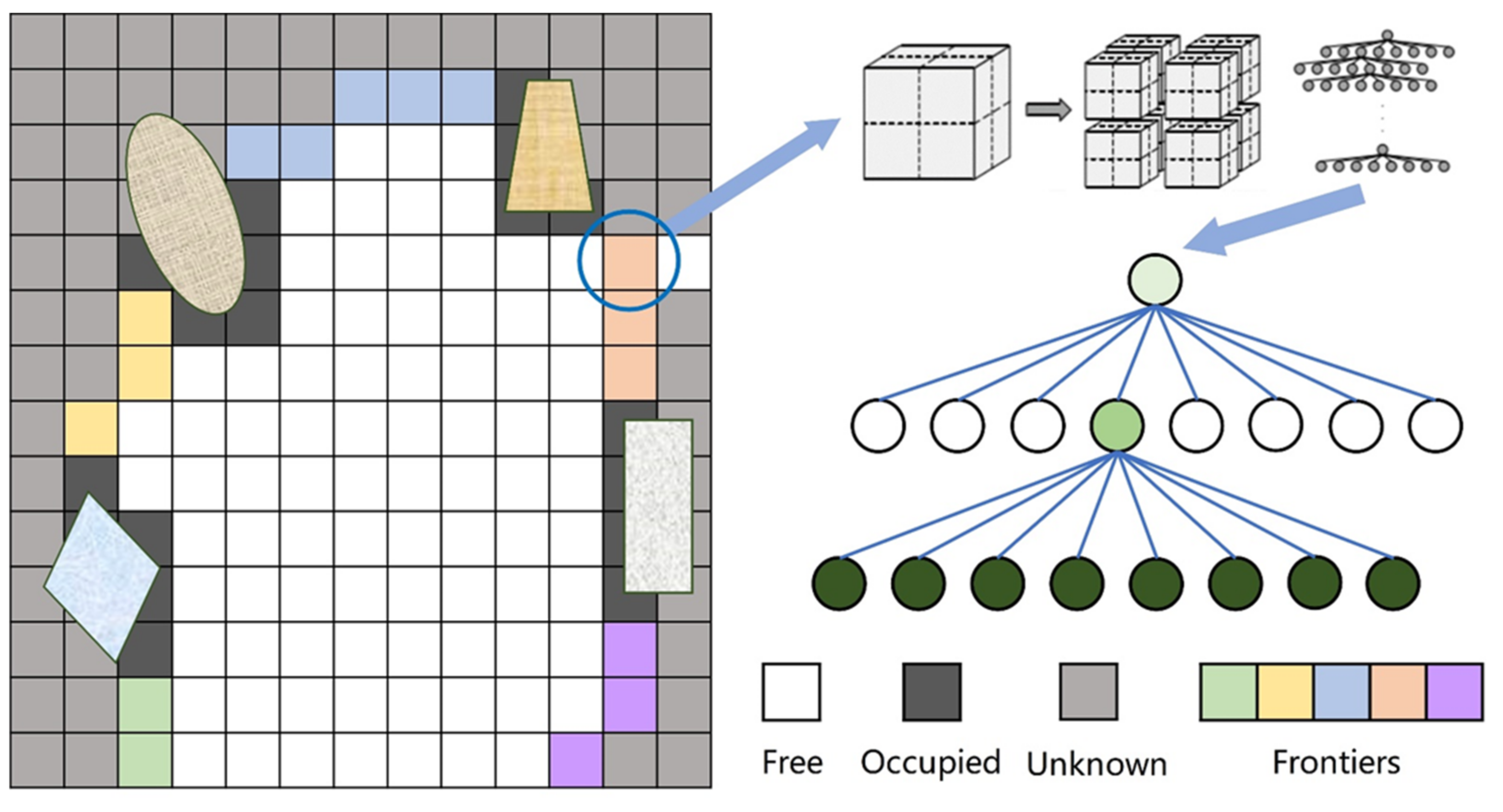
- It combines frontier-based exploration with sampling-based exploration. Via implicit voxel grouping in the octree graph representation, frontier voxels can be regarded as clusters, thereby avoiding the computationally expensive steps of frontier voxel clustering in original frontier-based methods.
- Original RRT algorithm can easily fall into a local minimal area. This paper introduced the dynamic step size and adaptive weight in UAV path planning system based on the rapid exploration tree. The purpose of planning the optimal trajectory in the task environment based on dynamic step size and adaptive weights, so as to improve search efficiency, increasing success rate and improving quality of generated paths.
- To avoid irrationality of the planned path, UAV dynamic constraints are introduced in the planning process to avoid the situation where the climbing angle and the turning angle are large. Hermite difference polynomial is used for smooth out the twisted sections of the original path.
2. Related Work
2.1. Autonomous Exploration
2.2. Path Planning
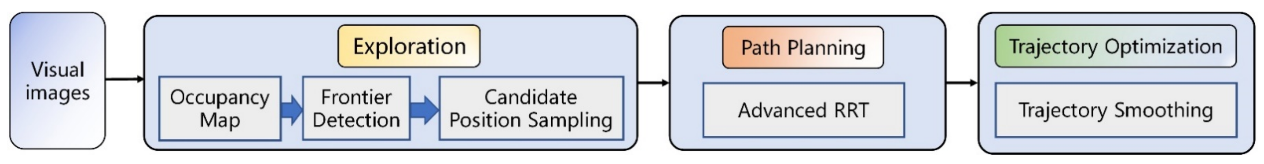
3. System Overview
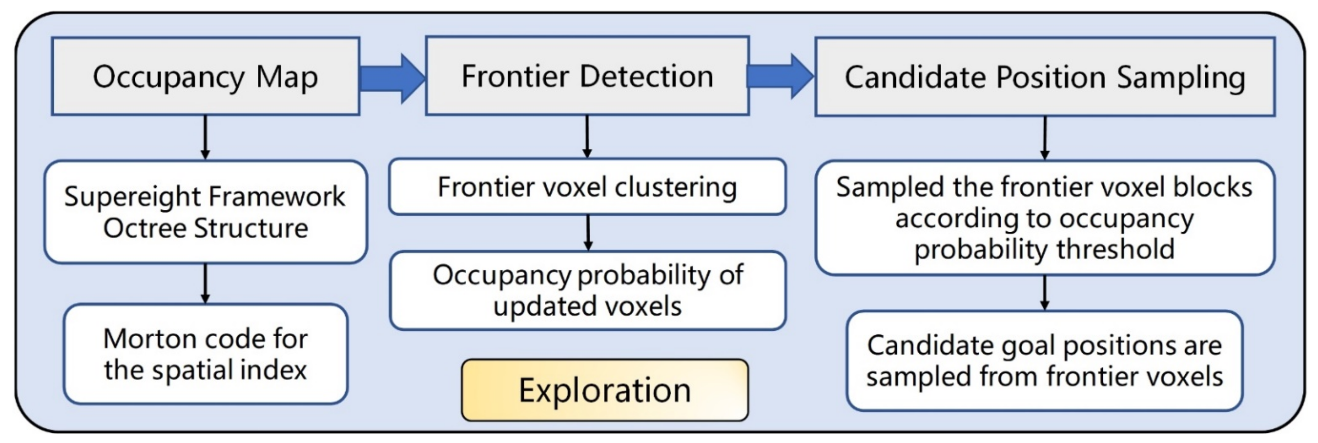
4. Exploration
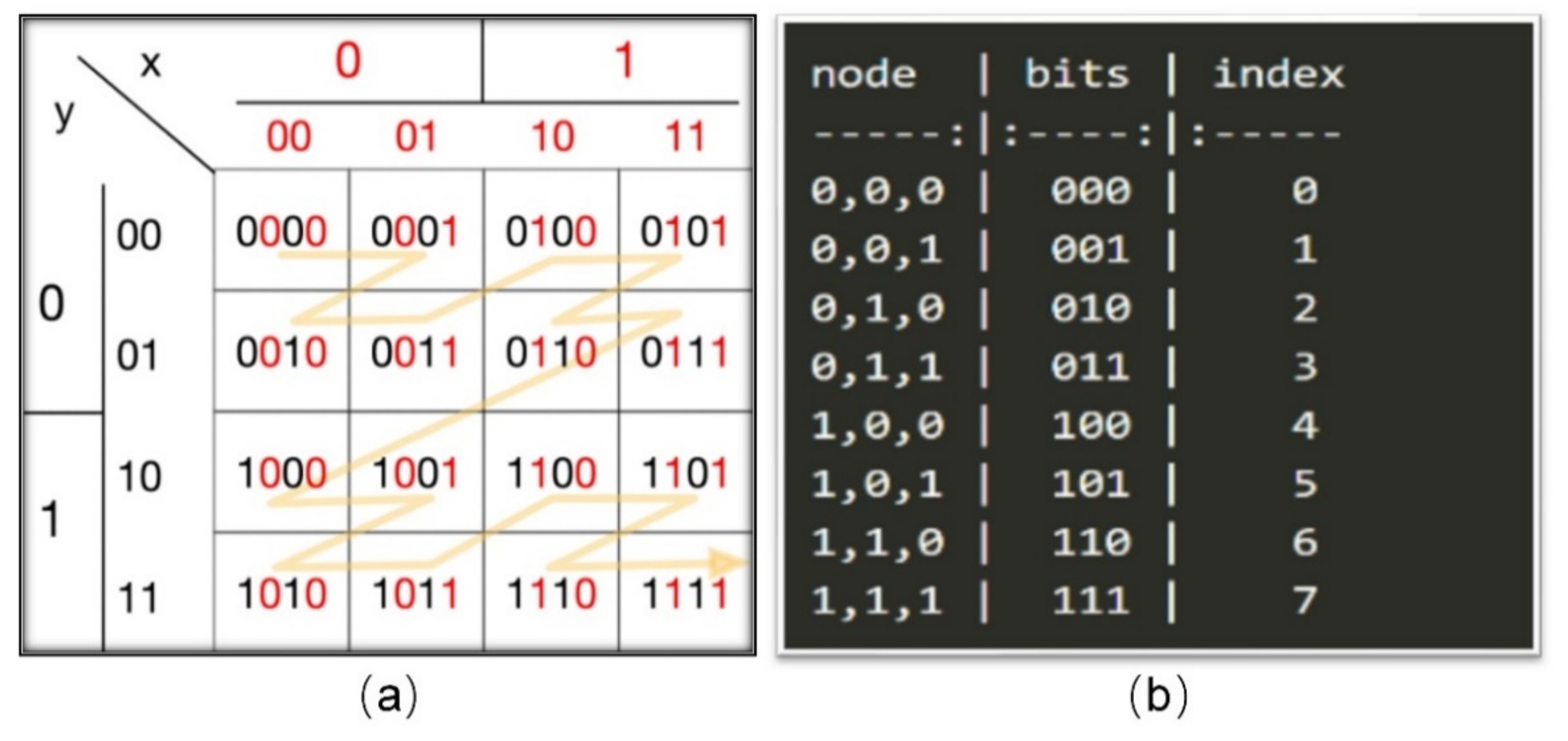
4.1. Map Representation
4.2. Frontier Detection
4.3. Candidate Position Sampling
5. Path Planning
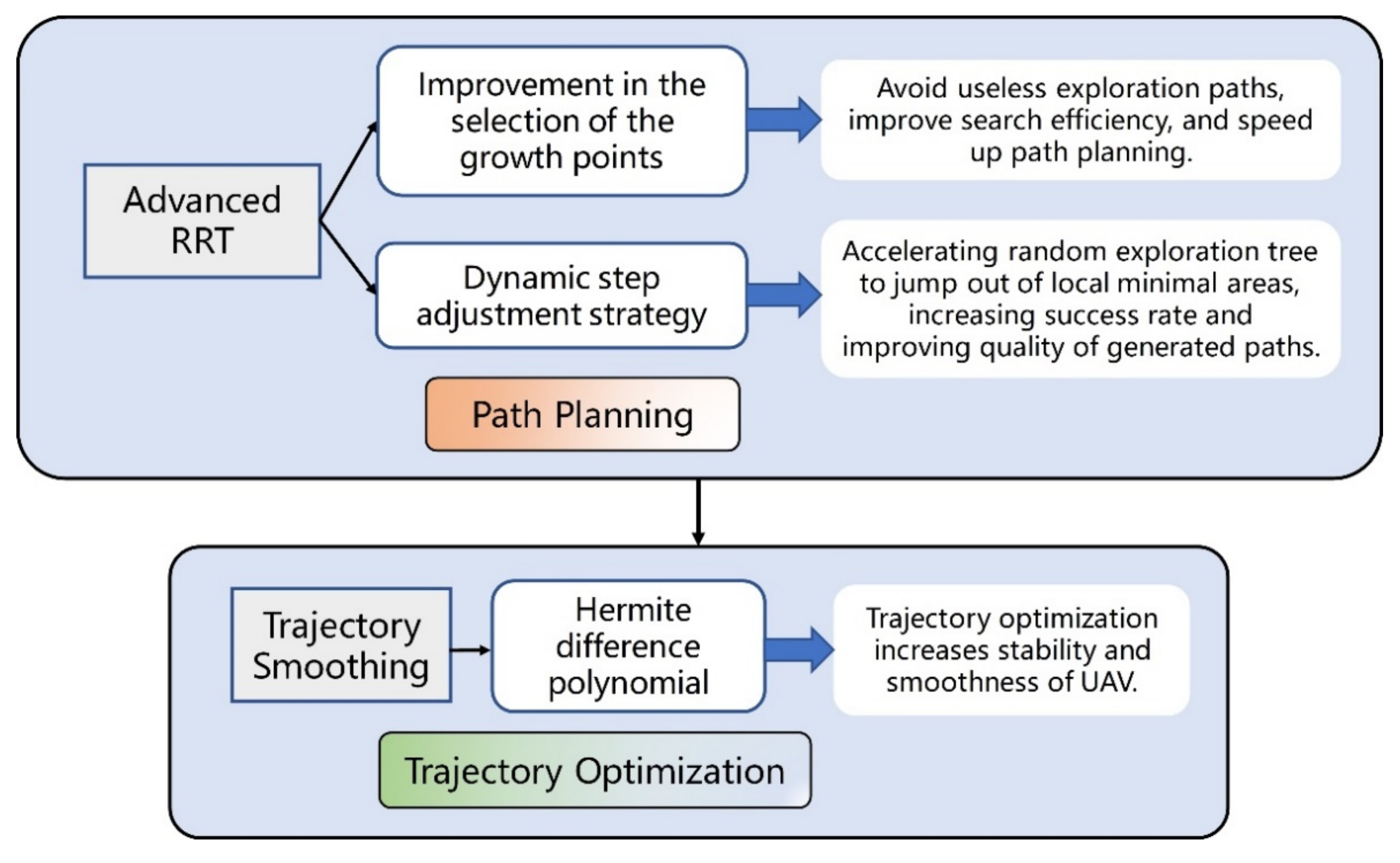
5.1. Advanced RRT
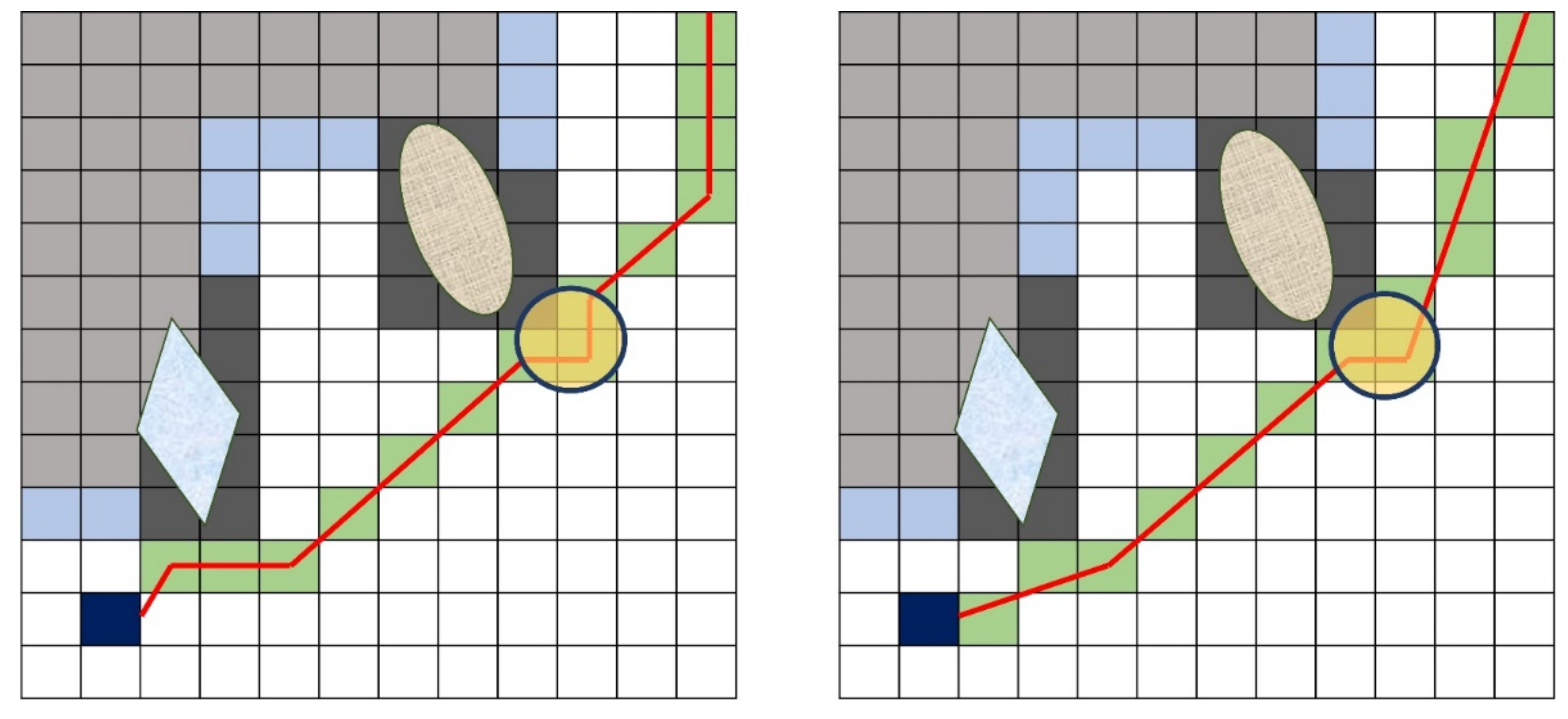
5.1.1. Improvement in the Selection of the Growth Points
5.1.2. Dynamic Step Adjustment Strategy
5.2. Improved RRT Algorithm Structure
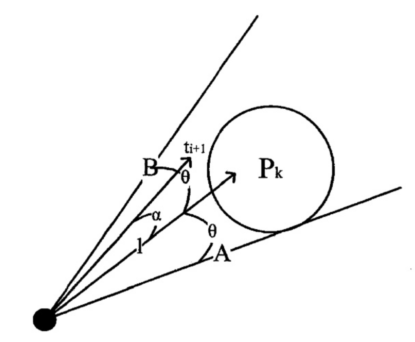
- Initialize the exploration tree T, the exploration step ds, the maximum turning angle θ, and the turning angle α.;
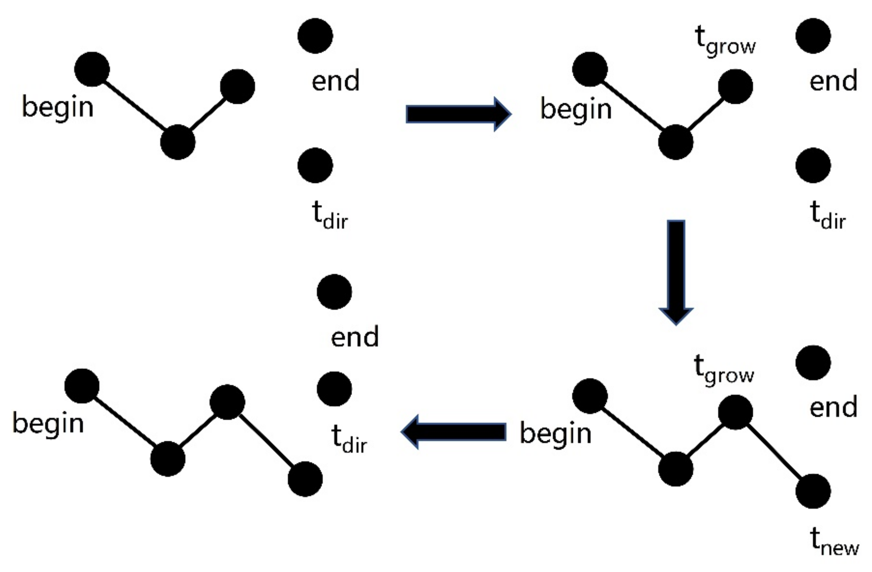
- Find the random exploration direction point tdir (tgoal and trandom are the task target point and a random point in the space, respectively, and P is a random number between 0 and 1).tdir = p∗tgoal + (1 − p) ∗ trand, (0 < p < 1)
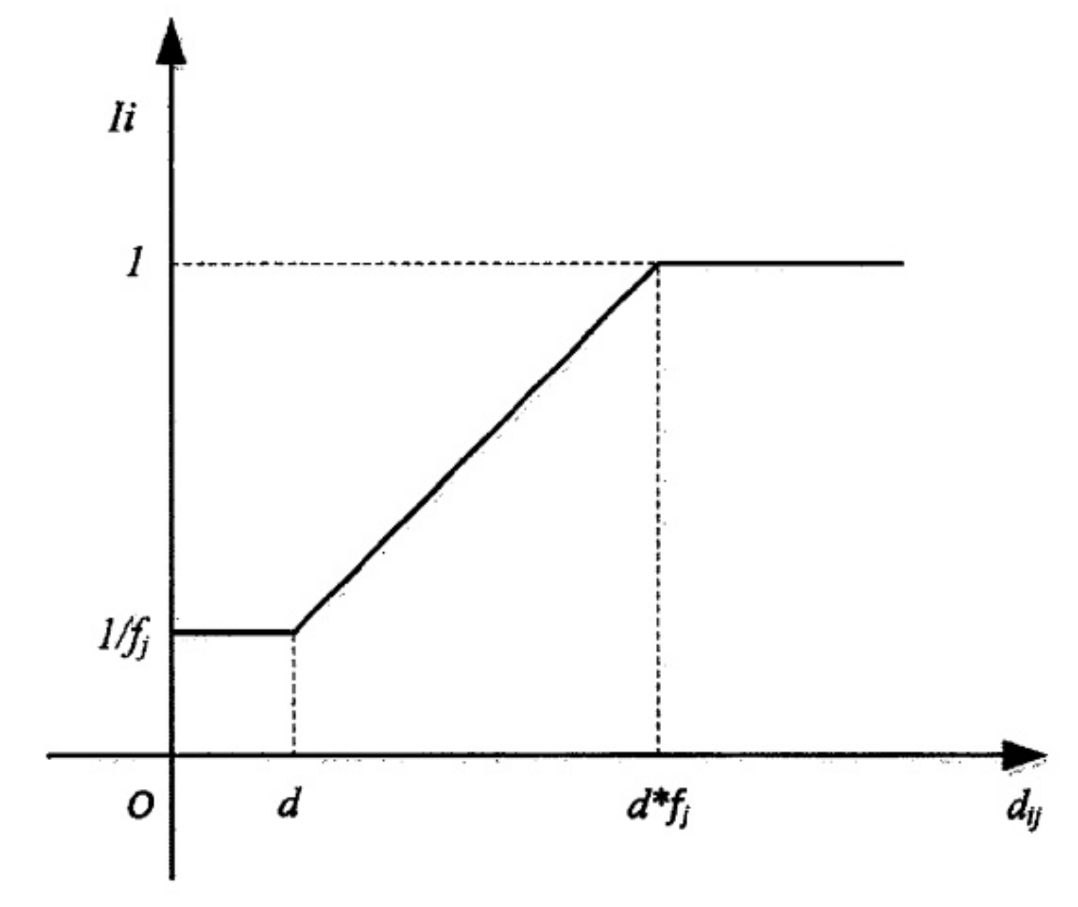
- Calculate the exploration step length d:
- Select the growth point of the tree tgrow.ωi = Ii/ditgrow = argmax(ωi), ti ∈ T
- Find the new node of the tree tnew
- Determine whether tnew is a node that has not been explored. If yes, calculate the turning angle , tj = tgrow, fj + 1, and skip to (2); otherwise, tnew is added to the exploration tree, tj = NULL, and fj = 1.
- Determine whether the target point is reached. If ‖tgoal − tnew‖ < s, the goal is reached. Otherwise, return to Equation (2). Here, s is the shortest flight distance of the UAV.
- Backtrack from the target point to the root node of the exploration tree and return to the planned path.
| Algorithm 1 Advanced RRT |
|
5.3. Trajectory Optimization
6. Experimental Results
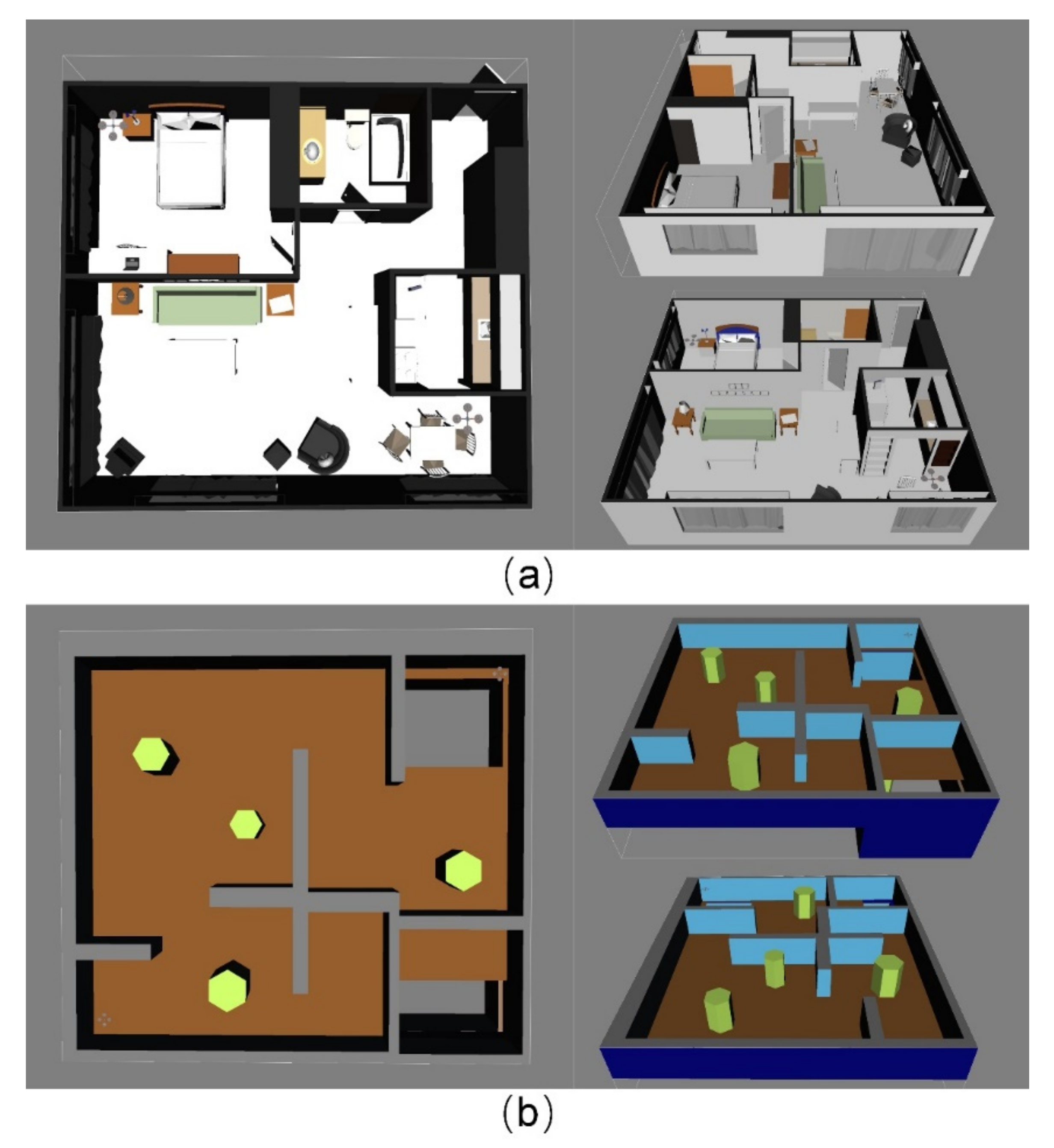
6.1. Simulation Setup
6.2. Apartment and Maze Environment Exploration Simulation Results
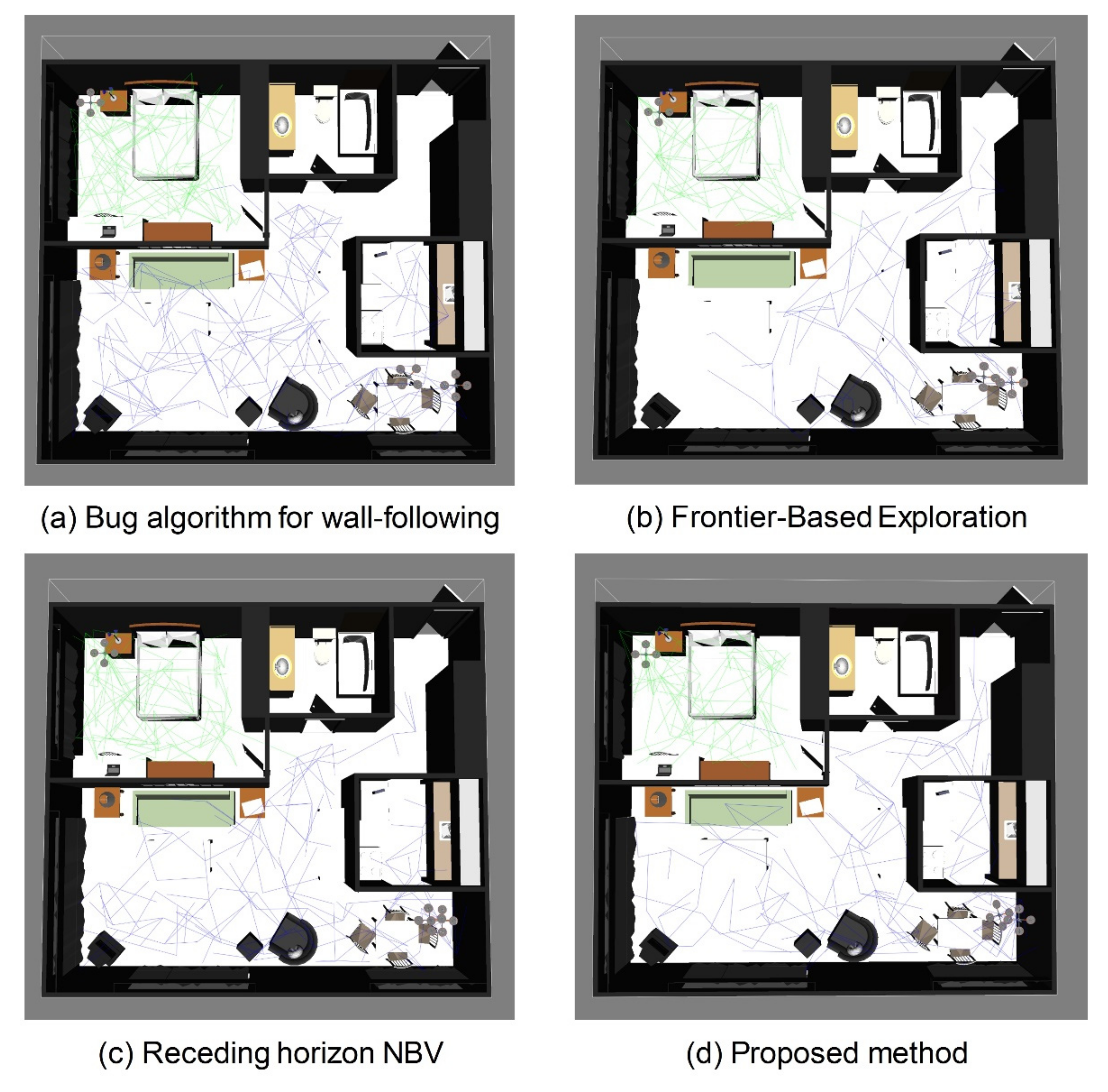
6.2.1. Apartment Environment Simulation
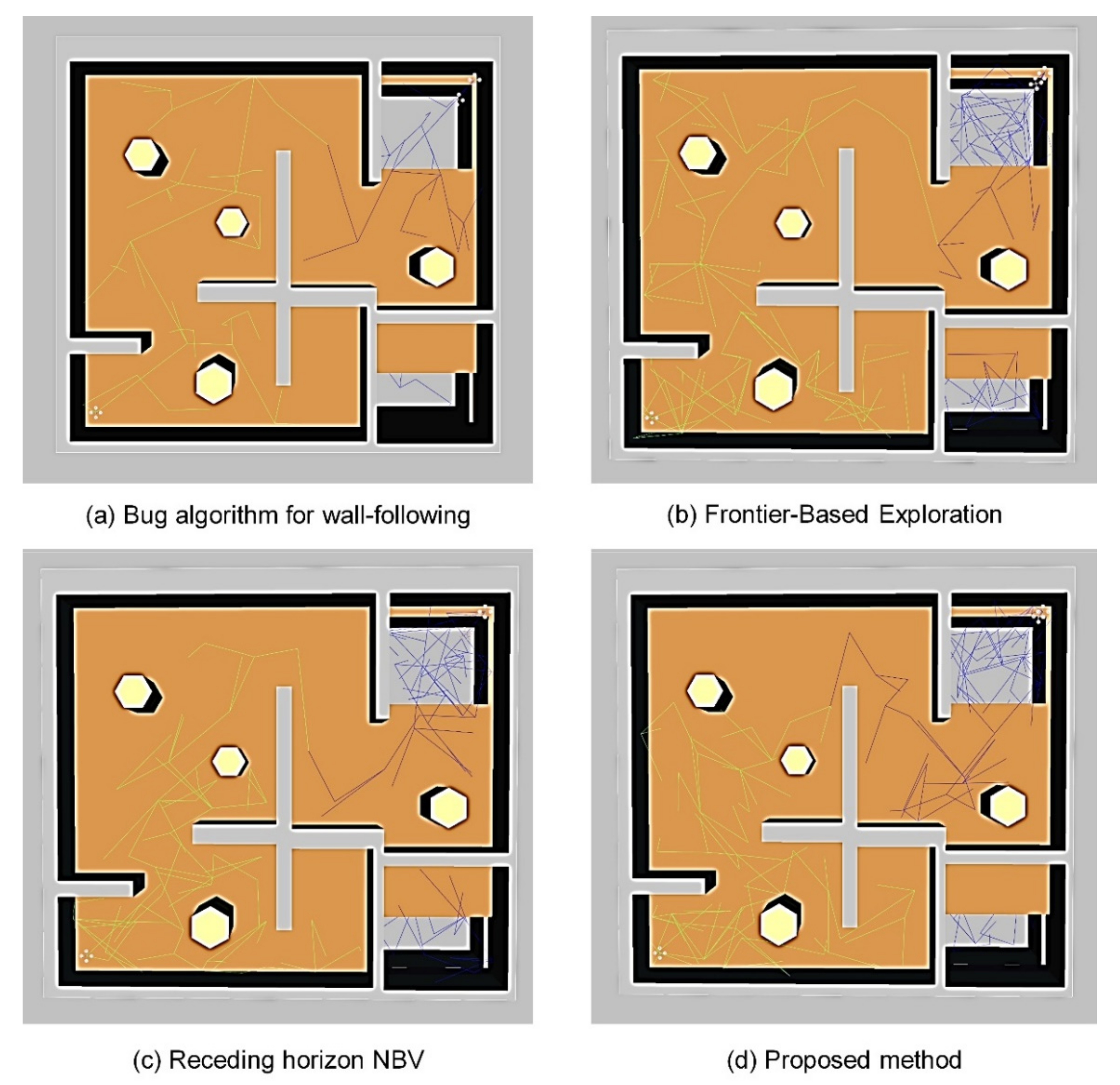
6.2.2. Maze Environment Simulation
6.3. Apartment and Maze Environment Path Planning Simulation Results
7. Conclusions and Future Work
Author Contributions
Funding
Institutional Review Board Statement
Informed Consent Statement
Data Availability Statement
Conflicts of Interest
References
- Shen, S.; Mulgaonkar, Y.; Michael, N.; Kumar, V. Multi-sensor fusion for robust autonomous flight in indoor and outdoor environments with a rotorcraft MAV. In Proceedings of the 2014 IEEE International Conference on Robotics and Automation, Hong Kong, China, 31 May–7 June 2014; pp. 4974–4981. [Google Scholar]
- Loianno, G.; Brunner, C.; McGrath, G.; Kumar, V. Estimation, control, and planning for aggressive flight with a small quadrotor with a single camera and IMU. IEEE Robot. Autom. Lett. 2016, 2, 404–411. [Google Scholar] [CrossRef]
- Liu, S.; Watterson, M.; Mohta, K.; Sun, K.; Bhattacharya, S.; Taylor, C.J.; Kumar, V. Planning dynamically feasible trajectories for quadrotors using safe flight corridors in 3-d complex environments. IEEE Robot. Autom. Lett. 2017, 2, 1688–1695. [Google Scholar] [CrossRef]
- Papachristos, C.; Kamel, M.; Popović, M.; Khattak, S.; Bircher, A.; Oleynikova, H.; Siegwart, R. Autonomous exploration and inspection path planning for aerial robots using the robot operating system. In Robot Operating System; Springer: Cham, Switzerland, 2019; pp. 67–111. [Google Scholar]
- Tang, S.; Kumar, V. A complete algorithm for generating safe trajectories for multi-robot teams. In Robotics Research; Springer: Cham, Switzerland, 2018; pp. 599–616. [Google Scholar]
- Shen, S.; Michael, N.; Kumar, V. Obtaining liftoff indoors: Autonomous navigation in confined indoor environments. IEEE Robot. Autom. Mag. 2013, 20, 40–48. [Google Scholar] [CrossRef]
- Stumberg, L.; Usenko, V.; Engel, J.; Stückler, J.; Cremers, D. From monocular SLAM to autonomous drone exploration. In Proceedings of the 2017 European Conference on Mobile Robots, Paris, France, 6–8 September 2017; pp. 1–8. [Google Scholar]
- Shen, S.; Michael, N.; Kumar, V. Autonomous indoor 3D exploration with a micro-aerial vehicle. In Proceedings of the 2012 IEEE International Conference on Robotics and Automation, Saint Paul, MN, USA, 14–18 May 2012; pp. 9–15. [Google Scholar]
- Fraundorfer, F.; Heng, L.; Honegger, D.; Lee, G.H.; Meier, L.; Tanskanen, P.; Pollefeys, M. Vision-based autonomous mapping and exploration using a quadrotor MAV. In Proceedings of the 2012 IEEE/RSJ International Conference on Intelligent Robots and Systems, Vilamoura-Algarve, Portugal, 7–12 October 2012; pp. 4557–4564. [Google Scholar]
- Song, S.; Jo, S. Surface-based exploration for autonomous 3D modelling. In Proceedings of the IEEE International Conference on Robotics and Automation, Brisbane, QLD, Australia, 21–25 May 2018; pp. 4319–4326. [Google Scholar]
- Dharmadhikari, M.; Dang, T.; Solanka, L.; Loje, J.; Nguyen, H.; Khedekar, N.; Alexis, K. Motion primitives-based path planning for fast and agile exploration using aerial robots. In Proceedings of the 2020 IEEE International Conference on Robotics and Automation, Paris, France, 31 May–31 August 2020; pp. 179–185. [Google Scholar]
- Bachrach, A.; He, R.; Roy, N. Autonomous flight in unknown indoor environments. Int. J. Micro Air Veh. 2009, 1, 217–228. [Google Scholar] [CrossRef] [Green Version]
- Yamauchi, B. A frontier-based approach for autonomous exploration. In Proceedings of the 1997 IEEE International Symposium on Computational Intelligence in Robotics and Automationm, Monterey, CA, USA, 10–11 July 1997; pp. 146–151. [Google Scholar]
- Heng, L.; Honegger, D.; Lee, G.H.; Meier, L.; Tanskanen, P.; Fraundorfer, F.; Pollefeys, M. Autonomous Visual Mapping and Exploration with a Micro Aerial Vehicle. J. Field Robot. 2014, 31, 654–675. [Google Scholar] [CrossRef]
- Connolly, C. The determination of next best views. In Proceedings of the IEEE International Conference on Robotics and Automation, St. Louis, MO, USA, 25–28 March 1985; pp. 432–435. [Google Scholar]
- Papachristos, C.; Khattak, S.; Alexis, K. Uncertainty-aware receding horizon exploration and mapping using aerial robots. In Proceedings of the 2017 IEEE International Conference on Robotics and Automation, Singapore, 29 May–3 June 2017; pp. 4568–4575. [Google Scholar]
- González-Banos, H.H.; Latombe, J.C. Navigation strategies for exploring indoor environments. Int. J. Robot. Res. 2002, 21, 829–848. [Google Scholar] [CrossRef]
- Witting, C.; Fehr, M.; Bähnemann, R.; Oleynikova, H.; Siegwart, R. History-aware autonomous exploration in confined environments using mavs. In Proceedings of the 2018 IEEE/RSJ International Conference on Intelligent Robots and Systems, Madrid, Spain, 1–5 October 2018; pp. 1–9. [Google Scholar]
- Bircher, A.; Kamel, M.; Alexis, K.; Oleynikova, H.; Siegwart, R. Receding horizon ”next-best-view” planner for 3d exploration. In Proceedings of the 2016 IEEE International Conference on Robotics and Automation, Stockholm, Sweden, 16–21 May 2016; pp. 1462–1468. [Google Scholar]
- Dashkevich, A.; Rosokha, S.; Vorontsova, D. Simulation Tool for the Drone Trajectory Planning Based on Genetic Algorithm Approach. In Proceedings of the 2020 IEEE KhPI Week on Advanced Technology, Kharkiv, Ukraine, 5–10 October 2020; pp. 387–390. [Google Scholar]
- Ge, J.; Liu, L.; Dong, X.; Tian, W. Trajectory Planning of Fixed-wing UAV Using Kinodynamic RRT* Algorithm. In Proceedings of the 2020 10th International Conference on Information Science and Technology (ICIST), London, UK, 9–15 September 2020; pp. 44–49. [Google Scholar]
- Kim, S.; Sreenath, K.; Bhattacharya, S.; Kumar, V. Optimal trajectory generation under homology class constraints. In Proceedings of the 2012 IEEE 51st IEEE Conference on Decision and Control, Maui, HI, USA, 10–13 December 2012; pp. 3157–3164. [Google Scholar]
- Hart, P.E.; Nilsson, N.J.; Raphael, B. A Formal Basis for the Heuristic Determination of Minimum Cost Paths. IEEE Trans. Syst. Sci. Cybern. 1968, 4, 100–107. [Google Scholar] [CrossRef]
- Ferguson, D.; Stentz, A. Using interpolation to improve path planning: The Field D* algorithm. J. Field Robot. 2006, 23, 79–101. [Google Scholar] [CrossRef] [Green Version]
- Ferguson, D.; Anthony, S. Field D*: An interpolation-based path planner and replanner. In Robotics Research; Springer: Berlin/Heidelberg, Germany, 2007; pp. 239–253. [Google Scholar]
- Kavraki, L.E.; Svestka, P.; Latombe, J.C.; Overmars, M.H. Probabilistic roadmaps for path planning in high-dimensional configuration spaces. IEEE Trans. Robot. Autom. 1996, 12, 566–580. [Google Scholar] [CrossRef] [Green Version]
- LaValle, S.M.; Kuffner, J., Jr. Randomized kinodynamic planning. Int. J. Robot. Res. 2001, 20, 378–400. [Google Scholar] [CrossRef]
- Geraerts, R.; Mark, H.O. A comparative study of probabilistic roadmap planners. In Algorithmic Foundations of Robotics V; Springer: Berlin/Heidelberg, Germany, 2004; pp. 43–57. [Google Scholar]
- Karaman, S.; Frazzoli, E. Incremental sampling-based algorithms for optimal motion planning. In Robotics Science and Systems; Zaragoza, Spain, June 2010; Volume 104. [Google Scholar]
- Adiyatov, O.; Varol, H.A. Rapidly-exploring random tree based memory efficient motion planning. In Mechatronics and Automation (ICMA); Nazarbayev University: Takamatsu, Japan, August 2013; pp. 354–359. [Google Scholar]
- Gammell, J.D.; Srinivasa, S.S.; Barfoot, T.D. Informed RRT*: Optimal Sampling-based Path Planning Focused via Direct Sampling of an Admissible Ellipsoidal Heuristic. In Proceedings of the 2014 IEEE/RSJ International Conference on Intelligent Robots and Systems, Chicago, IL, USA, 14–18 September 2014; pp. 2997–3004. [Google Scholar]
- Kuffner, J.J.; LaValle, S.M. RRT-connect: An efficient approach to single-query path planning. In Proceedings of the IEEE International Conference on Robotics and Automation, San Francisco, CA, USA, 24–28 April 2000; pp. 995–1001. [Google Scholar]
- Kuwata, Y.; Teo, J.; Fiore, G.; Karaman, S.; Frazzoli, E.; How, J.P. Real-time motion planning with applications to autonomous urban driving. IEEE Trans. Control Syst. Technol. 2009, 17, 1105–1118. [Google Scholar] [CrossRef]
- Vespa, E.; Nikolov, N.; Grimm, M.; Nardi, L.; Kelly, P.H.; Leutenegger, S. Efficient octree-based volumetric SLAM supporting signed-distance and occupancy mapping. IEEE Robot. Autom. Lett. 2018, 3, 1144–1151. [Google Scholar] [CrossRef] [Green Version]
- Spitzbart, A. A generalization of Hermite’s interpolation formula. Am. Math. Mon. 1960, 67, 42–46. [Google Scholar] [CrossRef]


| Autonomous Exploration Algorithm | Advantage | Difficulties |
|---|---|---|
| Frontier-based exploration [13] | Perform well in 2-dimension environment | Redundant frontiers generating due to environmental occlusion and noise |
| VFH + plus bug algorithm [14] | Perform well in sparse environments | Require the planner knows the location of the goal and assume the robot has perfect positioning |
| NBV [15] | High exploration coverage | Random sampling not always detect unexplored areas fast |
| Bircher’s NBV [16] | Minimize the uncertainty of robot positioning and tracking marks | High computational complexity and long exploration time. |
| Directly sample candidate NBV [17] | Proposed the term of safe region, higher in exploration coverage | High precision of relative positioning is required |
| Path Planning Algorithm | Advantage | Difficulties |
|---|---|---|
| A Star [23] | Informed search algorithm high; efficiency in heuristic planning; | Optimal search path cannot be guaranteed in multiple minimum values |
| D Star [24] | Incremental search algorithm; rapid planning in re-planning | Consumes a lot of search and calculation time |
| PRM [26] | Track planning using random road map method; easy to find the optimal trajectory | Cannot be applied to real-time planning |
| RRT [27] | Effectively solve high-dimensional space and complex constraints | Random search is not sensitive to complex environment |
| Informed RRT Star [31] | Less dependence on the dimension and domain | Cannot focus the search when associated prolate hyperspheroid is large |
| RRT-Connect [32] | High Search speed and search efficiency | Expensive in high dimension; difficult to find a path in a narrow environment |
| Closed-loop RRT [33] | Well performance in dynamic unstable environment | Not convenient to address the situation of a complex terrain |
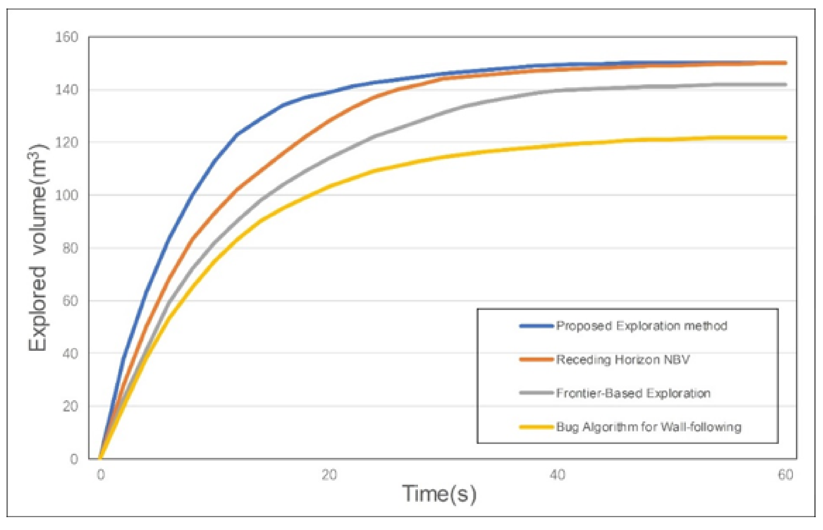
| Algothrim | Frontier-Based Exploration [13] | Receding Horizon NBV [18] | Bug Algorithm for Wall-Following [14] | Proposed Method |
|---|---|---|---|---|
| Flight time (s) | 15.29 | 16.78 | 21.52 | 14.37 |
| Coverage (&) | 93.73 | 98.96 | 89.44 | 99.27 |
| Algothrim | Frontier-Based Exploration [13] | Receding Horizon NBV [18] | Bug Algorithm for Wall-Following [14] | Proposed Method |
|---|---|---|---|---|
| Flight time (s) | 43.59 | 52.31 | 47.37 | 37.69 |
| Coverage (&) | 87.17 | 94.75 | 74.46 | 93.27 |
Publisher’s Note: MDPI stays neutral with regard to jurisdictional claims in published maps and institutional affiliations. |
© 2021 by the authors. Licensee MDPI, Basel, Switzerland. This article is an open access article distributed under the terms and conditions of the Creative Commons Attribution (CC BY) license (https://creativecommons.org/licenses/by/4.0/).
Share and Cite
Zhao, L.; Yan, L.; Hu, X.; Yuan, J.; Liu, Z. Efficient and High Path Quality Autonomous Exploration and Trajectory Planning of UAV in an Unknown Environment. ISPRS Int. J. Geo-Inf. 2021, 10, 631. https://0-doi-org.brum.beds.ac.uk/10.3390/ijgi10100631
Zhao L, Yan L, Hu X, Yuan J, Liu Z. Efficient and High Path Quality Autonomous Exploration and Trajectory Planning of UAV in an Unknown Environment. ISPRS International Journal of Geo-Information. 2021; 10(10):631. https://0-doi-org.brum.beds.ac.uk/10.3390/ijgi10100631
Chicago/Turabian StyleZhao, Leyang, Li Yan, Xiao Hu, Jinbiao Yuan, and Zhenbao Liu. 2021. "Efficient and High Path Quality Autonomous Exploration and Trajectory Planning of UAV in an Unknown Environment" ISPRS International Journal of Geo-Information 10, no. 10: 631. https://0-doi-org.brum.beds.ac.uk/10.3390/ijgi10100631