Article

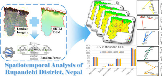
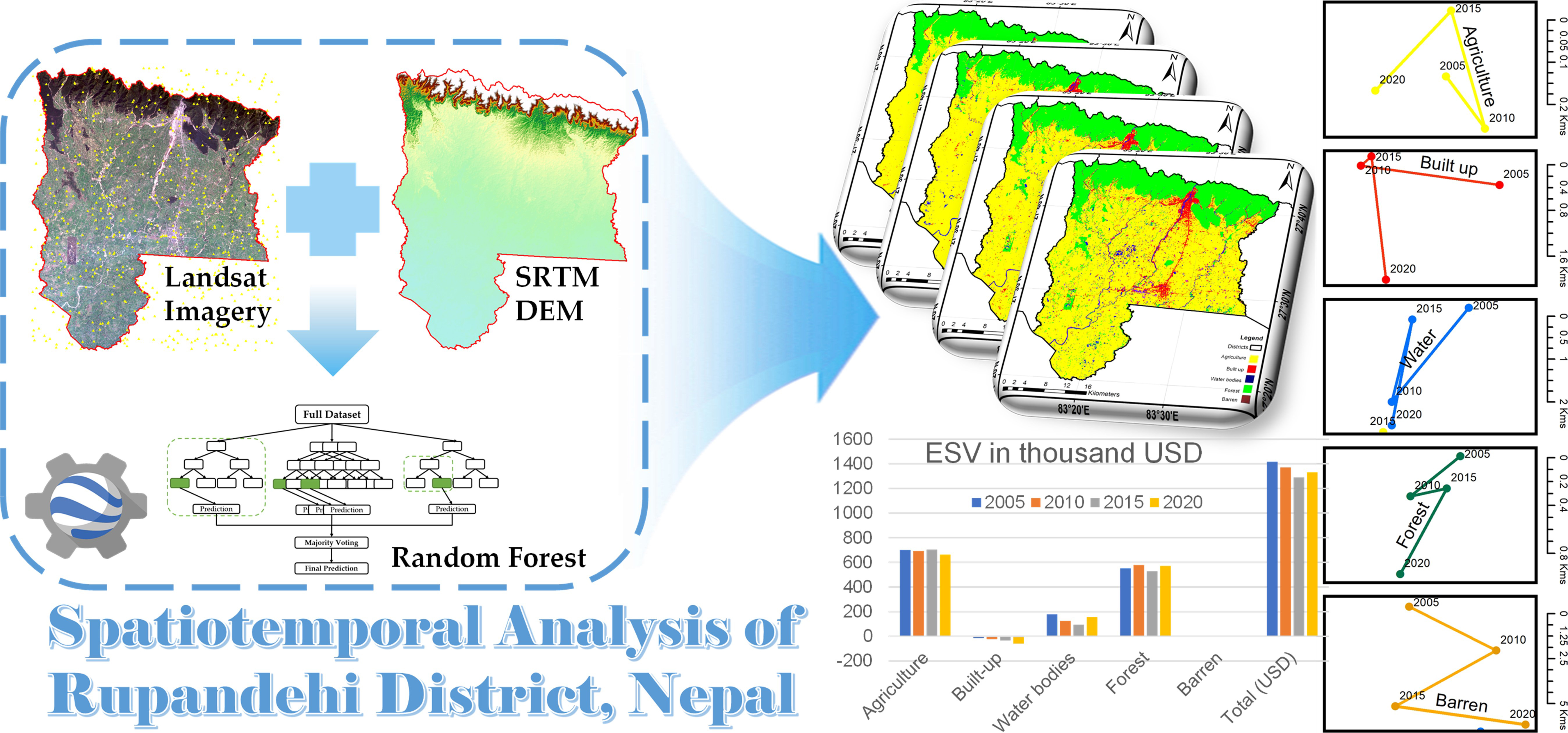
Spatiotemporal Analysis of Land Cover and the Effects on Ecosystem Service Values in Rupandehi, Nepal from 2005 to 2020

1
Department of Civil and Geomatics Engineering, Pashchimanchal Campus, Tribhuvan University, Pokhara 33700, Nepal
2
Kanchan Rural Municipality, Government of Nepal, Gajedi, Rupandehi 32900, Nepal
3
Survey Department, Government of Nepal, Minbhawan, Kathmandu 44600, Nepal
4
Institute of Transportation Studies, University of California Davis, Davis, CA 95616, USA
*
Author to whom correspondence should be addressed.
ISPRS Int. J. Geo-Inf. 2021, 10(10), 635; https://0-doi-org.brum.beds.ac.uk/10.3390/ijgi10100635
Submission received: 2 August 2021 / Revised: 13 September 2021 / Accepted: 16 September 2021 / Published: 23 September 2021

Abstract

:
Land cover (LC) is a crucial parameter for studying environmental phenomena. Cutting-edge technology such as remote sensing (RS) and cloud computing have made LC change mapping efficient. In this study, the LC of Rupandehi District of Nepal were mapped using Landsat imagery and Random Forest (RF) classifier from 2005 to 2020 using Google Earth Engine (GEE) platform. GEE eases the way in extracting, analyzing, and performing different operations for the earth’s observed data. Land cover classification, Centre of gravity (CoG), and their trajectories for all LC classes: agriculture, built-up, water, forest, and barren area were extracted with five-year intervals, along with their Ecosystem service values (ESV) to understand the load on the ecosystem. We also discussed the aspects and problems of the spatiotemporal analysis of developing regions. It was observed that the built-up areas had been increasing over the years and more centered in between the two major cities. Other agriculture, water, and forest classes had been subjected to fluctuations with barren land in the decreasing trend. This alteration in the area of the LC classes also resulted in varying ESVs for individual land cover and total values for the years. The accuracy for the RF classifier was under substantial agreement for such fragmented LCs. Using LC, CoG, and ESV, the paper discusses the need for spatiotemporal analysis studies in Nepal to overcome the current limitations and later expansion to other regions. Studies such as these help in implementing proper plans and strategies by district administration offices and local governmental bodies to stop the exploitation of resources.

Graphical Abstract

1. Introduction

Land cover (LC) is an important parameter to study and track the local, regional, and global changes of the earth’s surface. It has been a crucial variable for different studies such as climate change, food security, environmental studies, conservational strategies, hydrology, and landscape planning [1,2,3,4]. LC, being subjected to natural phenomena and anthropogenic causes of land use, is very dynamic [2,3]. The changes in the constitution of LC represent one of the most significant sources of system changes at local, provincial, and worldwide scales [5]. To accomplish the United Nations’ Sustainable Development Goals (SDGs), timely and higher resolution LC data are critical [6].
The long-term earth observation data record is a tool for analyzing the land use and land cover changes (LCC) [7]. Remote Sensing has been a useful aid in studying the patterns of LC with a decreased cost and less effort [2]. The easily accessible and freely available satellite imageries have assisted in studying the LC patterns at a regional and global scale, which would have been difficult, if not impossible. Various global LC data have been produced over the years, such as GLC2000 [8], MCD12, and GLCNMO, GlobCover [9], IGBP DISCover [10], MODIS Collection 5 global land cover [11], Global Land Surface Satellite Global Land Cover (GLASS-GLC) [12], GLC30 [13], GLC10 [6], ESA CCI Land Cover time-series [8], ESRI 10 m [14], etc. While some researchers are concentrated on a local or regional level to map out specific phenomena, for example, meteorology [15], future prediction [16,17], urban heat islands [18], climate change [19], water [20], forest [21] and biodiversity [22], and agricultural monitoring [23], current studies are also focused on improvements such as finer resolution and classification procedures [1,24,25,26].
Image Classification is the basis of LC, in which we assign LC classes to a multiband raster image. Image Classification in remote sensing is broadly categorized into the following three types: pixel-wise classification, sub-pixel-wise classification, and object-based image classification. Pixel-wise classification treats each pixel as pure and is labeled as a single land use-LC type based on the spectral signature and their derivatives such as vegetation indices [27], which are further divided into an unsupervised and supervised classification. Unsupervised classification, which is based on the principle of creating clusters and assigning classes, has been used in various studies [24,25,28,29,30]. Conversely, supervised classification is based on taking samples as training data and applying them to classify [31]. While the sub-pixel classification works to address the mixed pixel problem for coarse resolution satellite images, by treating the pixel as mixed and considering the areal proportion of each class [26,32], object-based image analysis is centered on generating image objects through image segmentation and performing the image classification on objects with different geometries rather than pixels [33,34,35].
It has been evident from the review that different types of satellite images and classification algorithms have been used and the choice is undoubtedly influenced by research objective and questions to be addressed by the work. Stephens and Diesing [36] tested the following six supervised classifiers: Classification Trees, Support Vector Machines, k-Nearest Neighbor, Neural Networks, Random Forest (RF), and Naive Bayes, and found good accuracy for tree-based methods and Naive Bayes. RF is a set of tree predictors; therefore, each tree depends on the value of an independently sampled random vector, and all the trees in the forest have the same distribution [37]. RF also performed well for the LC classification of a multi-source remote sensing and geographic data set in a study conducted by Gislason et al. [38]. Eisavi et al. [39] considered different scenarios for the LC mapping using RF, with the inclusion of land surface temperature data along with spectral data, and found the approach worked best for selected features over using just spectral signatures. Therefore, RF was used as a classification method for our work as well, in which we used spectral signatures along with derived indices and topography data: slope and elevation as input parameters.
Google Earth Engine (GEE), which is a cloud computing platform, has eased in extracting, analyzing, and performing different operations for the earth’s observed data. It has been employed in different regions of the world to monitor the vegetation, water resources, and tracking the changes in land cover. As GEE is technologically robust and is an open resource containing historical images, it has become increasingly popular in LULC mapping. In the Asian region as well, it has been adopted in the countries such as India [40], Bangladesh [41], Singapore [42], China [43,44,45], Cambodia [46], Nepal [47], etc. GEE has also been applied in understanding the changes in land cover at the regional level such as in Central Asia [48] and the Tigris-Euphrates basin of the Middle East [49]. Automation in land cover mapping has also been possible due to the cloud computing feature of GEE. Xie et al. [50] proposed an automatic land cover classification method using time-series Landsat data using an International Geosphere-Biosphere Program (IGBP) classification scheme (Automatic Land-Cover Mapping).
In addition to understanding the present status of LC, it is equally important to track the motion of the center of change of the specific LC over the years. In the last years, with the growing urbanization, there have been significant changes in the types of regional land use. Therefore, the analysis of the central displacement of LC can help understand the development of the region and provide references for resource management and territorial planning [51]. For this purpose, a shift of the center of gravity (CoG) of the particular LC class has been studied [51,52,53]. The CoG models also help to explain regional shifts along the development axes [53].
Ecosystem services provide the basis for human life that are directly and indirectly contributing to human well-being and sustenance. The services range from filtering air and water by plants to decomposing wastes by microbes. These ecosystem services have been broadly grouped into the following four categories: provisioning, regulating, supporting, and cultural. With rapid development, Chinese researchers have been also using Ecosystem Service Value (ESV), an approach to assign monetary values to an ecosystem and its key ecosystem goods and services. Since Costanza et al. [54] published their article on the global value of ecosystem services, it has increasingly become more common and has been adapted in different areas modifying the coefficients of ESV [55,56,57,58]. A total of 17 types of ecosystem services were integrated into the original article by Costanza et al. [54], including climate regulation, water regulation, nutrient cycling, genetic resources, and culture. Moreover, the land is also classified into ecological land and non-ecological land, divided based on the positive or negative impacts on the ecosystem. Ecological land is the land type providing basic ecosystem services, includes non-built-up areas such as agriculture, water bodies, forest, grassland, and thus, has a high ESV. In contrast, non-ecological land is an imperious, built-up area, thus weakening the ecosystem services [59]. With the population and urbanization pressure, the richest and diversified ecosystems are under a great threat. For instance, it was reported in 2018 that wetlands are declining three times faster than forests [60]. Thus, a study of ESV could help concerned stakeholders in understanding the rapid trend of urbanization, its severe environmental effects, and the load on the ecosystem.
Rupandehi, bordering its entire southern boundary with India, is a major corridor for the economic trade between Nepal and India. Being an economic hub, the district is facing the problem of managing urban growth. Home to happening towns, the district has undergone some remarkable changes and it has become extremely crucial to monitor the changes it has experienced or will experience in the future. While there have been some studies on the LC, they are generally at a national level [3,61]. The district is composed of a large percentage of agricultural land, followed by forest cover. Due to the result of unmanaged urbanization, the area has been severely affected by land fragmentation. This has resulted in improper drainage and flooding. Our study aims to provide LC and the pattern of a centroidal shift of the LC, which can help in curbing the effects, and present plans for tackling such situations. As the changes in the past and present conditions of the district are not known, it becomes extremely crucial to monitor the changes, as it can face severe drought and other climate crises in the future. Therefore, a detailed study on the spatiotemporal analysis of the LC is a must for a rapidly growing urban region such as Rupandehi.
The study focuses on classifying the LC of the Rupandehi District into five broad classes (agriculture, built-up, water bodies, forest, and barren) based on spectral information from Landsat Sensor using the RF algorithm. The major objectives are (1) to explore the spatiotemporal change of the Rupandehi District from 2005–2020, (2) to analyze the CoG trajectory of the land cover classes, (3) to calculate and analyze the ESV of individual LC classes and the whole district, and (4) to discuss the aspects and problems of the spatiotemporal analysis of developing regions. To the best of our knowledge, this is the first study that utilizes GEE, CoG, and ESV to understand the spatiotemporal analysis in the study area. Additionally, the workflow can be adopted in other places to quantity land changes and econometrics.

2. Materials and Method
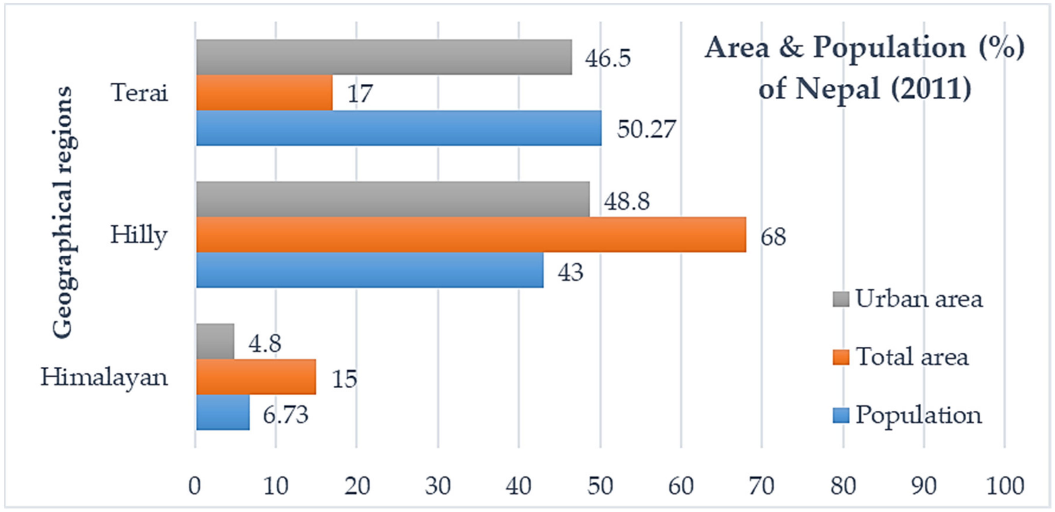
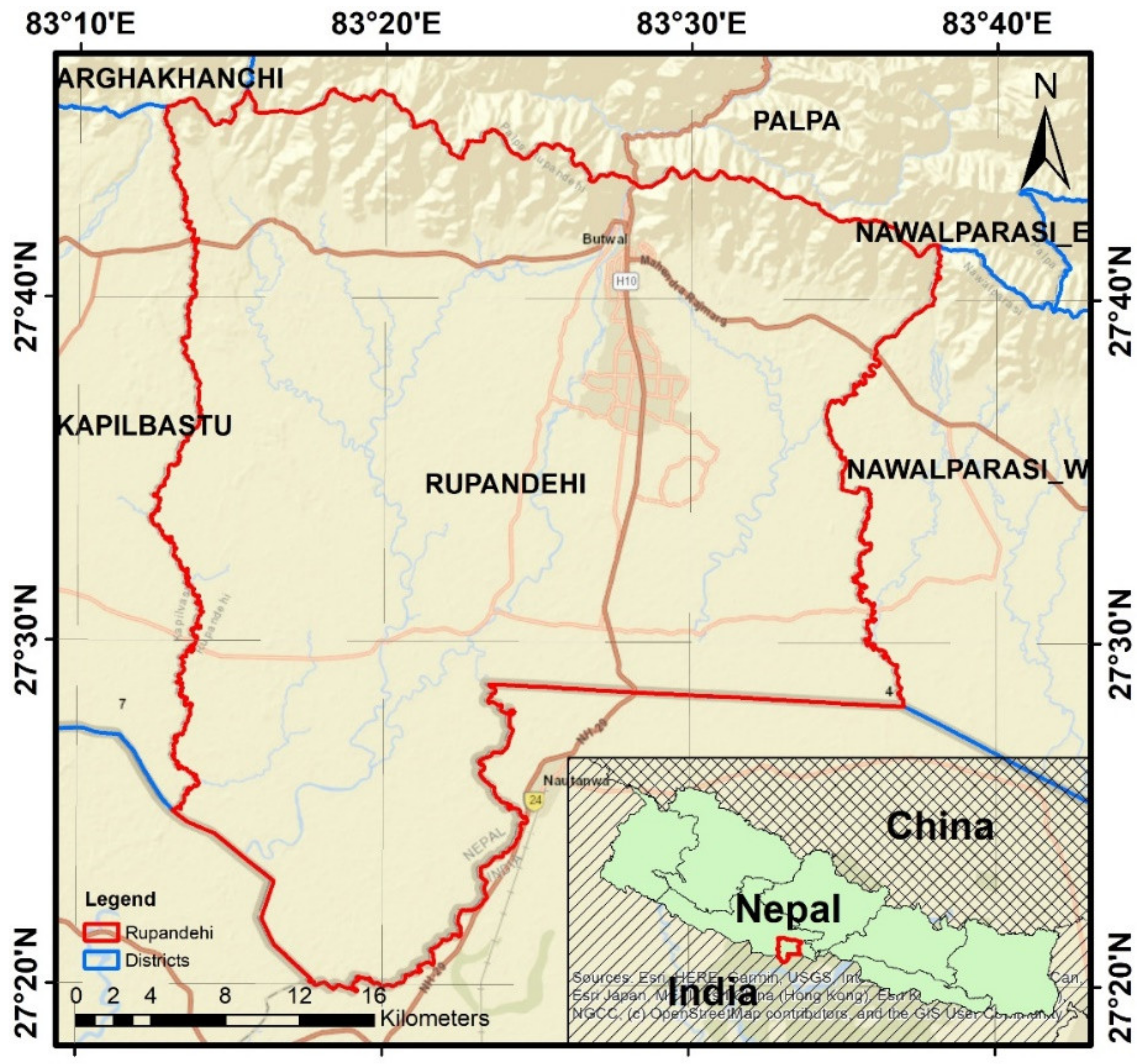
2.1. Study Area

Nepal, being one of the ten least urbanized countries in the world, is also one of the top ten fastest urbanizing countries [62]. Due to the concentration of educational and health facilities, and growing employment opportunities in Terai and major cities of valleys, there has been an upward trend of people migrating [63]. The Maoist Insurgency and the Madhesh Movement also had a significant impact on urbanization development [64]. This has led to uncontrolled population growth in the plains and valleys, resulting in unmanaged urbanization. Terai, being home to a large percentage of agricultural and forested land, is possessed by a great threat of haphazard development. Figure 1 shows the status of an urban area and population percentage in three different geographical regions (Himalayan, Hilly, and Terai). Without proper plans, the current trend would result in a sharp decline of arable land and deterioration of forests.
Figure 2 shows the study area, which is the Rupandehi District located in the Lumbini Province of Nepal. It is the third most populated district of Nepal. It covers an area of 1360 km2. Almost 60.2% of the area of the Rupandehi District is covered by agricultural land. The district lies in the southwestern part of Nepal. It shares a border with Nawalparasi District in the east, Kapilvastu District in the west, Palpa District in the north, and India in the south. The elevation of the district is between 100 and 1229 m from sea level. Of the area of Rupandehi District, 16.1% is in Churia Range and the rest is in the Terai region. It has major rivers such as Tinau and Rohini that are the source of water for its people. Most of the area of the Rupandehi District has a lower tropical climate (89.3%). It has two of the major economic hubs of Nepal: Bhairahawa and Butwal. Not only economically, but the Rupandehi District is also historically and culturally important. For the past many years, Rupandehi District has faced rapid LCC due to the migration of people from hilly to terai regions in search of flat cultivable land. It is very important to study the LCC pattern of the Rupandehi District.
The spatiotemporal analysis of LCCs for the chosen study area, i.e., Rupandehi District is still not quantified. Using Landsat Imagery in the GEE platform, LCs were derived for different years. Figure 3 shows the workflow of this study. Annual cloud-free composites were obtained for the Landsat imageries for the years 2005, 2010, 2015, and 2020. Initially, unsupervised classification (clustering) was conducted to randomly create reference points that help in capturing the variability in pixels. In addition to the surface reflectance of the bands, different indices were also derived and used as input parameters for the RF. Topographic information such as elevation and slope derived from shuttle radar topography mission (SRTM) digital elevation model (DEM) was also given as input, as they also helped in accurately classifying imageries by obviating the effect of shadows from hills and buildings. To ensure the points have been assigned the right classes, it was overlayed with very high-resolution imagery from Google Earth Pro (GEP) and cross-checked with expert knowledge. The total points obtained were randomly divided into two sets of testing and validation. The classified maps were, then, assessed based on the validation set by generating a confusion matrix. Based on obtained LC areas, shifts in the CoG and ESV and spatiotemporal changes were analyzed.

2.2. Land Cover Classification

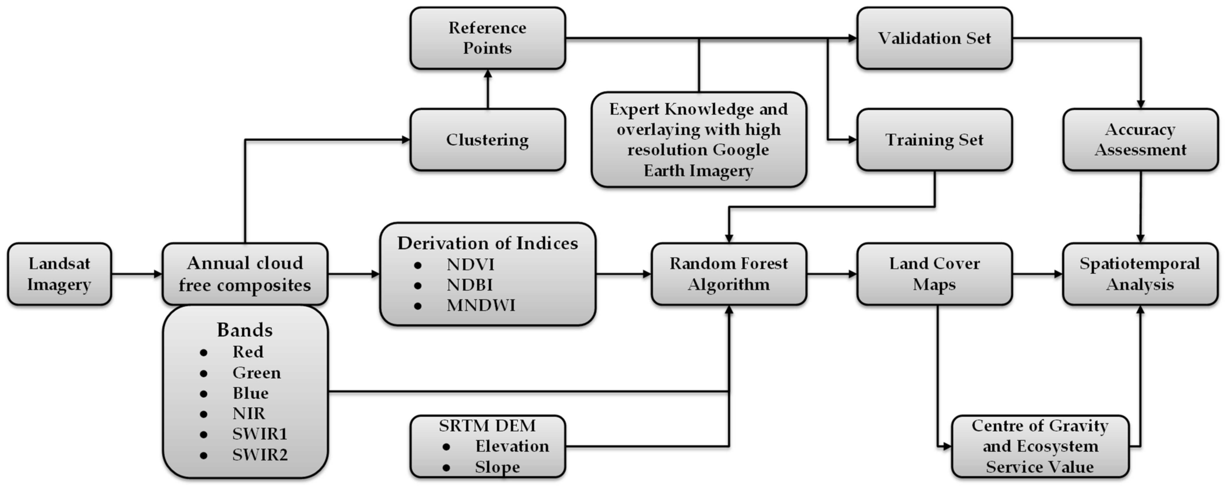
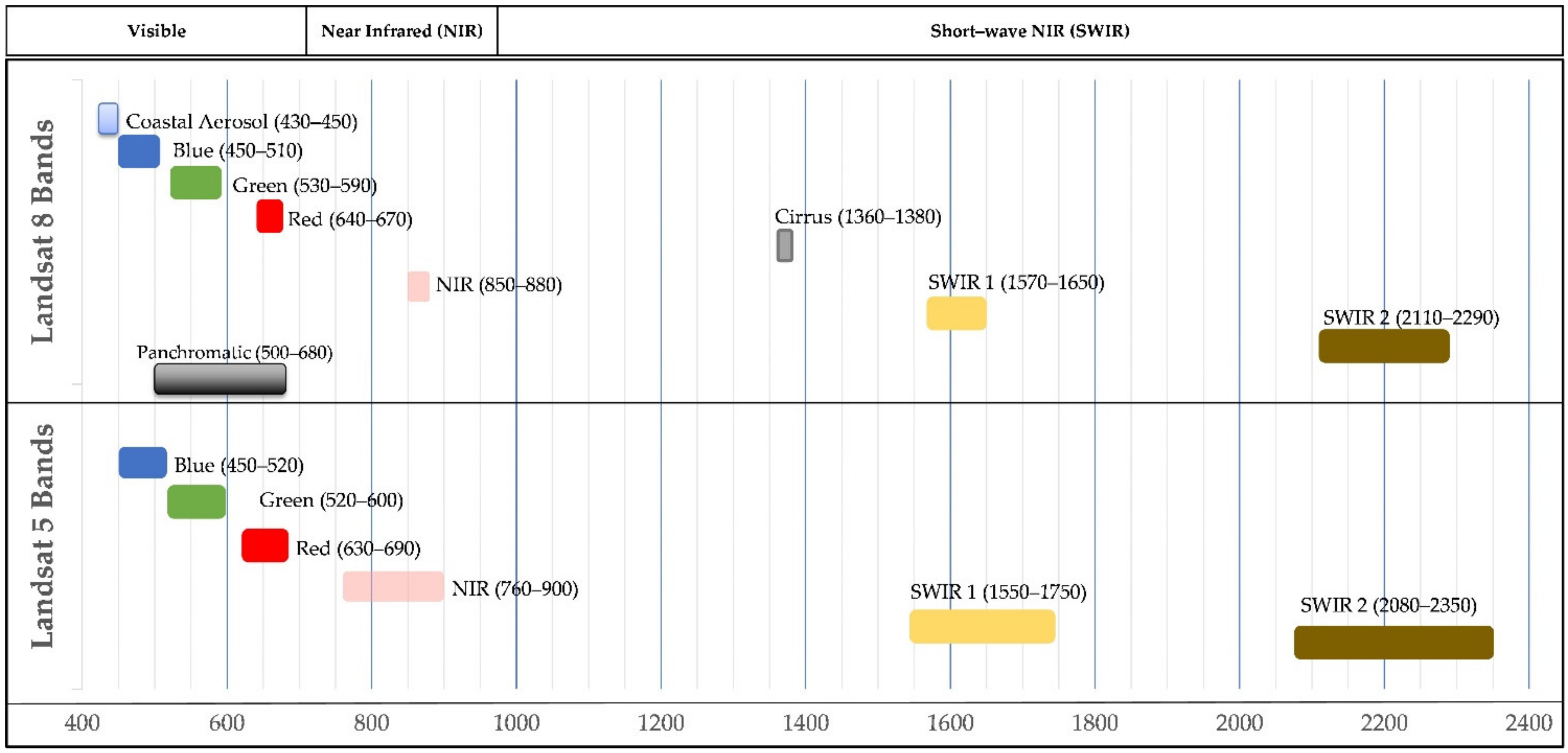
2.2.1. Satellite Data

All the datasets used in this study are available in the Google Earth Engine (GEE) repository. The primary dataset used was the atmospherically corrected, tier 1 surface reflectance Landsat imagery. Landsat 5 was used for the years 2005 and 2010 while Landsat 8 was used for the years 2015 and 2020. Figure 4 shows the multispectral bands of Landsat 5 and 8 data. Operating at a spatial resolution of 30 m, both have a temporal resolution of 16 days. Revolving around in sun-synchronous, near-polar orbit, both data were acquired on the Worldwide Reference System-2 (WRS-2) path/row system.
To acquire smooth continuous coverage of the scene without clouds, we used cloud masking and median filtering functions for the image in GEE, resulting in the annual median composite. In addition to spectral reflectance, different spectral indices (SIs) were derived and added as the input parameters for training. SIs have been used in vegetation studies, especially to assess the health of vegetation, which could provide valuable information in classification approaches. The following were the indices used for our study:
  • Normalized Difference Vegetation Index (NDVI): An indicator of vegetation greenness, NDVI is the ratio of the spectral reflectance difference between the near-infrared (NIR) and red bands to the sum of the reflectances of the Near Infrared (NIR) and red bands [68]:
    NDVI = (NIR − Red)/(NIR + RED),
  • Modified Normalized Difference Water Index (MNDWI): A modified version of the Normalized Difference Water Index, MNDWI enhances the recognition of open water bodies, by removing various noises of built-up areas, soil, and vegetation. It is obtained as the ratio of spectral reflectance difference between the Green and Short-Wave Infrared (SWIR) bands to the sum of the reflectances of the Green and SWIR bands [69]:
    MNDWI = (Green − SWIR1)/(Green + SWIR1),
  • Normalized Difference Built-up Index (NDBI): NDBI is the spectral index to detect built-up areas. It is calculated as normalized difference between Short Wave Infrared (SWIR) and green bands:
    NDBI = (SWIR1 − NIR)/(SWIR1 + NIR),
Topographic information such as slope and elevation were also used in classification. They were derived from the SRTM, which is an international research effort in 2000 to obtain a DEM on a near-global scale. The data in GEE are SRTM V3 product (SRTM Plus) that is provided by NASA JPL at a resolution of 1 arc-second (approximately 30 m) and has undergone a void-filling process using open-source data (ASTER GDEM2, GMTED2010, and NED), as opposed to other versions that contain voids or have been void-filled with commercial sources.
GEE has the Landsat data dating back from its launch to the present day. GEE eases the way in extracting, analyzing, and performing different operations for the earth observed data. Additionally, GEP hosts the historical high-resolution data making it possible to test beforehand for each of the generated reference data for different years.

2.2.2. Reference Data

For generating reference data, unsupervised classification was used as an initial step. Generating a large amount of training data can be tedious. Therefore, unsupervised classification can help understand the distribution of samples and the clustering of similar features. It was applied by Wagle et al. [70] to generate their training data. Thus, we adopted ISO clustering to obtain 100 classes and applied stratified random sampling to generate 800 points. Each point was cross-checked by layering over the high-resolution imagery from GEP of the same year. To have improved representation and accuracy, additional knowledge from the author’s prior knowledge of the study area (hometowns) was applied for the modification, addition, and deletion of points. Based on the ability of clusters and our ability to identify the LC, we generated the following 5 classes: agriculture, built-up, water bodies, forest, and barren (Table 1). These were the most dominant types of LC in the district. Due to the moderate resolution of Landsat, it was not advisable to further subdivide the classes, as it would have been difficult and would result in misclassification.
For the images of 2010 (Landsat 5), a total of 806 reference points for all LC classes were cumulated, while for the images of 2015 (Landsat 8), the number of reference points was expanded to 819. Of the total points, 70% were randomly selected for training and the remaining 30% for validation.

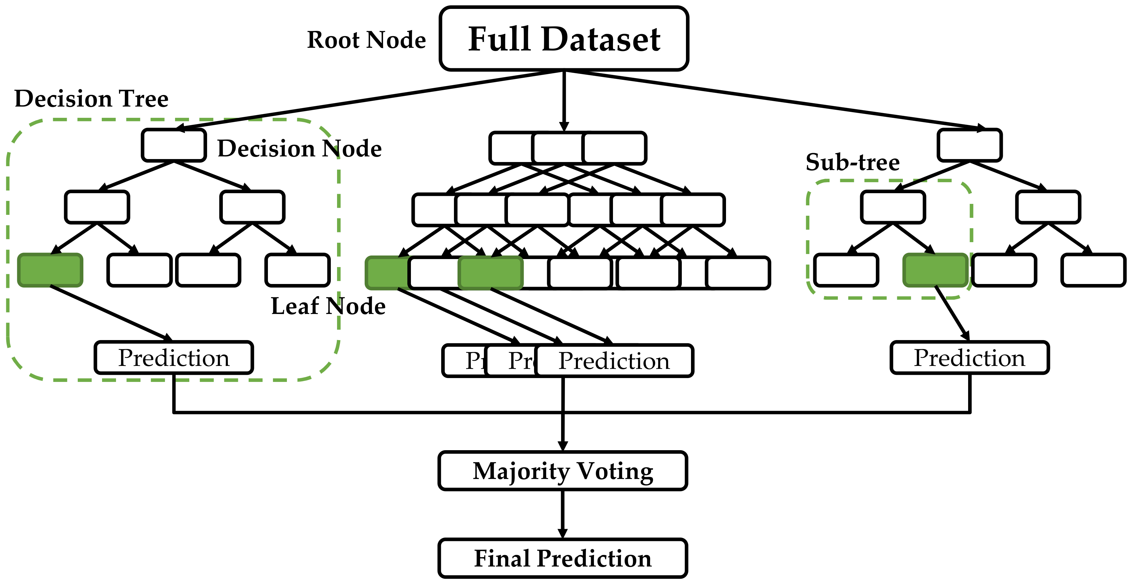
2.2.3. Classification and Accuracy Assessment

Random Forest (RF) is a non-parametric ensemble learning algorithm combining many decision trees, each working independently of the other. It is an improvement on traditional decision trees, and it has been shown to yield better results in numerous case studies. Figure 5 shows the representation of an RF, with decision trees that consist of decision nodes, leaf nodes, and a root node. Each specific decision tree produces the individual output, which is the leaf node of the tree. The final output is chosen using a majority-voting procedure. In this situation, the final output of the system is the output chosen by the majority voting of decision trees.
Decision trees are useful in sorting observations into categories based on features. They aid in differentiating between members of various groups and determining the degree of resemblance among members of the same group. The RF generates a class prediction for each tree, and the class with the highest votes becomes the model’s prediction. RF chooses samples at random with a replacement, resulting in various trees. RF separates a random selection of features, resulting in more variation, as opposed to traditional decision trees, which analyze all potential features and choose the one that creates more variation. RF produces a robust result.
For accuracy assessment, producer’s accuracy (PA), user’s accuracy (UA), overall accuracy (OA), and Kappa statistics (Kappa) were calculated using the 30% validation data via confusion matrix. These statistics were used to evaluate as well as compare the classification results.

2.3. Centre of Gravity

The CoG is the point where the mass of the body seems to be concentrated. In the case of landcover type, it determines the spatial concentration of the landcover. Additionally, the CoG transfer trajectory determines the pattern of landcover change over time and helps in the study of LCC analysis. The concept of an LC CoG is derived from the idea of the population centroid and the economic centroid in geography.
CoG can be calculated as follows:
X t = i = 1 n ( A t i × X i ) i = 1 n X i ,
Y t = i = 1 n ( A t i × Y i ) i = 1 n X i ,
where Xt and Yt are the X and Y coordinates of the CoG of the particular LC in year t, Xi and Yi are the X and Y coordinates of the geometric center of the ith patch, and Ati represents the area of the ith patch.

2.4. Economic Value of Ecosystem Services

Due to the topographical and development stage similarities between China and Nepal, researchers have used a similar coefficient in Nepal for calculating the ESV values in major river basins of Nepal such as the Koshi river basin [71], Gandaki river basin [72], and Karnali river basin [73]. The studies had used the coefficients developed by Xie et al. [74], which had the value zero for built-up areas. Our study also used the same value for agriculture, water bodies, forest, and barren, but used the negative value of built-up areas developed by Duan et al. [75] to address the negative impacts due to growing urban areas, which was also used by Li et al. [59] in their study. The values used are shown in Table 2.
The general formula for the value of ESV is as follows [76]:
ESV = ∑Ai ×Pi,
where ESV is the total ecosystem value (in USD), Ai is the area of land use type i (in hectares), and Pi represents the value coefficient for the ecosystem services provided by land type i (in USD/hectare).

3. Results

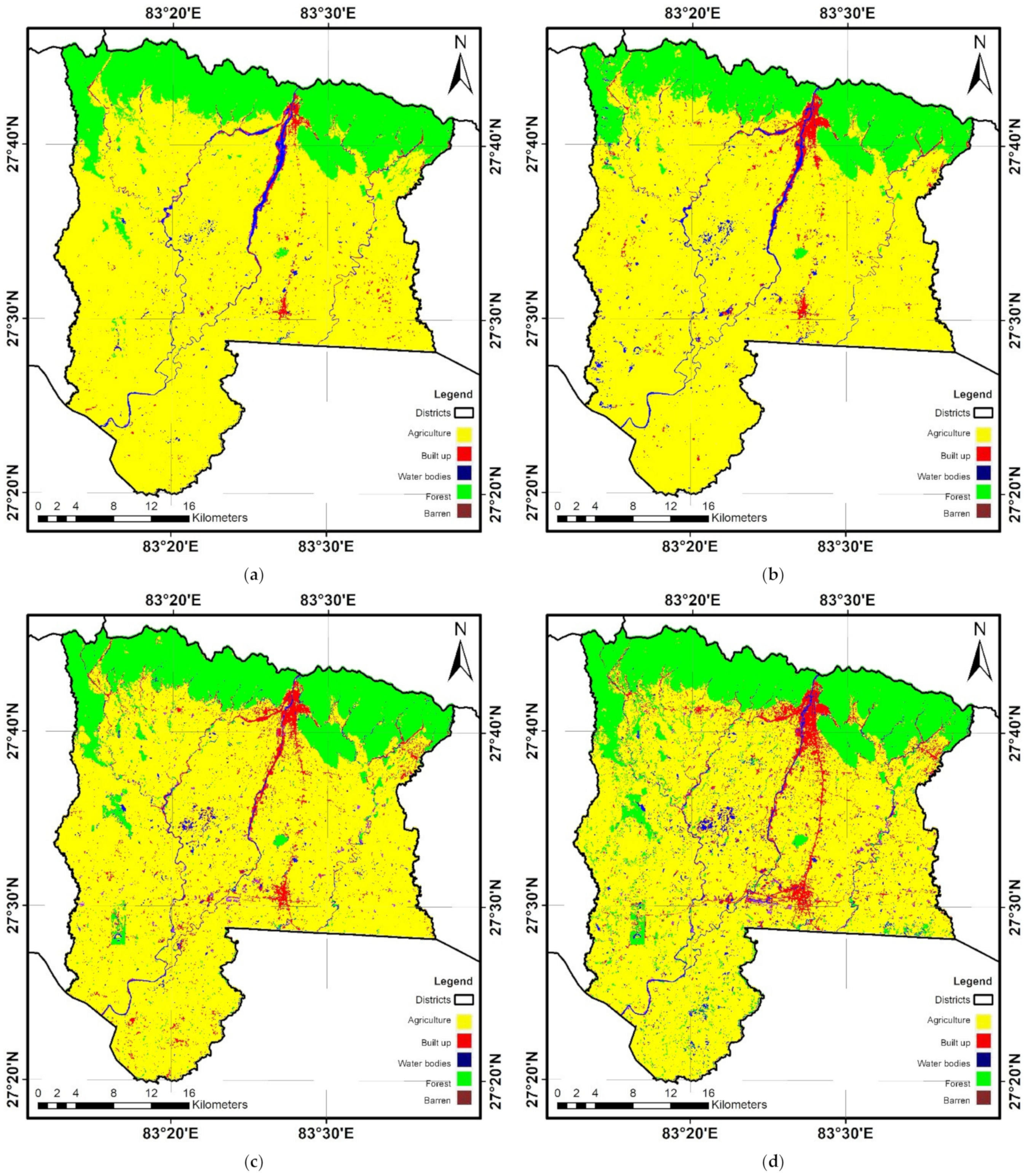
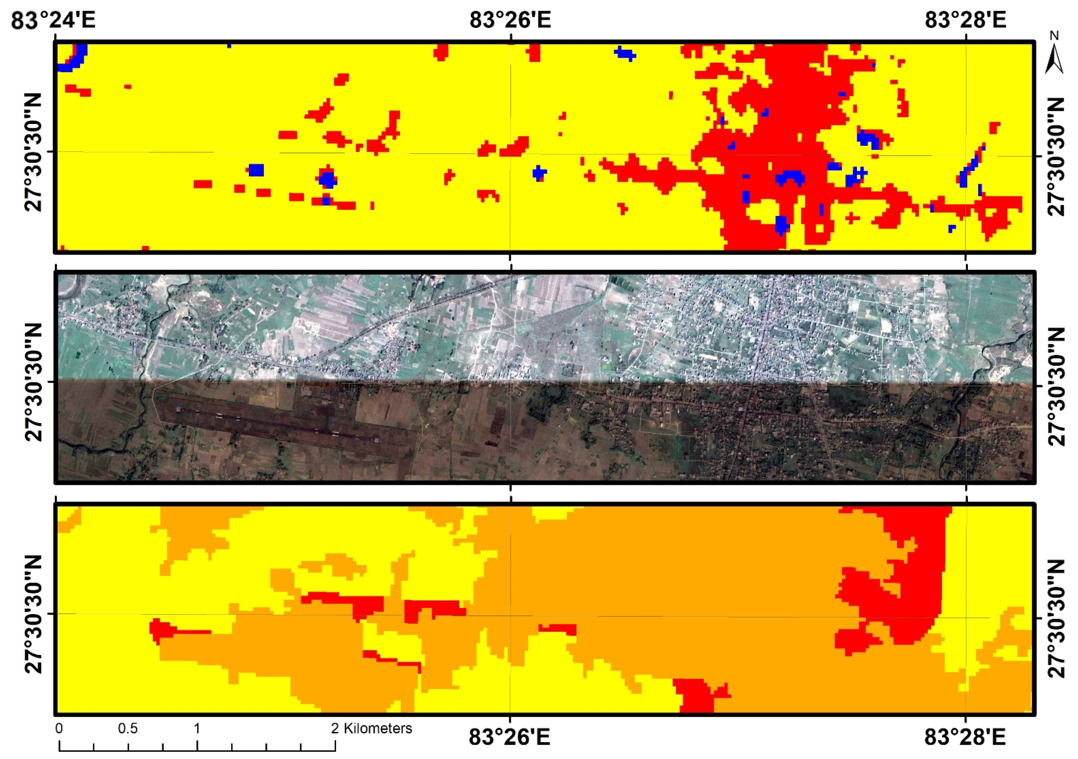
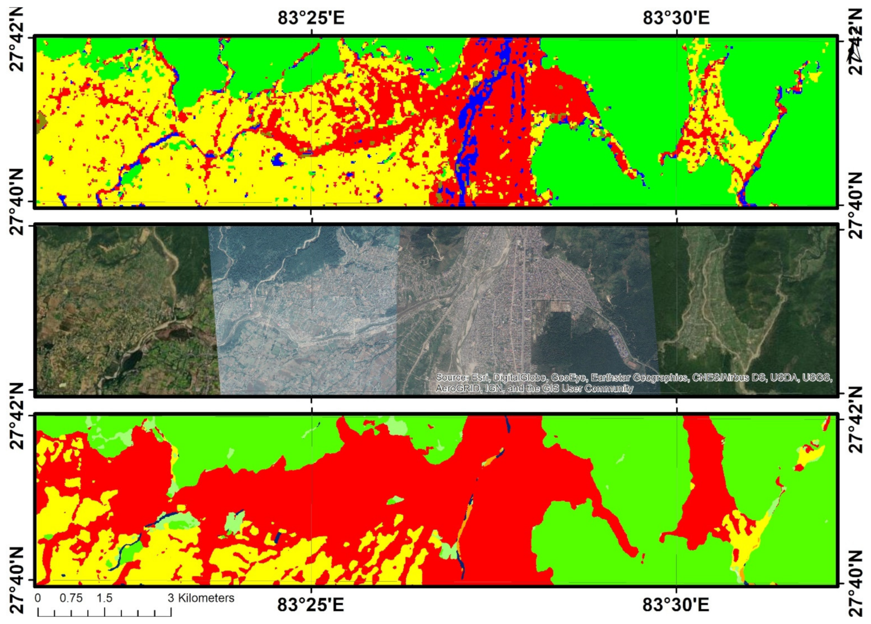
3.1. Land Cover Classification and Accuracy Assessment

The LC maps of the Rupandehi District between the years 2005 and 2020 are shown in Figure 6. The district has seen some great variations and undergone some drastic changes. It can be seen that agricultural lands and forests are among the most abundant classes.
An accuracy assessment was carried out on the resulting classified imagery using the PA, UA, OA, and Kappa from the confusion matrix to test the precision and accuracy of the classified imagery. As the Kappa values greater than 60% are considered as of substantial agreement, it was 62, 66, 68, and 69% for the years 2005, 2010, 2015, and 2020, respectively, showing the good agreement between the classified results and ground truth values in such fragmented LCs. The OA assesses the percentage of data correctly classified. It was found to be the highest (0.80) for 2020 and lowest (0.77) for 2005. For the years 2010 and 2015, it had the same value (0.79). Table 3 shows the accuracy assessment statistics obtained for different years.
To check the correctness of the classification for individual class cover, the PA and UA obtained from the confusion matrix were also calculated. The PA for agriculture remained significantly higher than the other classes for all the years, the lowest being 0.87 for 2005. The UA for agriculture also remained high in comparison to the other classes. It was 0.81 for both 2005 and 2020. The UA and PA for built-up areas were not consistent. It was 0.91 for the year 2010, while for all the other years, it ranged from 0.73 (2005), 0.74 (2020) to 0.76 (2015). The PA was also inconsistent for built-up areas. A significant difference in the performance of the classifier can also be seen in the water class. While the UA remained in the same range, the PA was the lowest (0.27) for the year 2020, but it was 0.75 for 2005 and 2010, and 0.73 for 2015. The forest class was classified accurately to a good extent. The UA for the classification of forest for 2005 was the highest (1) amongst all, and for the other years, it was 0.76 (2005), 0.87 (2010), and 0.95 (2020). The PA for the forest was moderately accurate, 0.86 being the largest value for 2015. The UA and PA for barren land were zero for all the years. This is due to the class imbalance problem. The barren land area is very small in area compared to the other classes, resulting in fewer data for training and testing.
Table 4 shows all the areas of the derived LC maps for the Rupandehi District. While constituting an area of 1003.29 sq. km. (76.9% of the total land) in 2005, the agricultural land has declined to 946.6 sq. km. (72.5%). As compared to other thematic classes, the built-up area has been increasing for each study year. Confined within 18.14 sq. km. in the year 2005, it has increased to an area of 71.15 sq. km., covering 5.45% of the total land area in 2020. The area covered by barren land has been declining as well. Initially, at 2.39 sq. km. for the year 2005, the barren land area was even raised to 2.58 sq. km. in 2015 but has declined since then, standing at 0.65 sq. km. for the year afterward. The area covered by water bodies has greater variations. Covering just 27.26 sq. km. in 2005, it was continuously decreasing for the years 2010 and 2015. However, in 2020, it increased to 23.79 sq. km. Forest cover has been a consistent class. Although the percentage cover has seen fluctuations, there is no drastic change in the cover. The minimum was in 2015 (242.81 sq. km.) and the maximum was in 2010 (266.54 sq. km.).

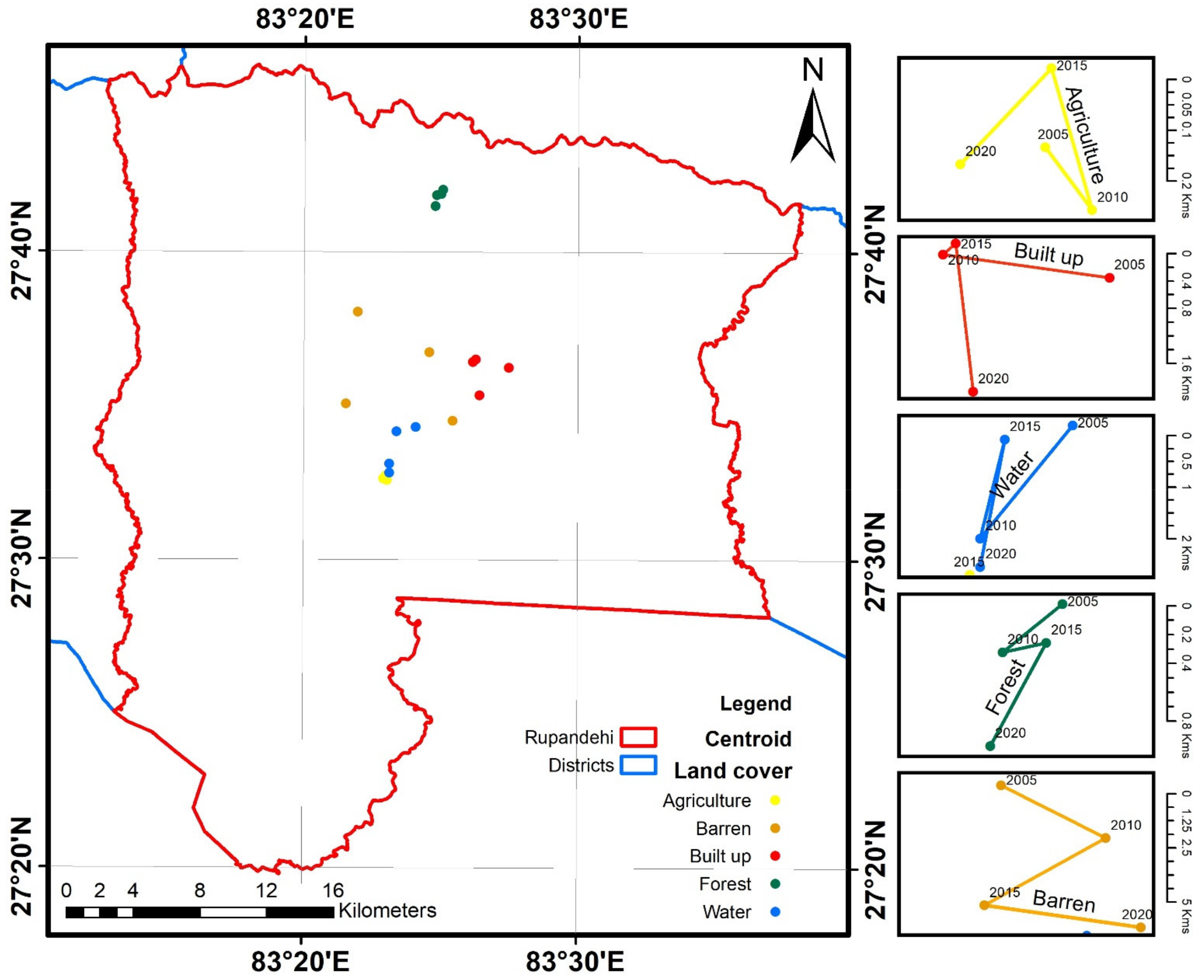
3.2. Analysis of Centre of Gravity

After the preparation of LC maps of different years from 2005 to 2020, we calculated the centroid for each class and mapped the trajectory. The trajectory of the center is the centroid, and their lengths are shown in Figure 7 and Table 5.
Looking at the CoG transfer trajectory of agriculture, we can see that there has not been much change in the spatial pattern of the agricultural land compared to other classes over the past two decades. However, the centroid of agriculture has shifted toward the west, indicating that there was a great migration of people to the western part that started agricultural practices through various means. The transfer trajectory of barren is larger than other classes. There is a zigzag pattern in the trajectory change. From 2005 to 2010, the centroid shifted 4.92 km in the southeast direction. From 2010 to 2015, the centroid shifted around 5.85 km in the southwest direction. Similarly, from 2015 to 2020, the centroid shift was 6.48 km in the southeast direction.
From the CoG transfer trajectory of the built-up area (Figure 7) we can see that there was a huge change in the location from 2005 to 2010 of 2.16 km in a northwest direction, but not much change from 2010 to 2015. Again, from 2015 to 2020, there was a drastic change in the trajectory of 2.16 km towards the south. Overall, the centroid shifted toward the southwest, indicating there was an increase in settlements in the Bhairahawa and western side of the Rupandehi District. There was not much change in the CoG transfer trajectory of Forest. There was a shift of 0.28 km in an eastern direction from 2010 to 2015 and 0.79 km towards the southwest for 2015–2020. The CoG of the water body migrated 2.71 km southwest for 2005–2010, 1.97 km north for 2010–2015, and 2.51 km southwest from 2015–2020. The shift in the centroid in a water body was caused by establishing different artificial ponds for fish farming in the southwestern area. The southwestern part of the Rupandehi District has huge potential for fish farming.

3.3. Ecosystem Value Services Analysis of Land Cover

Based on the value of ecosystem services, modified by Xie et al. [63] and Duan et al. [64] (Table 2), our study used and estimated the ESV between 2005, 2010, 2015, and 2020 in the Rupandehi District, as shown in Table 6.
Among the values of different LULC types, the values of the ecosystem services for agriculture were the highest. It had a value of 701.67 thousand USD in 2005 but fell to 691.31 thousand in 2010, had 7034 thousand USD in 2015, and the lowest value of 662.02 thousand in 2020. With the area covered by built-up increasing, negative values given by built-up areas have become higher. For 2005, it had a negative 15,030 USD, negative 23,200 USD for 2010, negative 34,690 USD for 2015, and negative 58,970 USD for 2020. The values for water bodies have also fluctuated. It was 178.63 thousand USD for 2005. It decreased for both years afterward, with values 124.51 thousand USD for 2010 and a minimum of 94.23 thousand USD for 2015. However, its value rose again to 155.89 thousand USD for 2020.
Forest also has significantly higher values standing at 551.77 thousand USD for 2005, 578.08 thousand USD for 2010, had a slight decline in 2015 with a value of 526.62 thousand USD, and had an increase to 571.02 thousand USD for 2020. Barren land had undergone some serious decline over the recent years. While it increased from 143 thousand USD (2005) to 154 thousand USD (2010), it has since declined to 39 thousand USD for 2015 and remained at the same for 2020 as well. Agriculture, forest, and water bodies comprised the highest, as compared to the other LC types, in 1990.
These fluctuations in class-based ecosystem service value also affected the total ESV. It was highest for the year 2005 with 1417.18 thousand USD but had declined to 1370.85 thousand USD in 2010 and 1289.6 thousand USD in 2015. It had slightly risen to 1330.06 thousand USD in the year 2020.

4. Discussion and Conclusions

This study focused on deriving three major outcomes for the Rupandehi District. Based on the Landsat satellite image, we obtained LC information for the years 2005, 2010, 2015, and 2020 through RF classification in GEE, calculated the CoG for each LC type and analyzed the transfer along the years, and determined the change in ESV over the years. A cloud-based computing platform (GEE) facilitated acquiring and analyzing data for the study, including median composite and derivative indices from Landsat images and topographic information from SRTM DEM. GEE has certainly overcome the tiring effort to download each earth scene and offline analysis. This has reduced the time and cost, increasing efficiency. The study produced satisfactory results in classifying the LC with kappa statistics showing substantial agreement (>0.60) and accuracy in a good range (>0.70) for all the years. We also evaluated the ESV values for individual land cover classes and total values for each of the years, indicating the fluctuations. Lastly, at the end of the paper, we also discuss the aspects and problems of the spatiotemporal analysis of developing regions including the lack of sustainability in the developmental projects.
If we analyze the individual classes, agricultural land, which is the major percentage of LC, has been subjected to various fluctuations. Built-up areas, which were mostly centered in the two major cities, in the earlier years, have now become more spread out, inviting the problems such as land fragmentation and unmanaged urbanization. It increased from 18.14 sq. km. in 2005 to 71.15 km in 2020 (292% increment). A heavy increase in built-up areas can be seen progressing along the highway connecting major cities. Thus, the CoG of a built-up area is located around the centroid of the two cities. The decrease in water bodies from 2005 to 2015 can be explained by riverside encroachment and drying up of natural ponds due to extreme heat. However, artificial ponds for commercial fish farming have increased over the past few years, which can explain the increase in area in 2020 in a western direction. Forest area is subjected to less change in compared to other classes. It may also be the undisturbed class as the shift in the CoG is also very low. Strict rules against deforestation and the concept of community forest may be the reasons for the increasing forest area. In 2015, significant changes can be seen with decreasing forest and water bodies and increasing agriculture. The conversion of private green covers into farmland may be a contributing factor for that. Barren land increased from 2005 to 2010 and then, subsequently, decreased in the following years. This may be explained by the riverbank encroachment due to the human settlement. The barren lands in our study are generally the shores of rivers and ponds. The patches are often thin and elongated along with the water sources. Due to the limited spatial resolution of Landsat, the area of the barren land was smaller than the individual pixel most of the time, resulting in either water bodies or nearby major classes. Thus, it generated 0 values for the UA and the PA. The year 2005 had the highest ESV value due to the large area of ecological land (agriculture, water bodies, and forest). As the ESV values are directly proportional to the area of the land cover, increasing the built-up area increased negative ESVs. Due to the fluctuations in the area of other land cover classes, ESV values were also varied over the years.
We also compared our classification results of 2010 with a national LC map prepared by Integrated Mountain Development (ICIMOD) [61]. ICIMOD had divided the land into 12 classes and used object-based classification, and obtained a little higher overall accuracy compared to ours, of 85.13%, and a kappa of 0.82. Figure 8 shows the comparison of our result with that of ICIMOD, alongside high-resolution imagery from GEP for 2010. The comparison is performed by zooming in on Bhairahawa, the second-largest city in the district. While the ICIMOD landcover helps to identify the runway in the airport, our results just show certain signs of a built-up area. Both studies have identified agriculture to a quite good extent. However, our classification showed better results in identifying the water bodies and overall built-up areas, which is shown mostly as barren in the work by ICIMOD. Due to the inclusion of broad classes, ICIMOD, thus, had the advantage of identifying the peri-urban areas but had the limitation of misclassifying the major classes.
For the year 2020, we compared our classified LC map with a global 10-meter resolution map of the Earth’s land surface produced by ESRI, alongside high-resolution imagery from GEP for the same year. ESRI had produced the classification results with 10 classes processing over 400,000 Earth observations. Figure 9 shows the comparison between them focused at Butwal, the biggest city of the district. The classes were more generalized by ESRI, giving the smoothness, but failed to quantify the minor classes such as water bodies. It can be seen that water bodies were more accurately classified in our work compared to ESRI’s LC. Similarly, the problem of the fragmentation of agricultural lands by haphazard built-up areas was observed more clearly in our work.
From the results of our study, we can discuss the following aspects of the spatiotemporal changes in developing regions:
  • Sustainability is something every developmental effort should focus on. However, Nepal is often struggling to incorporate this into its strategies. District-level policies also lag in that aspect. Providing the historical and present status of LC can help in understanding how the land resources have been used over the years. The critical information obtained can be of high importance for planning more sustainably. It is highly recommended to incorporate ecological-based approaches to address disturbances in the ecosystem in the short- and long-term regulations. It must be ensured that the concepts of open spaces, green fuels, water conservation, forest restoration, food production, and watershed management are given high importance to curb the unplanned and haphazard development.
  • Along with knowing the status of LC, it is extremely crucial to monitor where the particular LC class is focused. The analysis of the central displacement of LC can help understand the development of the region and provide references for resource management and territorial planning. The rapid shift of a particular LC in a direction can be an alarm to the overexploitation of another resource. Therefore, the analysis of LC along with the gravity shift of the classes is endorsed.
  • Calculating ESV is a definitive and appropriate approach for evaluating the ecosystem on a monetary basis providing the scientific ground for commanding the policies. In addition, ESV can be an effective way of communicating the results. It can provide insights into the load that we put on ecosystems and thus can help in implementing proper plans and strategies by district administration offices and local governmental bodies to stop the exploitation of resources. Integrating economic, ecological, and social dimensions in spatial planning ensures sustainable urban development plans.
  • Accuracy is highly dependent on the quality of LC data and the unit value of ESV for each LC class type. Therefore, the improvement in LC data is highly recommended, along with more details and empirical studies for obtaining a unit value of ecosystem services.
  • Studies such as ours are scientific efforts for developing regions, incorporating spatial econometrics and statistics with earth observation studies and GIS. Often, the topics are left out at the local level and are not considered in urban planning and development.
The study is the first of its kind in the Rupandehi District. The pattern and above discussion would be helpful to concerned authorities and stakeholders. We hope the study could be fruitful to the authorities interested in knowing the spatial changes of the land cover and also to those working on maintaining sustainable ecosystem services. Besides our effort to quantify the spatiotemporal analysis of the region, this study faced some challenges and limitations, which are as follows:
  • Stakeholders may be interested in the extraction of small classes such as road networks, types of forest, grassland, or pasture, which this study did not try to achieve due to the mid resolution of Landsat and the fragmented characteristics of the study area. Additionally, it can only be possible with a high level of spatial data. However, it may be difficult to acquire high-resolution images for long-term studies.
  • Another problem is the class imbalance problem. While we had enough training, data were labeled as agriculture due to the large area covered by farmland, but the minority classes such as barren land and water bodies faced the problem of insufficient training data in comparison to the majority classes. However, we compensated for the problem by manually adding the points for the minority classes.
  • Obtaining a proper ESV is difficult to obtain in the context of Nepal. We used the values derived from the Tibetan plateau, which shares a border with Nepal and has a similar economic and development stage. The values have also been used by previous researchers in the context of Nepal. However, there is certainly the need for detailed and thoroughly established ESV coefficients applicable to the whole of Nepal.
Future work can focus on resolving the limitations considering the new data, techniques, and coefficients. Either classifying more LC classes on Landsat or applying data fusion techniques with Sentinel imagery could be conducted to obtain finer and more precise LC classes. The class imbalance problem can be addressed using resampling techniques (either an under-sample majority class or an oversample minority class). Trying a variety of algorithms can be beneficial with imbalanced datasets. Besides RF, ensemble methods such as boosting, and bagging could be implemented to evaluate accuracy and robustness. For improvement in regional-based ESV factors, local and federal level collaborative research is recommended along with the inclusion of questionnaires for local ecologists and community-based surveys in the method.

Author Contributions

Conceptualization, Aman KC and Tri Dev Acharya; data curation, Aman KC and Nimisha Wagle; formal analysis, Aman KC and Tri Dev Acharya; investigation, Nimisha Wagle; methodology, Aman KC, Nimisha Wagle and Tri Dev Acharya; resources, Tri Dev Acharya; software, Nimisha Wagle; supervision, Tri Dev Acharya; validation, Nimisha Wagle; visualization, Tri Dev Acharya; writing—original draft, Aman KC; writing—review and editing, Nimisha Wagle and Tri Dev Acharya. All authors have read and agreed to the published version of the manuscript.

Funding

This research received no external funding.

Institutional Review Board Statement

Not applicable.

Informed Consent Statement

Not applicable.

Data Availability Statement

All data are available in Google Earth Engine Data Catalogue. For code and training data visit https://github.com/wagle1996/Landcover-mapping-CoG-ESV.

Acknowledgments

We acknowledge the free availability of data via USGS and GEE. The work is a result of the #Mentor4Nepal Initiative (https://github.com/trydave/Mentor4Nepal), which supports recent graduates and early career professionals focusing on the enhancement of one’s skill set, support for a research project, and a collaborative publication. The authors would also like to thank three anonymous reviewers for their time and effort to provide constructive comments and suggestions and thus improving the original manuscript.

Conflicts of Interest

The authors declare no conflict of interest.

References

  1. Liu, L.; Zhang, X.; Gao, Y.; Chen, X.; Shuai, X.; Mi, J. Finer-Resolution Mapping of Global Land Cover: Recent Developments, Consistency Analysis, and Prospects. J. Remote Sens. 2021, 2021, 1–38. [Google Scholar] [CrossRef]
  2. Ban, Y.; Gong, P.; Giri, C. Global land cover mapping using Earth observation satellite data: Recent progresses and challenges. ISPRS J. Photogramm. Remote Sens. 2015, 103, 1–6. [Google Scholar] [CrossRef] [Green Version]
  3. Ministry of Forest and Environment National Level Forests and Land Cover Analysis of Nepal using Google Earth Images. Kathmandu. 2019. Available online: http://frtc.gov.np/old/downloadfile/Forest%20and%20Land%20Cover%20Analysis_final_report_1550056440.pdf (accessed on 2 August 2021).
  4. Verburg, P.H.; Neumann, K.; Nol, L. Challenges in using land use and land cover data for global change studies. Glob. Chang. Biol. 2011, 17, 974–989. [Google Scholar] [CrossRef] [Green Version]
  5. Moody, A.; Woodcock, C.E. Scale-dependent errors in the estimation of land-cover proportions: Implications for global land-cover datasets. Photogramm. Eng. Remote Sens. 1994, 60, 585–594. [Google Scholar]
  6. Gong, P.; Liu, H.; Zhang, M.; Li, C.; Wang, J.; Huang, H.; Clinton, N.; Ji, L.; Li, W.; Bai, Y.; et al. Stable classification with limited sample: Transferring a 30-m resolution sample set collected in 2015 to mapping 10-m resolution global land cover in 2017. Sci. Bull. 2019, 64, 370–373. [Google Scholar] [CrossRef] [Green Version]
  7. Hansen, M.C.; Potapov, P.V.; Moore, R.; Hancher, M.; Turubanova, S.A.; Tyukavina, A.; Thau, D.; Stehman, S.V.; Goetz, S.J.; Loveland, T.R.; et al. High-Resolution Global Maps of 21st-Century Forest Cover Change. Science 2013, 342, 850–853. [Google Scholar] [CrossRef] [Green Version]
  8. ESA Land Cover CCI: Product User Guide. Available online: http://maps.elie.ucl.ac.be/CCI/viewer/download/ESACCI-LC-Ph2-PUGv2_2.0.pdf (accessed on 3 June 2021).
  9. Defourny, P.; Vancutsem, C.; Bicheron, C.; Brockmann, C.; Nino, F.; Schouten, L.; Leroy, M. GlobCover: A 300M Global Land Cover Product for 2005 Using ENVISAT MERIS Time Series. In Proceedings of the ISPRS Commission VII Mid-Term Symposium: Remote Sensing: From Pixels to Processes, Enschede, The Netherlands, 8–11 May 2006; pp. 8–11. [Google Scholar]
  10. Falls, S.; Loveland, T.; Reed, B.; Brown, J.; Ohlen, D.; Zhu, Z.; Yang, L.; Merchant, J. Development of a global land cover characteristics database and IGBP DISCover from 1 km AVHRR data. Int. J. Remote Sens. 2000, 21, 1303–1330. [Google Scholar]
  11. Friedl, M.A.; Sulla-Menashe, D.; Tan, B.; Schneider, A.; Ramankutty, N.; Sibley, A.; Huang, X. MODIS Collection 5 global land cover: Algorithm refinements and characterization of new datasets. Remote Sens. Environ. 2010, 114, 168–182. [Google Scholar] [CrossRef]
  12. Liu, H.; Gong, P.; Wang, J.; Clinton, N.; Bai, Y.; Liang, S. Annual dynamics of global land cover and its long-term changes from 1982 to 2015. Earth Syst. Sci. Data 2020, 12, 1217–1243. [Google Scholar] [CrossRef]
  13. Gong, P.; Wang, J.; Yu, L.; Zhao, Y.; Zhao, Y.; Liang, L.; Niu, Z.; Huang, X.; Fu, H.; Liu, S.; et al. Finer resolution observation and monitoring of global land cover: First mapping results with Landsat TM and ETM+ data. Int. J. Remote Sens. 2013, 34, 2607–2654. [Google Scholar] [CrossRef] [Green Version]
  14. Karra, K.; Kontgis, C.; Statman-Weil, Z.; Mazzariello, J.; Mathis, M.; Brumby, S. Global land use/land cover with Sentinel-2 and deep learning. In Proceedings of the IGARSS 2021-2021 IEEE International Geoscience and Remote Sensing Symposium, Brussels, Belgium, 12–16 July 2021. [Google Scholar]
  15. Li, J.; Zheng, X.; Zhang, C.; Chen, Y. Impact of land-use and land-cover change on meteorology in the Beijing-Tianjin-Hebei region from 1990 to 2010. Sustainability 2018, 10, 176. [Google Scholar] [CrossRef] [Green Version]
  16. Acharya, T.D.; Parajuli, J.; Shahi, K.; Poudel, D.; Yang, I. Extraction and Modelling of Spatio-Temporal Urban Change in Kathmandu Valley. Int. J. IT Eng. Appl. Sci. Res. 2015, 4, 1–11. [Google Scholar]
  17. Wang, S.W.; Gebru, B.M.; Lamchin, M.; Kayastha, R.B.; Lee, W.K. Land Use and Land Cover Change Detection and Prediction in the Kathmandu District of Nepal Using Remote Sensing and GIS. Sustainability 2020, 12, 3925. [Google Scholar] [CrossRef]
  18. Kaplan, G.; Avdan, U.; Avdan, Z.Y. Urban Heat Island Analysis Using the Landsat 8 Satellite Data: A Case Study in Skopje, Macedonia. Proceedings 2018, 2, 358. [Google Scholar] [CrossRef] [Green Version]
  19. Cao, F.; Dan, L.; Ma, Z.; Gao, T. The impact of land use and land cover change on regional climate over East Asia during 1980–2010 using a coupled model. Theor. Appl. Climatol. 2021, 145, 549–565. [Google Scholar] [CrossRef]
  20. Pekel, J.-F.; Cottam, A.; Gorelick, N.; Belward, A.S. High-resolution mapping of global surface water and its long-term changes. Nature 2016, 540, 418–422. [Google Scholar] [CrossRef] [PubMed]
  21. Hansen, M.C.; Sohlberg, R.; Defries, R.S.; Townshend, J.R.G. Global land cover classification at 1 km spatial resolution using a classification tree approach. Int. J. Remote Sens. 2000, 21, 1331–1364. [Google Scholar] [CrossRef]
  22. Haro-Carrión, X.; Southworth, J. Understanding land cover change in a fragmented forest landscape in a biodiversity hotspot of coastal Ecuador. Remote Sens. 2018, 10, 1980. [Google Scholar] [CrossRef] [Green Version]
  23. Nakalembe, C.; Becker-Reshef, I.; Bonifacio, R.; Hu, G.; Humber, M.L.; Justice, C.J.; Keniston, J.; Mwangi, K.; Rembold, F.; Shukla, S.; et al. A review of satellite-based global agricultural monitoring systems available for Africa. Glob. Food Sec. 2021, 29, 100543. [Google Scholar] [CrossRef]
  24. Acharya, T.D.; Yang, I.T.; Lee, D.H. Land cover classification of imagery from Landsat operational land imager based on optimum index factor. Sens. Mater. 2018, 30, 1753–1764. [Google Scholar] [CrossRef]
  25. Lee, J.K.; Acharya, T.D.; Lee, D.H. Exploring land cover classification accuracy of Landsat 8 image using spectral index layer stacking in hilly region of South Korea. Sens. Mater. 2018, 30, 2927–2941. [Google Scholar] [CrossRef]
  26. Huguenin, R.L.; Karaska, M.A.; Van Blaricom, D.; Jensen, J.R. Subpixel Classification of Bald Cypress and Tupelo Gum Trees in Thematic Mapper Imagery. Photogramm. Eng. Remote Sens. 1997, 63, 717–725. [Google Scholar]
  27. Li, M.; Zang, S.; Zhang, B.; Li, S.; Wu, C. A Review of Remote Sensing Image Classification Techniques: The Role of Spatio-contextual Information. Eur. J. Remote Sens. 2014, 47, 389–411. [Google Scholar] [CrossRef]
  28. Zhang, J.; Kerekes, J. Unsupervised Urban Land-Cover Classification Using WorldView-2 Data and Self-Organizing Maps. Available online: https://www.researchgate.net/publication/224263092_Unsupervised_urban_land-cover_classification_using_WorldView-2_data_and_self-organizing_maps (accessed on 3 July 2021).
  29. Mishra, A.; Karwariya, S.; Goyal, S. Land use/Land cover Mapping of Chhatarpur District, Madhya Pradesh, India Using Unsupervised Classification Technique. IOSR J. Eng. 2012, 2, 51–56. [Google Scholar] [CrossRef]
  30. Chen, Q.; Kuang, G.; Li, J.; Sui, L.; Li, D. Unsupervised land cover/land use classification using PolSAR imagery based on scattering similarity. IEEE Trans. Geosci. Remote Sens. 2013, 51, 1817–1825. [Google Scholar] [CrossRef]
  31. GISGeograpy Image Classification Techniques in Remote Sensing. Available online: http://gisgeography.com/image-classification-techniques-remote-sensing/ (accessed on 3 July 2021).
  32. Verbeiren, S.; Eerens, H.; Piccard, I.; Bauwens, I.; Van Orshoven, J. Sub-pixel classification of SPOT-VEGETATION time series for the assessment of regional crop areas in Belgium. Int. J. Appl. Earth Obs. Geoinf. 2008, 10, 486–497. [Google Scholar] [CrossRef]
  33. Toure, S.I.; Stow, D.A.; Shih, H.C.; Weeks, J.; Lopez-Carr, D. Land cover and land use change analysis using multi-spatial resolution data and object-based image analysis. Remote Sens. Environ. 2018, 210, 259–268. [Google Scholar] [CrossRef]
  34. Gao, Y.; Mas, J.F.; Niemeyer, I.; Marpu, P.R.; Palacio, J.L. Object-based image analysis for mapping land-cover in a forest area. In Proceedings of the 5th International Symposium: Spatial Data Quality, Enschede, The Netherlands, 13–15 June 2007; pp. 13–15. [Google Scholar]
  35. Kim, H.-O.; Yeom, J.-M. A Study on Object-Based Image Analysis Methods for Land Cover Classification in Agricultural Areas. J. Korean Assoc. Geogr. Inf. Stud. 2012, 15, 26–41. [Google Scholar] [CrossRef] [Green Version]
  36. Stephens, D.; Diesing, M. A Comparison of Supervised Classification Methods for the Prediction of Substrate Type Using Multibeam Acoustic and Legacy Grain-Size Data. PLoS ONE 2014, 9, e93950. [Google Scholar] [CrossRef]
  37. Breiman, L. Random Forests. Mach. Learn. 2001, 45, 5–32. [Google Scholar] [CrossRef] [Green Version]
  38. Gislason, P.O.; Benediktsson, J.A.; Sveinsson, J.R. Random Forests for land cover classification. Pattern Recognit. Lett. 2006, 27, 294–300. [Google Scholar] [CrossRef]
  39. Eisavi, V.; Homayouni, S.; Yazdi, A.M.; Alimohammadi, A. Land cover mapping based on random forest classification of multitemporal spectral and thermal images. Environ. Monit. Assess. 2015, 187, 1–14. [Google Scholar] [CrossRef] [PubMed]
  40. Kolli, M.K.; Opp, C.; Karthe, D.; Groll, M. Mapping of Major Land-Use Changes in the Kolleru Lake Freshwater Ecosystem by Using Landsat Satellite Images in Google Earth Engine. Water 2020, 12, 2493. [Google Scholar] [CrossRef]
  41. Al Mamun, A. Identification and Monitoring the Change of Land Use Pattern Using Remote Sensing and GIS: A Case Study of Dhaka City. IOSR J. Mech. Civ. Eng. 2013, 6, 20–28. [Google Scholar] [CrossRef]
  42. Sidhu, N.; Pebesma, E.; Câmara, G. Using Google Earth Engine to detect land cover change: Singapore as a use case. Eur. J. Remote Sens. 2018, 51, 486–500. [Google Scholar] [CrossRef]
  43. Liu, C.; Li, W.; Zhu, G.; Zhou, H.; Yan, H.; Xue, P. Land Use/Land Cover Changes and Their Driving Factors in the Northeastern Tibetan Plateau Based on Geographical Detectors and Google Earth Engine: A Case Study in Gannan Prefecture. Remote Sens. 2020, 12, 3139. [Google Scholar] [CrossRef]
  44. Huang, H.; Chen, Y.; Clinton, N.; Wang, J.; Wang, X.; Liu, C.; Gong, P.; Yang, J.; Bai, Y.; Zheng, Y.; et al. Mapping major land cover dynamics in Beijing using all Landsat images in Google Earth Engine. Remote Sens. Environ. 2017, 202, 166–176. [Google Scholar] [CrossRef]
  45. Zhang, D.-D.; Zhang, L. Land Cover Change in the Central Region of the Lower Yangtze River Based on Landsat Imagery and the Google Earth Engine: A Case Study in Nanjing, China. Sensors 2020, 20, 2091. [Google Scholar] [CrossRef] [Green Version]
  46. Venkatappa, M.; Sasaki, N.; Shrestha, R.P.; Tripathi, N.K.; Ma, H.-O. Determination of Vegetation Thresholds for Assessing Land Use and Land Use Changes in Cambodia using the Google Earth Engine Cloud-Computing Platform. Remote Sens. 2019, 11, 1514. [Google Scholar] [CrossRef] [Green Version]
  47. Li, A.; Lei, G.; Cao, X.; Zhao, W.; Deng, W.; Koirala, H.L. Land Cover Change and Its Driving Forces in Nepal Since 1990. In Land Cover Change and Its Eco-Environmental Responses in Nepal; Springer: Singapore, 2017; pp. 41–65. ISBN 9789811028908. [Google Scholar]
  48. Hu, Y.; Hu, Y. Land Cover Changes and Their Driving Mechanisms in Central Asia from 2001 to 2017 Supported by Google Earth Engine. Remote Sens. 2019, 11, 554. [Google Scholar] [CrossRef] [Green Version]
  49. Shafizadeh-Moghadam, H.; Khazaei, M.; Alavipanah, S.K.; Weng, Q. Google Earth Engine for large-scale land use and land cover mapping: An object-based classification approach using spectral, textural and topographical factors. GISci. Remote Sens. 2021, 58, 914–928. [Google Scholar] [CrossRef]
  50. Xie, S.; Liu, L.; Zhang, X.; Yang, J.; Chen, X.; Gao, Y. Automatic Land-Cover Mapping using Landsat Time-Series Data based on Google Earth Engine. Remote Sens. 2019, 11, 3023. [Google Scholar] [CrossRef] [Green Version]
  51. Chen, H.; Chen, C. Transfer analysis of land-use type gravity center based on Landsat data—A case study of Zhoushan, China. IOP Conf. Ser. Earth Environ. Sci. 2021, 658, 012035. [Google Scholar] [CrossRef]
  52. Li, Z.; Jiang, W.; Wang, W.; Lei, X.; Deng, Y. Exploring spatial-temporal change and gravity center movement of construction land in the Chang-Zhu-Tan urban agglomeration. J. Geogr. Sci. 2019, 29, 1363–1380. [Google Scholar] [CrossRef] [Green Version]
  53. Li, Z.; Luan, W.; Zhang, Z.; Su, M. Relationship between urban construction land expansion and population/economic growth in Liaoning Province, China. Land Use Policy 2020, 99, 105022. [Google Scholar] [CrossRef]
  54. Costanza, R.; D’Arge, R.; de Groot, R.; Farber, S.; Grasso, M.; Hannon, B.; Limburg, K.; Naeem, S.; O’Neill, R.V.; Paruelo, J.; et al. The value of the world’s ecosystem services and natural capital. Nature 1997, 387, 253–260. [Google Scholar] [CrossRef]
  55. Gee, K.; Burkhard, B. Cultural ecosystem services in the context of offshore wind farming: A case study from the west coast of Schleswig-Holstein. Ecol. Complex. 2010, 7, 349–358. [Google Scholar] [CrossRef]
  56. Huang, X.; Chen, Y.; Ma, J.; Chen, Y. Study on change in value of ecosystem service function of Tarim River. Acta Ecol. Sin. 2010, 30, 67–75. [Google Scholar] [CrossRef]
  57. Kreuter, U.P.; Harris, H.G.; Matlock, M.D.; Lacey, R.E. Change in ecosystem service values in the San Antonio area, Texas. Ecol. Econ. 2001, 39, 333–346. [Google Scholar] [CrossRef]
  58. Tong, C.; Feagin, R.A.; Lu, J.; Zhang, X.; Zhu, X.; Wang, W.; He, W. Ecosystem service values and restoration in the urban Sanyang wetland of Wenzhou, China. Ecol. Eng. 2007, 29, 249–258. [Google Scholar] [CrossRef]
  59. Li, F.; Ye, Y.P.; Song, B.W.; Wang, R.S.; Tao, Y. Assessing the changes in land use and ecosystem services in Changzhou municipality, Peoples’ Republic of China, 1991–2006. Ecol. Indic. 2014, 42, 95–103. [Google Scholar] [CrossRef]
  60. Ramsar Convention Secretariat Wetlands—World’s Most Valuable Ecosystem—Disappearing Three Times Faster than Forests, Warns New Report. Available online: https://www.ramsar.org/news/wetlands-worlds-most-valuable-ecosystem-disappearing-three-times-faster-than-forests-warns-new (accessed on 29 July 2021).
  61. Uddin, K.; Shrestha, H.L.; Murthy, M.S.R.; Bajracharya, B.; Shrestha, B.; Gilani, H.; Pradhan, S.; Dangol, B. Development of 2010 national land cover database for the Nepal. J. Environ. Manag. 2015, 148, 82–90. [Google Scholar] [CrossRef]
  62. Bakrania, S. Urbanisation and Urban Growth in Nepal; (GSDRC Helpdesk Research Report 1294); GSDRC, University of Birmingham: Birmingham, UK, 2015. [Google Scholar]
  63. Muzzini, E.; Aparicio, G. Urban Growth and Spatial Transition in Nepal; The World Bank: Washington, DC, USA, 2013; ISBN 978-0-8213-9659-9. [Google Scholar]
  64. Dhakal, B. Statistical trend and spatial patterns of urbanization in Nepal. Int. Res. J. Nat. Appl. Sci. 2015, 2, 98–110. [Google Scholar]
  65. Central Bureau of Statistics. Statistical Bulletin 2011/12, Vol. 105, No. 1; Central Bureau of Statistics: Kathmandu, Nepal, 2011. [Google Scholar]
  66. United States Geological Survey USGS Landsat Missions-Landsat 5. Available online: https://www.usgs.gov/core-science-systems/nli/landsat/landsat-5?qt-science_support_page_related_con=0#qt-science_support_page_related_con (accessed on 23 July 2021).
  67. United States Geological Survey USGS Landsat Missions-Landsat 8. Available online: https://www.usgs.gov/core-science-systems/nli/landsat/landsat-8?qt-science_support_page_related_con=0#qt-science_support_page_related_con (accessed on 23 July 2021).
  68. KC, A.; Acharya, T.D.; Wagle, N.; Lee, D.H. Tracking Long-term Phenological Shift in Response to Climatic Parameters in Chitwan National Park, Nepal. Sens. Mater. 2021, 33. [Google Scholar] [CrossRef]
  69. Xu, H. Modification of normalised difference water index (NDWI) to enhance open water features in remotely sensed imagery. Int. J. Remote Sens. 2006, 27, 3025–3033. [Google Scholar] [CrossRef]
  70. Wagle, N.; Acharya, T.D.; Kolluru, V.; Huang, H.; Lee, D.H. Multi-Temporal Land Cover Change Mapping Using Google Earth Engine and Ensemble Learning Methods. Appl. Sci. 2020, 10, 8083. [Google Scholar] [CrossRef]
  71. Zhilong, Z.; Xue, W.; Yili, Z.; Jungang, G. Assessment of Changes in the Value of Ecosystem Services in the Koshi River Basin, Central High Himalayas Based on Land Cover Changes and the CA-Markov Model. J. Resour. Ecol. 2017, 8, 67–76. [Google Scholar] [CrossRef]
  72. Rai, R.; Zhang, Y.; Paudel, B.; Acharya, B.K.; Basnet, L. Land Use and Land Cover Dynamics and Assessing the Ecosystem Service Values in the Trans-Boundary Gandaki River Basin, Central Himalayas. Sustainability 2018, 10, 3052. [Google Scholar] [CrossRef] [Green Version]
  73. Shrestha, B.; Ye, Q.; Khadka, N. Assessment of Ecosystem Services Value Based on Land Use and Land Cover Changes in the Transboundary Karnali River Basin, Central Himalayas. Sustainability 2019, 11, 3183. [Google Scholar] [CrossRef] [Green Version]
  74. Xie, G.D.; Lu, C.X.; Leng, Y.F.; Zheng, D.U.; Li, S.C. Ecological assets valuation of the Tibetan Plateau. J. Nat. Resour. 2003, 18, 189–196. [Google Scholar] [CrossRef]
  75. Duan, R.J.; Hao, J.M.; Wang, J. Study on changes of land-use structure and eco-service function value—A case study for Datong, Shanxi Province. Ecol. Econ. 2005, 3, 60–64. [Google Scholar]
  76. Zhao, H.; Xie, F.; Cao, M.; Wei, W.; Wang, H.; Zhao, M. Dynamic evaluation of ecosystem service value in southern mountainous areas of Jinan based on 3 “s” technology. E3S Web Conf. 2019, 118, 04007. [Google Scholar] [CrossRef]
Figure 1. Area of urban center in different geographical regions of Nepal [65].
Ijgi 10 00635 g001
Figure 2. Location map of the study area: Rupandehi District, Nepal with ESRI’s base map.
Ijgi 10 00635 g002
Figure 3. Workflow adopted in this study.
Ijgi 10 00635 g003
Figure 4. Comparison of Landsat 5 and 8 bands and their wavelengths [66,67].
Ijgi 10 00635 g004
Figure 5. Representation of the random forest classification along with decision trees.
Ijgi 10 00635 g005
Figure 6. Results of land cover (LC) mapping for different years via GEE: (a) 2005; (b) 2010; (c) 2015; and (d) 2020.
Ijgi 10 00635 g006
Figure 7. Centre of gravity and their shifts for all LCs in Rupandehi District with five years intervals. Note the space of shifts is different.
Ijgi 10 00635 g007
Figure 8. Comparison of LC map around Bhairahawa and Gautam Buddha airport area for the year 2010 from top to bottom: 30-meter map obtained from our study, high-resolution imagery from Google Earth Pro (GEP), and national map prepared by ICIMOD.
Ijgi 10 00635 g008
Figure 9. Comparison of LC map around Butwal and its vicinity area for the year 2020 from top to bottom: 30-meter map obtained from our study, high-resolution imagery on Google Earth Pro (GEP), and global 10-meter map prepared by ESRI using Sentinel 2.
Ijgi 10 00635 g009
Table 1. Description of land cover classes used in the study.
Class
Number
Class
Name
Description
0AgricultureFarmlands and cultivable lands, including seasonal croplands.
1Built-upResidential, commercial, industrial, roads, suburbs, and construction sites.
2WaterAll types of water bodies such as rivers, ponds, and lakes.
3ForestLand dominated by trees, including natural woodlands and community plantations.
4BarrenAreas of silt and sand with very little or no vegetation, such as shores of rivers.
Table 2. The economic value of ecosystem services (in thousands of USD) for different classes covers.
Value Coefficient of
Ecosystem Services
(USD/Hectare)
Agriculture 1Built-Up 2Water Bodies 1Forest 1Barren 1
699.37−828.856552.972168.8459.83
1 Values were obtained from Xie et al. [74]. 2 Values were obtained from Duan et al. [75].
Table 3. Results of accuracy assessment for different land cover types and year.
Year2005201020152020
Overall Accuracy0.770.790.790.8
Kappa coefficient0.620.660.680.69
Accuracy (Producer’s and User’s)PAUAPAUAPAUAPAUA
Agriculture0.870.810.960.740.880.780.930.81
Built-up0.850.730.650.910.690.760.850.74
Water0.750.670.750.750.730.690.270.67
Forest0.650.760.760.870.8610.730.95
Barren0000000 0
Table 4. Area (in sq. km.) of the different land cover classes for different years.
YearAgricultureBuilt-UpWater BodiesForestBarren
20051003.2918.1427.26254.412.39
2010988.4727.9919.00266.542.58
20151005.7641.8514.38242.810.65
2020946.671.1523.79263.310.65
Table 5. Centre of gravity shift in meters for Rupandehi District, Nepal.
Land CoverFromToCentre of Gravity Shift (m)
Agriculture20052010147.794
20102015287.042
20152020246.485
Built-up200520102175.226
20102015230.236
201520202162.180
Water200520102717.132
201020151970.585
201520202510.068
Forest20052010497.240
20102015276.783
20152020791.637
Barren200520104921.259
201020155853.813
201520206483.858
Table 6. The economic value of ecosystem services (in thousands of USD) for Rupandehi District, Nepal.
YearAgricultureBuilt-UpWater
Bodies
ForestBarrenTotal
(Thousands of USD)
2005701.67−15.04178.63551.770.1431417.18
2010691.31−23.20124.51578.080.1541370.85
2015703.40−34.6994.23526.620.0391289.6
2020662.02−58.97155.89571.080.0391330.06
Publisher’s Note: MDPI stays neutral with regard to jurisdictional claims in published maps and institutional affiliations.

