
Machine Learning Reveals a Significant Shift in Water Regime Types Due to Projected Climate Change


State Hydrological Institute, 199004 Saint Petersburg, Russia
ISPRS Int. J. Geo-Inf. 2021, 10(10), 660; https://0-doi-org.brum.beds.ac.uk/10.3390/ijgi10100660
Submission received: 25 June 2021
/
Revised: 1 September 2021
/
Accepted: 28 September 2021
/
Published: 30 September 2021
(This article belongs to the Special Issue Geospatial Big Data and Machine Learning Opportunities and Prospects)
Abstract
:A water regime type is a cumulative representation of seasonal runoff variability in a textual, qualitative, or quantitative form developed for a particular period. The assessment of the respective water regime type changes is of high importance for local communities and water management authorities, increasing their awareness and opening strategies for adaptation. In the presented study, we trained a machine learning model—the Random Forest classifier—to predict water regime types in northwest Russia based on monthly climatological hydrographs derived for a historical period (1979–1991). Evaluation results show the high efficiency of the trained model with an accuracy of 91.6%. Then, the Random Forest model was used to predict water regime types based on runoff projections for the end of the 21st century (2087–2099) forced by four different General Circulation Models (GCM) and three Representative Concentration Pathway scenarios (RCP). Results indicate that climate is expected to modify water regime types remarkably. There are two primary directions of projected changes. First, we detect the tendency towards less stable summer and winter flows. The second direction is towards a shift in spring flood characteristics. While spring flooding is expected to remain the dominant phase of the water regime, the flood peak is expected to shift towards earlier occurrence and lower magnitude. We identified that the projected changes in water regime types are more pronounced in more aggressive RCP scenarios.
1. Introduction
Water is a vital component of life. It determines the intensity of the hydrological cycle process and acts as a link for the landscape continuum. However, water excess in the form of torrential rainfalls or flashy river runoff frequently causes disastrous events accompanied by high losses [1,2]. During the last two decades, water-related disasters accounted for around 74% of all-natural disasters [3]. Moreover, these numbers tend to increase due to projected climate change [4,5], making more communities vulnerable to flood disasters [6]. Thus, growing communities’ preparedness to extreme flood events and developing adaptation strategies to mitigate their consequences are in a strong focus and need a coordinated effort between science and governance.
In 1995, the Coupled Model Intercomparison Project (CMIP) was initiated by the World Climate Research Programme (WCRP) with an idea “to deliver high-quality climate information, serving as the basis for climate assessments and negotiations” [7]. Since then, climate projections by General Circulation Models (GCMs) that represent different scenarios of future radiative forcing (representative concentration pathways, RCPs) are the primary source that forms the solid basis for an assessment of future changes in hydrometeorological phenomena [8,9]. Climate projections are usually bias-corrected to fit historical observations, thus ensuring robustness and reliability [10,11]. While river runoff is on the list of simulated variables by GCMs, it is not used directly in assessment studies due to its mediocre credibility [12,13,14]. Instead, hydrological models are used to establish a reliable connection between meteorological forcing data and river runoff [15,16,17].
The presented modeling chain that connects GCM outputs with hydrological models has been established in numerous research projects to estimate the impact of projected climate change on river runoff [18,19,20]. Depending on the underlying hydrological model used, runoff estimates could be represented at different spatial (global, regional, basin-scale) and temporal (daily, monthly, annual) resolutions. Then these estimates serve as a basis of impact assessment—e.g., depicting trends [21] or analyzing differences between runoff characteristics such as flood magnitude and timing on historical and projected periods [13,16,17,18,19,20,22]. Thus, individual runoff characteristics are in the strong focus of studies devoted to climate change impact assessment.
The concerted change of particular runoff characteristics causes corresponding changes in water regime—a cumulative representation of seasonal streamflow variability [23]. However, the detailed investigation of how climate change alters the spatial distribution of particular water regime types is missing in the existing literature. To fill this gap, we introduce the parsimonious approach to detecting water regime types’ changes. It is based on modern machine learning techniques and regional river runoff historical reanalysis and future projections.
There are two central research questions in this study that we would like to investigate:
- Could a modern machine learning-based model classify water regime types based on climatological runoff hydrographs?
- If yes, how water regime types will change due to projected changes in global climate by the end of the 21st century?
2. Materials and Methods
2.1. Ground-Truth Classification of Water Regime Types
There is a long history of developing water regime classifications in the former Soviet Union and then Russia [24]. In the presented work, we use the most recent classification proposed by the authors from the Hydrology Department of the Lomonosov Moscow State University [25,26]. That classification is based on the extensive dataset of runoff characteristics derived from station data until the 1990s and covers the conterminous territory of Russia and some former Soviet Union countries. In total, it derives 37 comprehensive types (classes) of water regimes. It is available in the form of a non-digitized, printed map the “Water regime of the rivers of Russia and neighboring territories” [26].
2.2. Study Region
The proposed study region is in the northwest of the European part of Russia (geographical domain: 25–57 E; 55–70 N). That territory serves as the focus region of the Regional Revised River Runoff Reanalysis (R5) project—the collaborative effort aiming to assess recent changes in the water balance for the study region [27].
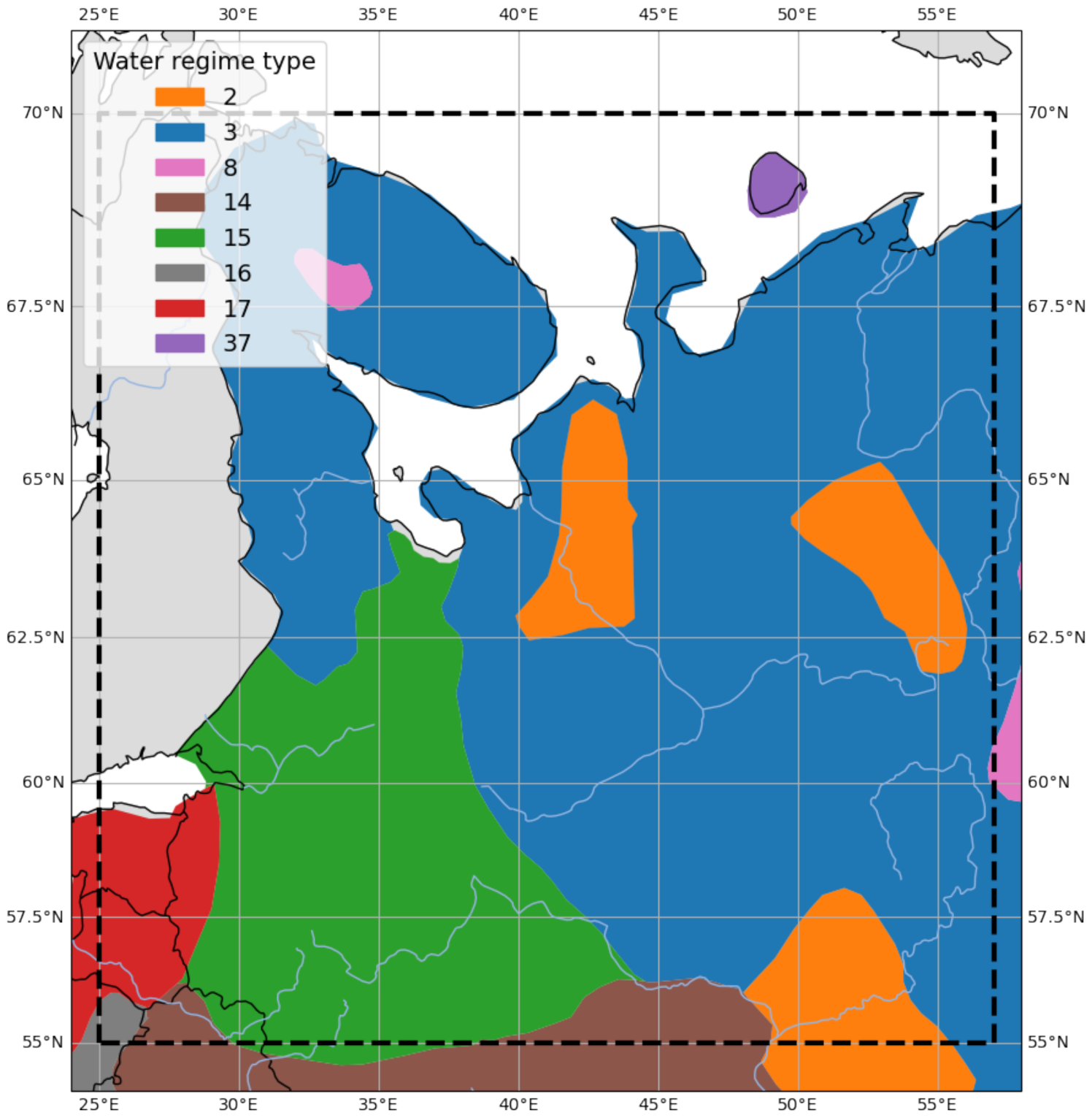
The map of the “Water regime of the rivers of Russia and neighboring territories” [26] has been cropped to fit the study region and digitized using standard tools provided in QGIS software [28]. Figure 1 shows the digitized map, and Table 1 describes water regime types depicted in Figure 1. In the presented study, we use the following definitions of the seasons of the year: winter (November–February), spring (March–May), and summer–autumn (June–October).
To move from qualitative to quantitative assessments, we propose the grid cell-based simplification of the digitized map–the conversion procedure under which every grid cell from the study region (with a spatial resolution of 0.5 × 0.5) is unambiguously attributed to a respective water type regime. The individual grid cell is assigned to the main major class based on the spatial majority for grid cells that intersect two or more polygons of different regime types.
2.3. Runoff Data
In the framework of the R5 project, extensive datasets of gridded runoff products have been developed for the studied region (for methodology, see [27,29]). These products include:
- Runoff reanalysis for the historical period (R5, 1979–2016);
- Future runoff projections (R5CH, 2006–2099) based on four GCMs (GFDL-ESM2M, HadGEM2-ES, IPSL-CM5A-LR, MIROC5) and three respective RCPs (RCP26, RCP60, RCP85) [30].
Runoff has been calculated using the GR4J hydrological model [31] and bias-corrected meteorological forcing data distributed in the framework of the ISIMIP project [32].
Typically, the studies on water regime types classification utilize station-based data. However, these data are not usually homogeneous in terms of spatial and temporal coverage. Thus, here we use gridded runoff reanalysis (R5) and runoff projection (R5CH) data to ensure spatiotemporal consistency. All products have a spatial resolution of 0.5 × 0.5 and daily temporal resolution. The data is freely available in open repositories [30].
2.4. Classification Approach
2.4.1. Random Forest Model
There are two general approaches for the classification of water regimes on distinct types: (1) empirical and (2) statistical [33]. The first approach uses expert rules to empirically derive the revised set of comprehensive types (classes). The second approach utilizes statistical procedures for automatic clustering (hierarchical or agglomerative) [33,34]. While the first approach is classic and in the roots of regional hydrology, it became too arbitrary and rigid to implement with an increasing amount of available data [33,35,36]. Thus, the modern studies on water regime classification are almost entirely based on the statistical models for clusterization. Instead, in the presented study, we want to combine two approaches—empirical and statistical. Here we let a machine learning model learn one of the available water regime classifications for the European part of Russia (Section 2.1) based on monthly runoff data (Section 2.3). In the case of an effective learning procedure, we will have a robust model that we could further implement for water regime type prediction using runoff projections as input (Section 2.3).
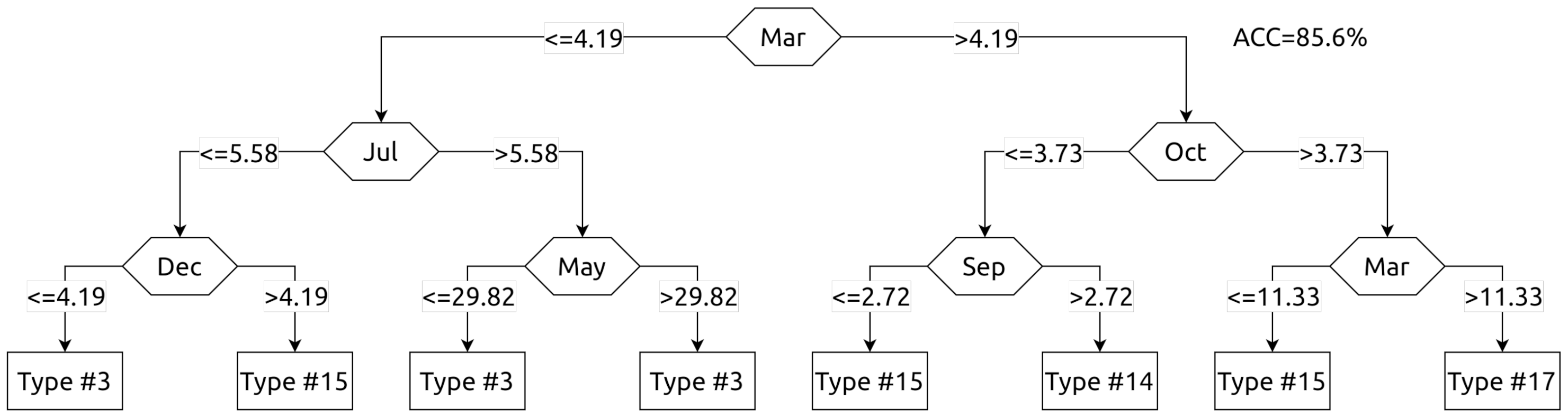
In the presented study, we use Random Forest [37] to derive the classification of water regimes on comprehensible types. The Random Forest model has been selected from the myriad of available classification algorithms because of its availability, prominence, and high efficiency in solving different research questions in water sciences, explicit interpretability of results, and proneness to overfitting [38,39]. Random Forest is an ensemble technique in its nature. It combines many independent nested models—Decision Trees (Figure 2)—where the results are averaged to provide a final estimate. Regarding classification tasks, each Decision Tree uses decision rules to split target variables into homogeneous classes based on predictor variables. In this way, an individual decision tree follows the general idea of empirical classification, i.e., deriving the set of expert rules that split available data into homogeneous classes. The difference is that an expert derives the set of hard-coded rules by experience, but Decision Tree–by the result of numerical optimization (learning). A detailed description of underlying computational algorithms of Random Forest is provided in [38,40].
2.4.2. Training Data Preprocessing
Following the general practice of water regime classification studies [24,33,34,35,36], we use climatological monthly runoff data. However, compared to classic approaches where descriptive statistics are derived from monthly data (e.g., means, deviations, ratios) to serve as input data for classification procedures, we rely only on monthly climatological means. The underlying assumption of that choice is that monthly data implicitly includes all the descriptive information, and the Random Forest model is advanced enough to extract these meaningful features. Thus, we prepare the training dataset as follows. First, for each grid cell, we extract the target variable—corresponding water regime type—based on the obtained grid cell-based map (Section 2.2). Second, for each grid cell, we extract daily runoff time series from R5 reanalysis for 1979–1991, which is representative and consistent with data used for water regimes map (Section 2.1) compilation. Then, that time series is aggregated from daily to monthly temporal resolution and recalculated as a percentage of the average annual flow. As a result, we have compiled a dataset that unambiguously determines input (12 values of relative monthly runoff) and output data (water regime type) for our Random Forest model.
2.4.3. Cross-Validation Procedure
The final classification model has been found by grid search procedure aiming to optimize the most sensitive Random Forest hyperparameter—the number of trees (10–100). For each hyperparameter value, the classification accuracy has been assessed using 5-fold stratified cross-validation. The model with the highest mean accuracy on the validation set has been selected for water regime types prediction. We used only open source and freely available software packages for computational workflow–NumPy [41], Pandas [42,43], GeoPandas [44], Xarray [45], and Scikit-learn [46].
2.5. Summary of the Proposed Workflow
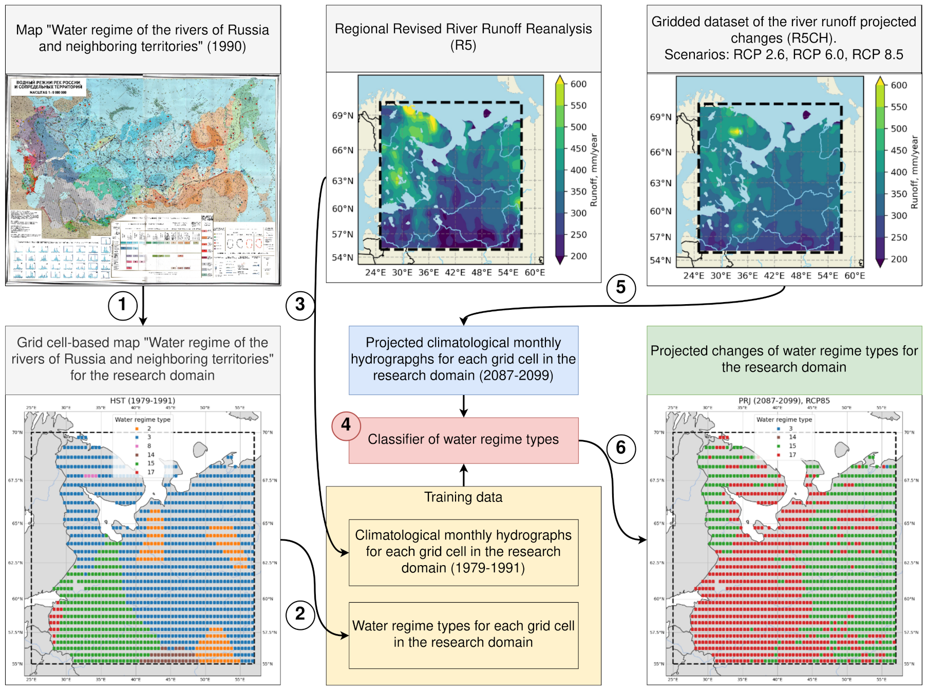
The schematic illustration of the proposed research workflow is shown in Figure 3.
The summary of the main steps depicted in Figure 3 is as follows:
- We digitize the map “Water regime of the rivers of Russia and neighboring territories” and simplify it in a grid cell-based manner (Section 2.1);
- For each grid cell, we extract the corresponding type of water regime;
- For each grid cell, we extract relative monthly runoff based on R5 historical runoff reanalysis for the period 1979–1991 (Section 2.3);
- Using the compiled dataset derived in steps 2 and 3, we train the Random Forest classification model using extensive grid search and cross-validation procedures (Section 2.4);
- For each grid cell, we extract the future projections of the relative monthly runoff based on the R5CH dataset that combines runoff estimates derived by using four GCMs and three RCPs for the period 2087–2099 (Section 2.3). The corresponding projected period (2087–2099) has been selected as the most distant from the historical reference period (1979–1991) with the same duration (13 years). We assume that due to that selection of periods, the obtained changes in the water regime types will be most pronounced; thus, better described and disseminated;
- Using the trained Random Forest model (Section 2.4) and a scenario of future projection of monthly runoff, we calculate the expected type of water regime at the end of the 21st century.
3. Results and Discussion
3.1. Determination of the Historical Baseline
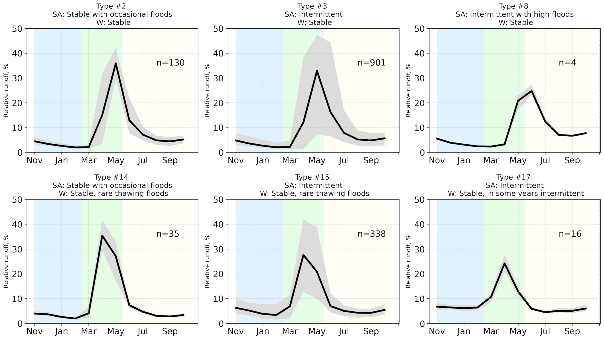
For each grid cell (n = 1424), climatological hydrographs and water regime type have been extracted for the reference period (1979–1991; historical, HST) from the R5 runoff reanalysis and the digitized map “Water regime of the rivers of Russia and neighboring territories”, respectively. Figure 4 illustrates the corresponding mean climatological hydrographs derived for each water regime type. It also shows the variability of individual cell’s climatological hydrographs for the respective water regime types. The number of grid cells of each water regime type and their relative coverage are shown in Table 2. Figure 5 highlights the distinct differences between different groups of water regime types we will analyze further.
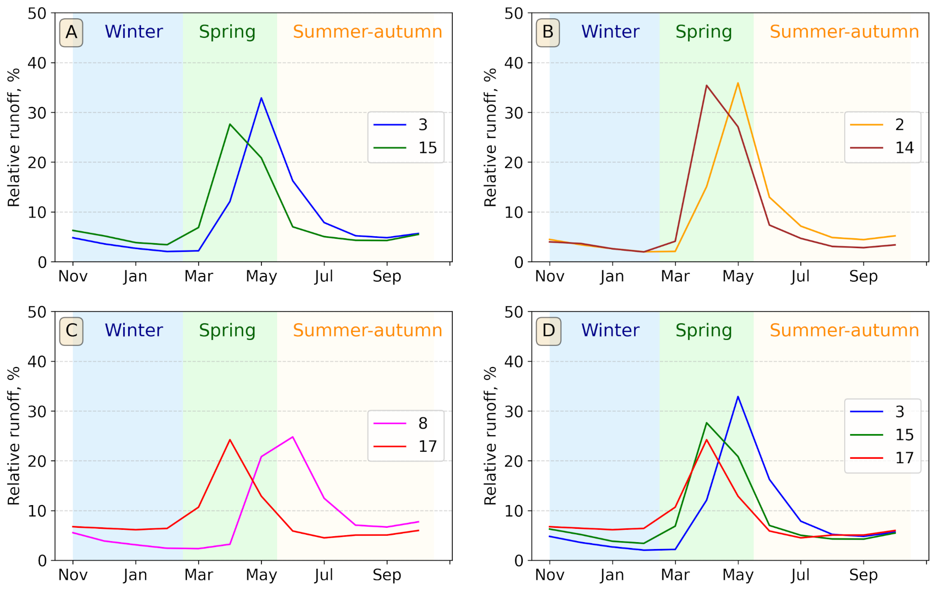
Climatological hydrographs and their variability (Figure 4 and Figure 5) clearly illustrate distinctive differences between presented water regime types. There are two major types of water regimes—3rd (SA: intermittent; W: stable. Hereafter, the abbreviations SA and W stand for summer–autumn and winter, respectively. See Table 1 for full descriptions.) and the 15th (SA: intermittent; W: stable, rare thawing floods). Both are characterized by the dominance of spring flood and intermittent summer low flow. The main difference between these two types is in the water regime of the winter period (Figure 5A). While for the 3rd type, low winter flow is stable, for the 15th type, the stable winter low flow could be interrupted by thawing floods [25]. Figure 5 also reveals the noticeable difference in spring flood properties. First, for the 3rd type, the runoff peak usually occurs in May, while April is for the 15th type. Second, the magnitude of the spring flood is also higher for the 3rd type rather than for the 15th. Third, the rising and falling limb for the 3rd type is symmetric, but it is skewed towards the longer falling limb for the 15th type. These differences could be attributed to the geographical location of the analyzed water regime types, where the 3rd type is located to the north of the 15th type.
The 2nd (SA: stable with occasional floods; W: stable) and 14th (SA: stable with occasional floods; W: stable, rare thawing floods) types of water regimes (Figure 5B) are closer to the 3rd (SA: intermittent; W: stable) and 15th (SA: intermittent; W: stable, rare thawing floods) types, respectively. Both are characterized by the dominance of spring flood and stable summer low flow with occasional floods, with the difference in winter low flow regimes similar to those for the 3rd and 15th types. Thus, the difference between these two groups of water regime types (2nd and 14th vs. 3rd and 15th) is in low summer flow: while for the 3rd and 15th types it is intermittent, for the 2nd and 14th types it is stable low water with occasional floods [25]. A higher magnitude of spring flood characterizes both 2nd and 14th types compared to 3rd and 15th types and the lower variance of nested climatological hydrographs that could result from the smaller presence of their areas (Table 2). The 2nd type is nested within the 3rd type, and the 14th type is adjacent to the 15th type.
The presence of minor water regime types—8th (SA: intermittent with high floods; W: stable) and 17th (SA: intermittent; W: stable, in some years intermittent)—is rare, with a total share of 1.4% (Figure 5C). The 17th type is closer to both 3rd (SA: intermittent; W: stable) and 15th (SA: intermittent; W: stable, rare thawing floods) types, with similar characteristics of summer low flow and dominance of spring flood, but with winter period characterized by stable low water, in some years intermittent [25]. Figure 5C shows that the 17th type of water regime could also be characterized by a lower magnitude of spring flood and higher low flow periods (both summer-autumn and winter periods). Regarding geographical location, the 17th type shares the SW-NE diagonal with the 3rd and 15th types and occupies the westernmost position (Figure 1 and Figure 5D). The 8th type of water regime is scarce with spring-summer flood and summer-autumn low flow periods with intermittent low water with floods, reaching the height of the maximum spring flood [25].
Despite its age of three decades, the water regime types classification provided by Evstigneev et al. [25] remains the most advanced and complete generalization of characteristics of the water regime of Russian rivers. The main feature of the considered classification (and it is also typical for the Soviet Union scientific school of hydrological sciences) is supervised, expert-centric regionalization of the analyzed territory on the finite number of distinct classes that can be visually and textually distinguished and represented on a map [24]. Moreover, the most up-to-date classification of water regime types of Russian rivers is available in the Russian National Atlas [47] and represents the generalized version of the presented map “Water regime of the rivers of Russia and neighboring territories,” developed by Evstigneev et al. [25], Evstigneev et al. [26]. The spatially connected and continuous representation of water regime types allows us to couple it with spatially and temporally consistent data of gridded runoff reanalysis. Thus, that coupling opens a way towards a consistent analysis of water regime types evolution both in space and in time.
3.2. Classification Model Accuracy
The classification model used for predictions of water regime types in the presented study has been derived using a pipeline of a grid search procedure and stratified 5-fold cross-validation (Section 2.4). The results show that the Random Forest model with 25 individual decision trees in an ensemble (parameter n_estimators = 25) showed the best prediction accuracy on test data of 91.6%. The obtained result is consistent with the result obtained in the study of Ivanov et al. [48], where the authors reached 90% accuracy utilizing a decision tree-based machine learning model (XGBoost) in water regime type identification for the 1945–1977 period. The Random Forest model has been re-calibrated on the entire dataset to derive the final model for water regime type predictions. The final Random Forest model is freely available [49] and could be used for water regime type prediction in the studied region (25–57 E; 55–70 N).
3.3. Projected Changes of Water Regime Types
Having the trained Random Forest model at hand, we calculated the expected type of water regime at the end of the 21st century (2087–2099) using different scenarios of future monthly runoff projections forced by four GCMs (GFDL-ESM2M, HadGEM2-ES, IPSL-CM5A-LR, MIROC5) and three RCPs (RCP26, RCP60, RCP85). For each RCP, the final predicted type of future water regime has been calculated using the hard majority rule voting based on the predicted types by four participating GCMs [50]. Furthermore, based on the analysis of individual predictions, we calculated the confidence level between different model scenarios. We consider high confidence if at least three models agree on the predicted type of water regime. In other cases, we consider the model confidence as low. In this way, calculating the model’s confidence is a simplified attempt to address prediction uncertainty.
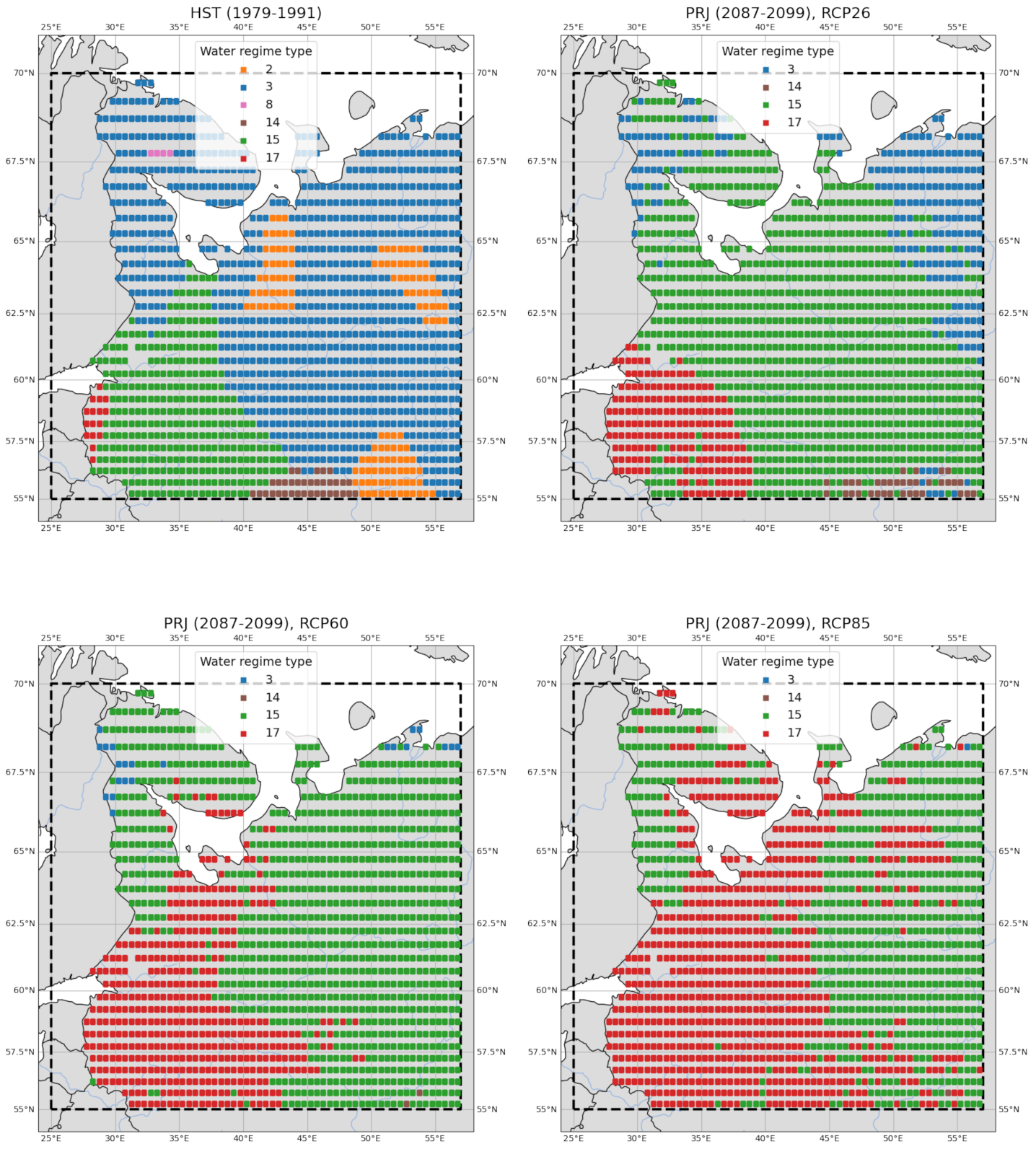
Figure 6 illustrates the spatial coverage and difference between historical (HST, 1979–1991) and projected (PRJ, 2087–2099) water regime types derived for different scenarios of greenhouse gas emissions (RCP26, RCP60, RCP85) at the end of the 21st century. The corresponding relative coverage of different water regime types in the study region is summarized in Table 3.
Compared to the historical period, where there were six types of water regimes, only four exist under the RCP26 scenario: 3rd (SA: intermittent; W: stable), 14th (SA: stable with occasional floods; W: stable, rare thawing floods), 15th (SA: intermittent; W: stable, rare thawing floods), and 17th (SA: intermittent; W: stable, in some years intermittent), while two entirely disappeared: the 2nd (SA: stable with occasional floods; W: stable) and 8th (SA: intermittent with high floods; W: stable). The disappeared types of water regimes—2nd and 8th—are related to those with stable phases of summer and winter flow and mountain rivers, respectively. Thus, under the RCP26 scenario, there is an expected change of water regime types towards decreasing low flow phases’ stability and a signal of the high vulnerability of mountain rivers under climate change [51,52].
The most pronounced increase in relative coverage is attributed to the 17th (SA: intermittent; W: stable, in some years intermittent; from 1.1 to 13.1%, 12 times more) and 15th (SA: intermittent; W: stable, rare thawing floods; from 23.7 to 69%, 2.9 times more) types. The coverage of the 3rd type (SA: intermittent; W: stable) dropped significantly from 63.3 to 15.4%. The 14th type (SA: stable with occasional floods; W: stable, rare thawing floods) of water regime saves relative coverage but shifts toward the east direction. Moreover, there is a clear water regime type pattern from southwest to northeast (Figure 6). While the pair of two major water regime types—3rd and 15th—remain the same between historical and projected (under RCP26 scenario) periods, with 87% and 84.4% of total coverage, the dominant type of water regime changed from 3rd on historical to 15th on projected period, respectively. In this way, obtained results confirm the primary direction of water regime change towards less stable summer and winter flows that can be interrupted by thaws, rain-induced floods, or droughts. From the visual comparison of the 3rd and 15th types of water regimes (Figure 5A), it is clear that while the spring flood will stay the dominant phase of the water regime, the flood peak will shift towards earlier occurrence and lower magnitude. In this way, the projected changes will touch all the major phases of the water regime: spring flood, and summer and winter low flow periods.
The revealed changes in projected water regime type spatial distribution under the RCP26 scenario at the end of the 21st century are consistent with the trends of water regime transformation in the 1945–2015 period, which are presented in Kireeva et al. [53], i.e., a decrease in the spring flood magnitude and volume, and an increase in low flows. Furthermore, Kireeva et al. [53] indicate that the current water regime of several rivers could hardly be attributed to the East European type of water regime according to Zaikov B.D.’s classification [54] due to significant changes in spring flood characteristics. Thus, identifying water regime types transition due to projected climate change remains a strong focus for providing up-to-date classifications of current and projected water regimes.
The analysis of the projected water regime changes under a more aggressive RCP60 scenario shows the intensification of the dominant transition processes. The number of presented water regimes is reduced to three (six for HST, four for RCP26). The 14th type (SA: stable with occasional floods; W: stable, rare thawing floods) almost disappeared, indicating a further decrease in the presence of water regime types characterized by stable summer low flow. The 15th (SA: intermittent; W: stable, rare thawing floods) and 17th (SA: intermittent; W: stable, in some years intermittent) types of water regimes make 90% of the total coverage. The 15th type remains dominant and saves its ratio compared to RCP26 but shifts to the northeast direction. The 17th type increased 2.5 times in comparison to RCP26 and continued its expansion to the northeast direction. The presence of the 3rd type is sporadic and is more associated with peripheral zones of the study area. Thus, the primary trend towards increasing the instability of low flow periods and earlier and lower spring floods is more pronounced for RCP60 than for RCP26.
The revealed changes are even more pronounced for the most aggressive scenario of climate change—RCP85. The number of presented water regime types decreased to only two (six for HST, four for RCP26, three for RCP60)—15th (SA: intermittent; W: stable, rare thawing floods) and 17th (SA: intermittent; W: stable, in some years intermittent). The disappeared 3rd type (SA: intermittent; W: stable) of the water regime also approves the change toward lower stability of low flow periods (Figure 5D). The 17th type becomes dominant under the RCP85 scenario with a stable increase from the historical period (1.1% for HST, 13.1% for RCP26, 31% for RCP60, 53.5% for RCP85). That also indicates the increasing instability of winter low flows characterized by increasing frequency of low flow interruption by mid-winter thaws. The spatial expansion of water regime types in the northeast direction remains persistent between all considered RCP scenarios.
3.4. Prediction Uncertainty
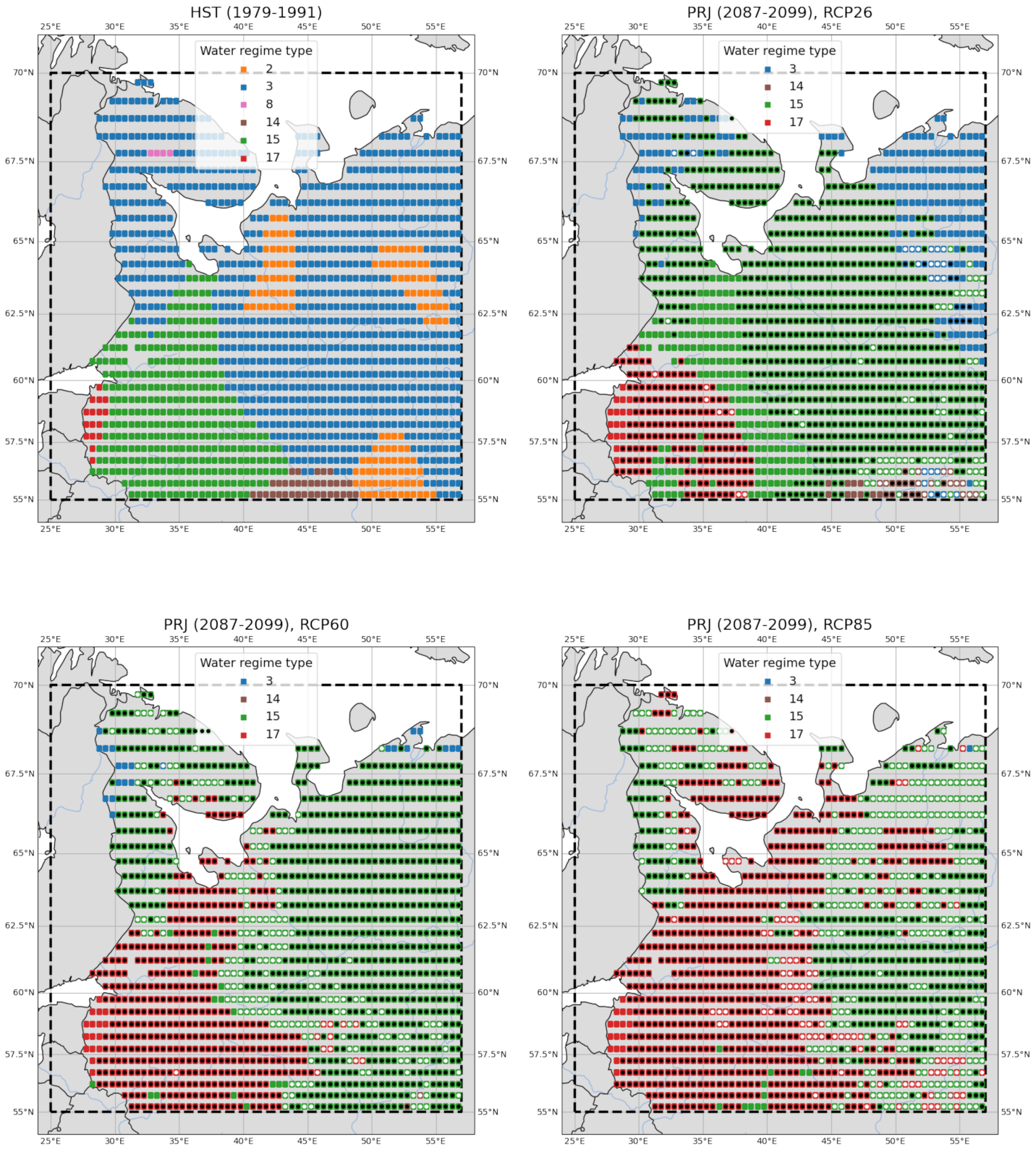
The presented study used a simple measure of uncertainty of water regime types prediction–the confidence between model predictions forced by different GCMs (Section 2). That confidence measure could take only two values: high (where at least three models agree on the predicted type of water regime) and low (in other cases). The spatial distribution of the predicted water regime types that is concerted with the confidence measure of these predictions is shown in Figure 7. The obtained results are also summarized in Table 4.
The obtained results present two most prominent messages: (1) the affected area of water regime changes increases with more aggressive RCP scenarios; (2) however, the model confidence decreases with more aggressive RCPs, yet the majority of predictions remains of high confidence. Thus, by the end of the 21st century, at least 73.6% of the study area will transit to different water regime types. The main directions of that transition–interruption of low flow periods by thaws, rain-induced floods or droughts, and earlier and lower spring floods—this agrees with the modern changes in runoff characteristics [24,53,55]. Thus, even following a less aggressive RCP scenario (RCP26), we could be confident in a substantial change of water regime in the northwest of Russia. Despite our confidence decreases with more aggressive RCP scenarios, the results still indicate a prominent signal of projected changes.
The obtained results (Figure 7) indicate that there are several reasons for low model confidence: (1) it is hard to distinguish between close types of water regime, e.g., 15th (SA: intermittent; W: stable, rare thawing floods) and 17th (SA: intermittent; W: stable, in some years intermittent; Figure 5D), (2) there are new, different types of water regime that are not represented during the training on a historical period, e.g., ones without strong spring flood, and (3) the disagreement between meteorological projections calculated by different GCMs increases with more aggressive RCPs [17,56] that leads to the disagreement in runoff estimates. The first issue could be observed as a boundary effect—when low confidence is attributed to areas close to boundaries between water regime types. It is the most prominent for predictions under the RCP60 scenario (Figure 7, boundary between 15th and 17th types in the middle). The remaining issues could randomly appear elsewhere, indicating the regions where more in-depth analysis is needed, e.g., the northeast and southeast parts of the study region and the Kola peninsula (Figure 7, RCP85 subplot).
4. Conclusions
In the presented study, we quantified the significant directions of water regime change in northwest Russia at the end of the 21st century compared to the historical period. It has been done by utilizing a wide range of research data and computational techniques. These are digitized maps of water regime types, regional runoff reanalysis and runoff projections data, and machine learning (Figure 3). By design, our study is focused on the detection of projected changes in water regime types rather than their attribution to driving mechanisms in the hydrological cycle. That is also reflected in the second research question, which begins with the interrogative word “How,” not “Why.” In this way, our study highlights and quantifies the “hot spots” of projected water regime change. That information could then be used as a starting point for the in-depth analysis of driving mechanisms behind the projected changes.
In the Introduction, we formulated two central research questions that we would like to investigate:
- Could a modern machine learning-based model classify water regime types based on climatological runoff hydrographs?
- If yes, how water regime types will change due to projected changes in global climate by the end of the 21st century?
Regarding the first research question, the obtained results of machine learning model training and evaluation (Section 3.2) confirmed the high efficiency of the Random Forest model in predicting the type of water regime based on climatological runoff hydrographs. The mean accuracy on independent test data reached 91.6%. We shared the trained Random Forest model in an open repository [49] to ensure research reproducibility.
Regarding the second research question, the obtained results (Figure 6, Table 3) reveal the two significant directions of water regime change projected by the end of the 21st century. The first direction is towards less stable summer and winter flows that can be frequently interrupted by thaws, rain-induced floods, or droughts. The second direction is towards the change of spring flood characteristics. While spring flood is expected to remain the dominant phase of the water regime, the flood peak will shift towards earlier occurrence and lower magnitude. Thus, we urge that the projected changes will touch all the major phases of the water regime in the study region: spring flood, and summer and winter low flow periods. Furthermore, we identified that the projected changes in water regime types are more pronounced in more aggressive RCP scenarios. The anticipated shift in water regime types will touch 73.6% of the study area under the RCP26 scenario and 99% under the most aggressive RCP85 scenario (Figure 7, Table 4).
The projected changes indicate the increasing instability of all major phases of the water regime in the study region. That also means more extreme events: thaws, rain-induced flash floods, droughts, or their combination. Altogether, that poses a significant challenge to local communities and water management authorities that have to find a robust strategy to adapt to the expected changes. As a scientific community, we also should pay more attention to the communication of our findings beyond research papers and reports–to reach regional communities and stakeholders.
Funding
The reported study was funded by the Russian Foundation for Basic Research (RFBR) according to the research project number 19-35-60005.
Data Availability Statement
The utilized runoff data (Section 2.3) and classification model (Section 2.4) are freely available in open repositories [30,49].
Acknowledgments
The author thanks Natalia Frolova (the Hydrology Department of the Lomonosov Moscow State University) for providing a guideline on scientific research in assessing changes in the water regime in Russia.
Conflicts of Interest
The author declares no conflict of interest.
References
- CRED. Natural Disasters 2019. 2020. Available online: https://emdat.be/sites/default/files/adsr_2019.pdf (accessed on 25 June 2020).
- United Nations Office for Disarmament Affairs. Human Cost of Disasters; United Nations: Herndon, VA, USA, 2020. [Google Scholar]
- UN World Water Development Report 2020. Available online: https://www.unwater.org/publications/world-water-development-report-2020/ (accessed on 25 June 2020).
- Blöschl, G.; Hall, J.; Viglione, A.; Perdigão, R.A.; Parajka, J.; Merz, B.; Lun, D.; Arheimer, B.; Aronica, G.T.; Bilibashi, A.; et al. Changing climate both increases and decreases European river floods. Nature 2019, 573, 108–111. [Google Scholar] [CrossRef] [PubMed]
- Blöschl, G.; Kiss, A.; Viglione, A.; Barriendos, M.; Böhm, O.; Brázdil, R.; Coeur, D.; Demarée, G.; Llasat, M.C.; Macdonald, N.; et al. Current European flood-rich period exceptional compared with past 500 years. Nature 2020, 583, 560–566. [Google Scholar] [CrossRef] [PubMed]
- WWAP (World Water Assessment Programme). The United Nations World Water Development Report 4: Managing Water under Uncertainty and Risk; UNESCO: Paris, France, 2012. [Google Scholar]
- WCRP Coupled Model Intercomparison Project (CMIP). Available online: https://www.wcrp-climate.org/wgcm-cmip (accessed on 25 June 2020).
- IPCC. Climate Change 1990: The Science of Climate Change; The Intergovernmental Panel on Climate Change: Geneva, Switzerland, 1996. [Google Scholar]
- IPCC. Global Warming of 1.5 °C: An IPCC Special Report on the Impacts of Global Warming of 1.5 °C above Pre-Industrial Levels and Related Global Greenhouse Gas Emission Pathways, in the Context of Strengthening the Global Response to the Threat of Climate Change, Sustainable Development, and Efforts to Eradicate Poverty; Intergovernmental Panel on Climate Change: Geneva, Switzerland, 2018. [Google Scholar]
- Maraun, D. Bias correction, quantile mapping, and downscaling: Revisiting the inflation issue. J. Clim. 2013, 26, 2137–2143. [Google Scholar] [CrossRef] [Green Version]
- Lange, S. Trend-preserving bias adjustment and statistical downscaling with ISIMIP3BASD (v1.0). Geosci. Model Dev. 2019, 12, 3055–3070. [Google Scholar] [CrossRef] [Green Version]
- Dankers, R.; Arnell, N.W.; Clark, D.B.; Falloon, P.D.; Fekete, B.M.; Gosling, S.N.; Heinke, J.; Kim, H.; Masaki, Y.; Satoh, Y.; et al. First look at changes in flood hazard in the Inter-Sectoral Impact Model Intercomparison Project ensemble. Proc. Natl. Acad. Sci. USA 2014, 111, 3257–3261. [Google Scholar] [CrossRef] [Green Version]
- Huang, S.; Kumar, R.; Flörke, M.; Yang, T.; Hundecha, Y.; Kraft, P.; Gao, C.; Gelfan, A.; Liersch, S.; Lobanova, A.; et al. Evaluation of an ensemble of regional hydrological models in 12 large-scale river basins worldwide. Clim. Chang. 2017, 141, 381–397. [Google Scholar] [CrossRef]
- Krysanova, V.; Donnelly, C.; Gelfan, A.; Gerten, D.; Arheimer, B.; Hattermann, F.; Kundzewicz, Z.W. How the performance of hydrological models relates to credibility of projections under climate change. Hydrol. Sci. J. 2018, 63, 696–720. [Google Scholar] [CrossRef]
- Olsson, J.; Arheimer, B.; Borris, M.; Donnelly, C.; Foster, K.; Nikulin, G.; Persson, M.; Perttu, A.M.; Uvo, C.B.; Viklander, M.; et al. Hydrological climate change impact assessment at small and large scales: Key messages from recent progress in Sweden. Climate 2016, 4, 39. [Google Scholar] [CrossRef]
- Gusev, E.; Nasonova, O.; Kovalev, E.; Ayzel, G. Modelling water balance components of river basins located in different regions of the globe. Water Resour. 2018, 45, 53–64. [Google Scholar] [CrossRef]
- Ayzel, G.; Izhitskiy, A. Climate change impact assessment on freshwater inflow into the Small Aral Sea. Water 2019, 11, 2377. [Google Scholar] [CrossRef] [Green Version]
- Rottler, E.; Bronstert, A.; Bürger, G.; Rakovec, O. Projected changes in Rhine River flood seasonality under global warming. Hydrol. Earth Syst. Sci. 2021, 25, 2353–2371. [Google Scholar] [CrossRef]
- Liu, W.; Yang, T.; Sun, F.; Wang, H.; Feng, Y.; Du, M. Observation-Constrained Projection of Global Flood Magnitudes With Anthropogenic Warming. Water Resour. Res. 2021, 57, e2020WR028830. [Google Scholar] [CrossRef]
- Giuntoli, I.; Prosdocimi, I.; Hannah, D.M. Going Beyond the Ensemble Mean: Assessment of Future Floods From Global Multi-Models. Water Resour. Res. 2021, 57, e2020WR027897. [Google Scholar] [CrossRef]
- von Brömssen, C.; Betnér, S.; Fölster, J.; Eklöf, K. A toolbox for visualizing trends in large-scale environmental data. Environ. Model. Softw. 2021, 136, 104949. [Google Scholar] [CrossRef]
- Gusev, E.; Nasonova, O.; Kovalev, E.; Ayzel, G. Possible climate change impact on river runoff in the different regions of the globe. Russ. Meteorol. Hydrol. 2018, 43, 397–403. [Google Scholar] [CrossRef]
- Schneider, C.; Laizé, C.L.R.; Acreman, M.C.; Flörke, M. How will climate change modify river flow regimes in Europe? Hydrol. Earth Syst. Sci. 2013, 17, 325–339. [Google Scholar] [CrossRef] [Green Version]
- Frolova, N.; Povalishnikova, E.; Kireeva, M. Classification and Zoning of Rivers by Their Water Regime: History, Methodology, and Perspectives. Water Resour. 2021, 48, 169–181. [Google Scholar] [CrossRef]
- Evstigneev, V.; Zaitsev, A.; Svatkova, T.; Chalov, R.; Shenberg, N. Water regime of the rivers of the USSR (high school map at a scale of 1: 8 000 000). Vestn. Mosk. Univ. Seriya 5 Geogr. 1990, 5, 10–16. [Google Scholar]
- Evstigneev, V.; Shenberg, N.; Anisimova, N.; Zaitsev, A. Water regime of the rivers of Russia and neighboring territories. In Map for Higher Education Institutions at Scale 1:8,000,000; Roskartografia: Moscow, Russia, 2001. [Google Scholar]
- Ayzel, G.; Kurochkina, L.; Zhuravlev, S. The influence of regional hydrometric data incorporation on the accuracy of gridded reconstruction of monthly runoff. Hydrol. Sci. J. 2020, 1–12. [Google Scholar] [CrossRef]
- QGIS Development Team. QGIS Geographic Information System; Open Source Geospatial Foundation: 2021. Available online: https://www.qgis.org (accessed on 30 September 2021).
- Ayzel, G.; Kurochkina, L.; Abramov, D.; Zhuravlev, S. Development of a Regional Gridded Runoff Dataset Using Long Short-Term Memory (LSTM) Networks. Hydrology 2021, 8, 6. [Google Scholar] [CrossRef]
- Ayzel, G.; Kurochkina, L.; Kazakov, E.; Krinitskiy, M.; Zhuravlev, S. Regional Revised River Runoff Reanalysis (R5): Historical and Projected River Runoff Data Set for the Northwest of the European Part of Russia. 2021. Available online: https://0-doi-org.brum.beds.ac.uk/10.5281/zenodo.4485391 (accessed on 30 September 2021).
- Perrin, C.; Michel, C.; Andréassian, V. Improvement of a parsimonious model for streamflow simulation. J. Hydrol. 2003, 279, 275–289. [Google Scholar] [CrossRef]
- Frieler, K.; Lange, S.; Piontek, F.; Reyer, C.P.O.; Schewe, J.; Warszawski, L.; Zhao, F.; Chini, L.; Denvil, S.; Emanuel, K.; et al. Assessing the impacts of 1.5° global warming–simulation protocol of the Inter-Sectoral Impact Model Intercomparison Project (ISIMIP2b). Geosci. Model Dev. 2017, 10, 4321–4345. [Google Scholar] [CrossRef] [Green Version]
- Haines, A.T.; Finlayson, B.L.; McMahon, T.A. A global classification of river regimes. Appl. Geogr. 1988, 8, 255–272. [Google Scholar] [CrossRef]
- Oueslati, O.; De Girolamo, A.M.; Abouabdillah, A.; Kjeldsen, T.R.; Lo Porto, A. Classifying the flow regimes of Mediterranean streams using multivariate analysis. Hydrol. Process. 2015, 29, 4666–4682. [Google Scholar] [CrossRef]
- Snelder, T.H.; Booker, D.J. Natural flow regime classifications are sensitive to definition procedures. River Res. Appl. 2013, 29, 822–838. [Google Scholar] [CrossRef]
- Berhanu, B.; Seleshi, Y.; Demisse, S.S.; Melesse, A.M. Flow regime classification and hydrological characterization: A case study of Ethiopian rivers. Water 2015, 7, 3149–3165. [Google Scholar] [CrossRef] [Green Version]
- Breiman, L. Random forests. Mach. Learn. 2001, 45, 5–32. [Google Scholar] [CrossRef] [Green Version]
- Tyralis, H.; Papacharalampous, G.; Langousis, A. A Brief Review of Random Forests for Water Scientists and Practitioners and Their Recent History in Water Resources. Water 2019, 11, 910. [Google Scholar] [CrossRef] [Green Version]
- Dramsch, J.S. Chapter One-70 years of machine learning in geoscience in review. In Advances in Geophysics; Moseley, B., Krischer, L., Eds.; Elsevier: Amsterdam, The Netherlands, 2020; Volume 61, pp. 1–55. [Google Scholar] [CrossRef]
- Loh, W.Y. Classification and regression trees. Wiley Interdiscip. Rev. Data Min. Knowl. Discov. 2011, 1, 14–23. [Google Scholar] [CrossRef]
- Harris, C.R.; Millman, K.J.; van der Walt, S.J.; Gommers, R.; Virtanen, P.; Cournapeau, D.; Wieser, E.; Taylor, J.; Berg, S.; Smith, N.J.; et al. Array programming with NumPy. Nature 2020, 585, 357–362. [Google Scholar] [CrossRef]
- McKinney, W. Data Structures for Statistical Computing in Python. In Proceedings of the 9th Python in Science Conference, Austin, TX, USA, 28 June–3 July 2010; pp. 56–61. [Google Scholar] [CrossRef] [Green Version]
- Pandas Development Team, T. Pandas-Dev/Pandas: Pandas. 2020. Available online: https://0-doi-org.brum.beds.ac.uk/10.5281/zenodo.3509134 (accessed on 30 September 2021).
- Jordahl, K.; den Bossche, J.V.; Fleischmann, M.; Wasserman, J.; McBride, J.; Gerard, J.; Tratner, J.; Perry, M.; Badaracco, A.G.; Farmer, C.; et al. Geopandas/Geopandas: V0.8.1. 2020. Available online: https://0-doi-org.brum.beds.ac.uk/10.5281/zenodo.3946761 (accessed on 30 September 2021).
- Hoyer, S.; Hamman, J. xarray: N-D labeled arrays and datasets in Python. J. Open Res. Softw. 2017, 5. [Google Scholar] [CrossRef] [Green Version]
- Pedregosa, F.; Varoquaux, G.; Gramfort, A.; Michel, V.; Thirion, B.; Grisel, O.; Blondel, M.; Prettenhofer, P.; Weiss, R.; Dubourg, V.; et al. Scikit-learn: Machine Learning in Python. J. Mach. Learn. Res. 2011, 12, 2825–2830. [Google Scholar]
- The Russian National Atlas. Available online: xn–80aaaa1bhnclcci1cl5c4ep.xn–p1ai/cd2/190/190.htm (accessed on 25 June 2020).
- Ivanov, A.; Samsonov, T.; Frolova, N.; Kireeva, M.; Povalishnikova, E. Objective classification of changes in water regime types of the Russian Plain rivers utilizing machine learning approaches. In Proceedings of the EGU General Assembly Conference Abstracts, Vienna, Austria, 4–8 May 2020; p. 11553. [Google Scholar]
- Ayzel, G. Random Forest-Based Model for Water Regime Type Prediction in the Northwest of the European Part of Russia. 2021. Available online: https://0-doi-org.brum.beds.ac.uk/10.5281/zenodo.4966175 (accessed on 30 September 2021).
- Sheng, V.S.; Zhang, J.; Gu, B.; Wu, X. Majority Voting and Pairing with Multiple Noisy Labeling. IEEE Trans. Knowl. Data Eng. 2019, 31, 1355–1368. [Google Scholar] [CrossRef]
- Rets, E.P.; Durmanov, I.N.; Kireeva, M.B.; Smirnov, A.M.; Popovnin, V.V. Past ‘peak water’ in the North Caucasus: Deglaciation drives a reduction in glacial runoff impacting summer river runoff and peak discharges. Clim. Chang. 2020, 163, 2135–2151. [Google Scholar] [CrossRef]
- Zemp, M.; Frey, H.; Gärtner-Roer, I.; Nussbaumer, S.U.; Hoelzle, M.; Paul, F.; Haeberli, W.; Denzinger, F.; Ahlstrøm, A.P.; Anderson, B.; et al. Historically unprecedented global glacier decline in the early 21st century. J. Glaciol. 2015, 61, 745–762. [Google Scholar] [CrossRef] [Green Version]
- Kireeva, M.; Frolova, N.; Rets, E.; Samsonov, T.; Entin, A.; Kharlamov, M.; Telegina, E.; Povalishnikova, E. Evaluating climate and water regime transformation in the European part of Russia using observation and reanalysis data for the 1945–2015 period. Int. J. River Basin Manag. 2020, 18, 491–502. [Google Scholar] [CrossRef]
- Zaikov, B. Average runoff and its distribution per year on the territory of the USSR. Proc. Natl. Res. Univ. Main Dep. Hydrometeorol. Serv. USSR IV 1946, 24, 67–95. [Google Scholar]
- Kireeva, M.B.; Rets, E.P.; Frolova, N.L.; Samsonov, T.E.; Povalishnikova, E.S.; Entin, A.L.; Durmanov, I.N.; Ivanov, A.M. Occasional Floods on the Rivers of Russian plain in the 20th–21st centuries. Geogr. Environ. Sustain. 2020, 13, 84–95. [Google Scholar] [CrossRef]
- Nasonova, O.N.; Gusev, Y.M.; Kovalev, E.E.; Ayzel, G.V. Climate change impact on streamflow in large-scale river basins: Projections and their uncertainties sourced from GCMs and RCP scenarios. Proc. Int. Assoc. Hydrol. Sci. 2018, 379, 139–144. [Google Scholar] [CrossRef]
Figure 1.
Digitized map of water regime types. A detailed description of the legend is provided in Table 1.
Figure 1.
Digitized map of water regime types. A detailed description of the legend is provided in Table 1.

Figure 2.
A single decision tree. The numbers on the arrows indicate the relative monthly river runoff.
Figure 2.
A single decision tree. The numbers on the arrows indicate the relative monthly river runoff.

Figure 3.
Illustration of the proposed computational workflow. Numbers in circles represent consecutive computational steps.
Figure 3.
Illustration of the proposed computational workflow. Numbers in circles represent consecutive computational steps.

Figure 4.
Monthly climatological hydrographs for different types of water regimes. Background color represents different seasons: blue for winter (November–February), green for spring (March–May), and yellow for summer–autumn (June–October). The abbreviations SA and W in the title refer to summer–autumn and winter periods, respectively.

Figure 5.
Pairwise comparison of monthly climatological hydrographs for different types of water regime. (A): the 3rd (SA: intermittent; W: stable) and 15th (SA: intermittent; W: stable, rare thawing floods); (B): the 2nd (SA: stable with occasional floods; W: stable) and 14th (SA: stable with occasional floods; W: stable, rare thawing floods); (C): the 8th (SA: intermittent with high floods; W: stable) and 17th (SA: intermittent; W: stable, in some years intermittent); (D): the 3rd (SA: intermittent; W: stable), 15th (SA: intermittent; W: stable, rare thawing floods), and 17th (SA: intermittent; W: stable, in some years intermittent).

Figure 6.
Historical (HST; 1979–1991) and projected (PRJ; 2087–2099) water regime types under different RCPs (RCP26, RCP60, RCP85).
Figure 6.
Historical (HST; 1979–1991) and projected (PRJ; 2087–2099) water regime types under different RCPs (RCP26, RCP60, RCP85).

Figure 7.
Historical (HST; 1979–1991) and projected (PRJ; 2087–2099) water regime types under different RCPs (RCP26, RCP60, RCP85). Black and white marks highlight high and low model confidence, respectively.
Figure 7.
Historical (HST; 1979–1991) and projected (PRJ; 2087–2099) water regime types under different RCPs (RCP26, RCP60, RCP85). Black and white marks highlight high and low model confidence, respectively.


Table 1.
The definition of derived water regime types for the territory of northwest Russia (based on Evstigneev et al. [25], Evstigneev et al. [26]).
| Water Regime Type Number | High-Water Phase | Summer-Autumn | Winter |
|---|---|---|---|
| 2 | Spring flood | Stable low water with occasional floods | Stable low water |
| 3 | Spring flood | Intermittent low water | Stable low water |
| 8 | Spring-summer flood | Intermittent low water with floods, reaching the height of the maximum spring flood | Stable low water |
| 14 | Spring flood | Stable low water with occasional floods | Stable low water, in rare winters interrupted by thawing floods |
| 15 | Spring flood | Intermittent low water | Stable low water, in rare winters interrupted by thawing floods |
| 16 | Spring flood | Stable low water with occasional floods | Stable low water, in some years intermittent |
| 17 | Spring flood | Intermittent low water | Stable low water, in some years intermittent |
| 37 | Temporary waterways of the Arctic islands | ||
Table 2.
Characteristics of the spatial distribution of the presented water regime types.
| Water Regime Type Number | Number of Grid Cells | Relative Coverage, % |
|---|---|---|
| 2 | 130 | 9.1 |
| 3 | 901 | 63.3 |
| 8 | 4 | 0.3 |
| 14 | 35 | 2.5 |
| 15 | 338 | 23.7 |
| 17 | 16 | 1.1 |
Table 3.
The percentage of the total study area under each water regime type derived for the historical and projected periods.
Table 3.
The percentage of the total study area under each water regime type derived for the historical and projected periods.
| Water Regime Type Number | HST | PRJ, RCP 2.6 | PRJ, RCP 6.0 | PRJ, RCP 8.5 |
|---|---|---|---|---|
| 2 | 9.1 | 0 | 0 | 0 |
| 3 | 63.3 | 15.4 | 1.5 | 0.1 |
| 8 | 0.3 | 0 | 0 | 0 |
| 14 | 2.5 | 2.5 | 0.1 | 0.1 |
| 15 | 23.7 | 69 | 67.4 | 46.3 |
| 17 | 1.1 | 13.1 | 31 | 53.5 |
Table 4.
Relative affected area and classifiers’ confidence.
| Scenario | Relative Affected Area, % | Low Confidence, % | High Confidence, % |
|---|---|---|---|
| RCP 2.6 | 73.6 | 10 | 90 |
| RCP 6.0 | 96.2 | 15 | 85 |
| RCP 8.5 | 98 | 28 | 72 |
Publisher’s Note: MDPI stays neutral with regard to jurisdictional claims in published maps and institutional affiliations. |
© 2021 by the author. Licensee MDPI, Basel, Switzerland. This article is an open access article distributed under the terms and conditions of the Creative Commons Attribution (CC BY) license (https://creativecommons.org/licenses/by/4.0/).
Share and Cite
MDPI and ACS Style
Ayzel, G. Machine Learning Reveals a Significant Shift in Water Regime Types Due to Projected Climate Change. ISPRS Int. J. Geo-Inf. 2021, 10, 660. https://0-doi-org.brum.beds.ac.uk/10.3390/ijgi10100660
AMA Style
Ayzel G. Machine Learning Reveals a Significant Shift in Water Regime Types Due to Projected Climate Change. ISPRS International Journal of Geo-Information. 2021; 10(10):660. https://0-doi-org.brum.beds.ac.uk/10.3390/ijgi10100660
Chicago/Turabian StyleAyzel, Georgy. 2021. "Machine Learning Reveals a Significant Shift in Water Regime Types Due to Projected Climate Change" ISPRS International Journal of Geo-Information 10, no. 10: 660. https://0-doi-org.brum.beds.ac.uk/10.3390/ijgi10100660
Note that from the first issue of 2016, this journal uses article numbers instead of page numbers. See further details here.