High Influencing Pattern Discovery over Time Series Data

Abstract

A spatial co-location pattern denotes a subset of spatial features whose instances frequently appear nearby. High influence co-location pattern mining is used to find co-location patterns with high influence in specific aspects. Studies of such pattern mining usually rely on spatial distance for measuring nearness between instances, a method that cannot be applied to an influence propagation process concluded from epidemic dispersal scenarios. To discover meaningful patterns by using fruitful results in this field, we extend existing approaches and propose a mining framework. We first defined a new concept of proximity to depict semantic nearness between instances of distinct features, thus applying a star-shaped materialized model to mine influencing patterns. Then, we designed attribute descriptors to perceive attributes of instances and edges from time series data, and we calculated the attribute weights via an analytic hierarchy process, thereby computing the influence between instances and the influence of features in influencing patterns. Next, we constructed influencing metrics and set a threshold to discover high influencing patterns. Since the metrics do not satisfy the downward closure property, we propose two improved algorithms to boost efficiency. Extensive experiments conducted on real and synthetic datasets verified the effectiveness, efficiency, and scalability of our method.

1. Introduction

In the past two decades, spatial co-location pattern mining has been a hot topic in the field of spatial data mining. After Shekhar et al. [1] first introduced the notion of spatial co-location patterns in 2001, many experts and scholars devoted themselves to this field and achieved abundant results. Thus far, the mining of spatial co-location patterns and extended patterns has been widely applied in public governance and traffic management and services, among others [2,3,4].

Currently, the COVID-19 pandemic has become a major worldwide event that seriously endangers human health and public safety. It has profoundly impacted all aspects of the world, and it has attracted increasing attention and in-depth study. Most existing research on the spread of epidemics focuses on practical applications, e.g., predictions of scale or effects of control measures, and little focuses on the pattern recognition in epidemic dispersal scenarios. Since the mechanisms of public opinion transmission and epidemic dispersal are similar [5,6,7], with the former being a hot topic of online community influence analysis, it is possible to view an epidemic as an influence between cities and to conclude an influence propagation process from epidemic dispersal scenarios. Therefore, the authors of this study intend to take advantage of the findings of spatial co-location pattern mining fields and explore meaningful high influencing patterns in an influence propagation process.

A typical paradigm for co-location pattern mining research can be described as follows: Given a set of spatial features F = $\left\{f_1,f_2, \dots , f_m\right\}$ and a set of instances O = $\left\{o_1,o_2, \dots , o_n\right\}$, each instance $o_i$ $\in$ O corresponding to a feature $f_i$ $\in$ F denotes an object at a specified location. A spatial co-location pattern is defined as a subset c = $\left\{f_1,f_2, \dots , f_k\right\}$ of spatial feature set F, whose instances are co-located together in the geographic space. Generally, two instances are adjacent if their spatial distance is not larger than a preset distance threshold R. When a set of instances I = $\left\{i_1,i_2, \dots , i_k\right\}$ satisfies the state that an arbitrary pair of instances in I are adjacent, I covers all features in c, and any subset of I cannot cover all features in c, the set I is reckoned as a row instance of c, denoted by row_instance(c). All row instances form a table instance of c, denoted by table_instance(c). The participation ratio of feature $f_i$ in c (denoted as PR(c, $f_i$)) is calculated by $\left|{\pi }_{f_i}Table\_instance\left(c\right)\right|/\left|Table\_instance\left(\left\{f_i\right\}\right)\right|$, which is the number of non-repetitive instances of feature $f_i$ involved in table_instance(c) divided by total instances of $f_i$. Participation index PI(c) of c takes the minimum PR(c$,f_i$) in c. Pattern c is prevalent if PI(c) is no less than a given threshold PI_threshold. Similarly, we first defined a new proximate relation for instances of distinct features, then found the influencing patterns based on the proximate relations, and next designed a measurement and set a threshold to identify the high influencing patterns whose measurements meet the threshold.

Construct new proximate relations: In order to construct new proximate relations between instances of distinct features, we reviewed the theoretical basis by which traditional spatial co-location pattern mining adopts spatial proximity, i.e., the first law of geography (or called Tobler’s first law (TFL)), alleging that everything is related to everything else but near things are more related to each other [8,9]. Based on this law, traditional spatial co-location pattern mining uses spatial distance or combined distance [10] to measure spatial nearness. In epidemic dispersal scenarios, viruses spread with infectors among streams of people, so neighbor cities in a space may have no or little association when there are no or few personnel exchanges; meanwhile, a strong association may exist between two cities that are far away but have frequent exchanges on a large scale, and in these contexts, spatial distance is no longer the dominant factor for reflecting the sematic proximate relations between instances on influence. A literature search revealed that, in a study on SARS dispersal in 2003, Li et al. [11] found that the semantic proximity between cities is closely related to the flows of people, and Brockmann et al. [12] noticed that human travel is responsible for the geographical spread of human infectious diseases. Therefore, it is feasible to construct new semantic proximate relations between instances of distinct features (i.e., cities of distinct categories) based on the flow of infectors and identify high influencing patterns accordingly.

In general, a neighborhood relation must satisfy the conditions of reflexivity, symmetry, and being non-negative bounded. That is the case for spatial proximity. However, in the case of influence propagation processes abstracted from epidemic dispersal scenarios, flows show the directions of influential media (i.e., infectors) with influence (i.e., viruses of epidemics). To solve the problem, we separated the fact of exchanges of influential media from their directions; that is, we decided to regard exchanges of influential media between instances of distinct features as the premise for judging semantic proximity between instances, and the directions of flows was considered in the influence calculation.

Influence calculation: Previous studies have usually mined spatial co-location patterns and extended patterns by means of external characteristics such as spatial distance, instance distribution, or statistics, so it has been difficult for them to deal with situations where complex interactions between organisms lead to their own changes. For instance, Barua et al. [13] used statistical methods to study the nesting behaviors of two kinds of ants and explore their biological dependence. They did not find definite evidence of spatial correlation between the two neighboring organisms, but the existing co-location pattern mining approaches can reveal an illusory correlation between them. In view of this, Duan et al. [14] proposed a method for mining co-location patterns without autocorrelation between species. Therefore, the authors of this study introduced influence-related time series attribute data of instances to describe the cumulative influence between instances of distinct features at different moments of an influence propagation process.

We first defined a semantic proximity relationship, i.e., two instances of distinct features are proximate if they exchange influential media. To simplify the analysis, the relationship is assigned a Boolean value of 0 (not proximate) or 1 (proximate). The relationship satisfies the properties of non-negative bounds, symmetry, and reflexivity (please refer to the proof B1 in Appendix B), and it can be used to describe semantic proximity between instances. Accordingly, with reference to the existing sub-prevalent co-location pattern [15,16], we propose a new kind of influencing patterns (IPs for short), where each feature of the pattern has at least one instance proximate to the instances of the other features of the pattern. Next, we set the flowing directions of influential media as the influencing directions between instances of distinct features, computed the influence between instances and then the influence of features in IPs with the preprocessed data of multi-dimensional attribute vectors perceived over time series data, attributed weights obtained from pairwise comparisons to obtain star influence ratio (SIR) values for features in IPs, and finally defined a metric of the star influence index (SII) by taking the minimum star influence ratio to measure the influencing levels of IPs and assign an SII_threshold to filter high IPs.

In summary, the contributions of this study include:

• For an influence propagation process abstracted from epidemic dispersal scenarios, we define a semantic proximate relationship to describe the nearness between instances of distinct features and accordingly propose a novel influencing pattern, and we further introduce a high influencing pattern based on the directions of influence and inner changes in instances perceived by an attribute-aware analysis of time series data to meet the needs for pattern discovery in the influence propagation process.
• We propose a framework for mining high IPs, design a Benchmark algorithm wherein we apply a top–down method to identify IPs to implement it, utilize a three-layer hashmap structure to store the IPs, compute the influence between instances and the influence of features in the IPs by using preprocessed multi-dimensional attribute vectors and attribute weights, and design influencing metrics to filter high IPs. As the metrics do not satisfy the downward closure property, we analyze two time-saving properties, propose two corresponding pruning strategies, and thus design two improved algorithms to boost efficiency.
• Extensive experiments were conducted on real and synthetic datasets, and the experimental results verified the effectiveness, efficiency, and scalability of our methods.

The rest of this study is organized as follows. Section 2 introduces related works. Section 3 provides definitions and the problem statement. Section 4 describes our mining framework, three algorithms, and time complexity analysis. Section 5 depicts the data and their preprocessing; it also presents our experiments on the effectiveness, efficiency, and scalability of the algorithms. Finally, Section 6 summarizes the study and discusses future research directions. Additionally, Appendix A lists the notation of the proposed algorithms in

Table A1. Notation used in proposed Listing 1, Listing 3 and Listing 4 and called functions (in alphabetic order).

Notation	Description
Cs	A set of all candidate patterns
HIPs	A set of all high influencing patterns
HIPsk-1	A set of all size-k-1 high influencing patterns
${\mathrm{IFIP}}_{c,f_i }$	Influence of feature fi in pattern c
IPs	A set of all influencing patterns
IPsk	A set of all size-k influencing patterns
Ns	A set of all star neighbor instance sets
${\mathrm{SII}}_c$	Star influence index of pattern c
${\mathrm{SIR}}_{c,{ f}_i}$	Star influence ratio of feature fi in pattern c
${\mathrm{SPI}}_c$	An upper bound index for star influence index of pattern c
${\mathrm{SPI}}_{{\mathrm{ns}}_{c,f_i}}$	Star participation instances of feature fi in pattern c
${\mathrm{SRI}}_{c,{ f}_i}$	Star row instances of feature fi in pattern c

, and Appendix B provides proofs of the semantic proximity relationship properties, Lemma 1 and Lemma 2.

2. Related Works

The authors of this study aimed to discover high IPs from an influence propagation process as reflected by epidemic dispersal scenarios. Our work extended the use of spatial co-location pattern mining based on the absorption of research findings in the fields of influence analysis and spatio-temporal pattern mining. We elaborate the related works in three aspects as follows.

2.1. Spatial Co-Location Pattern Mining

Shekhar et al. [1] first introduced the concept of spatial co-location patterns and proposed an event-centric approach adopting Apriori generation in 2001, and then Huang et al. [17] developed a full-join algorithm with a minimal participation ratio for discovering prevalent co-location patterns in 2004. As the statistically meaningful measurement of patterns has become more reasonable, many subsequent studies continue to use it, but mass join operations require extensive time. Thus, Yoo et al. [18,19] proposed a partial-join approach to divide instances into disjoint clusters and a join-less method based on a star neighbor materialized model to avoid join operations. Wang et al. [20,21] proposed new join-less approaches, i.e., CPI-tree- and iCPI-tree-based algorithms to speed up calculations of table instances, and they proved that their tree structures were effective for fast co-location mining. Yao et al. [22] reckoned prevalent size-2 co-locations as sparse undirected edges, and they adopted a degeneracy-based maximal clique mining method to generate candidate maximal co-locations and introduced a hierarchical verification approach to build a condensed instance tree for storing instance cliques, thus saving costs in computation and storage. Bao et al. [23] proposed an instance-driven schema and a neighborhood-driven schema to generate cliques and transformed them into a two-layer hash structure by which the prevalence of co-location patterns can be efficiently calculated without the identification of the row-instances of co-location patterns. Following studies on efficiency boosting, this field grew into a flourishing family with abundant fruitful results, including maximal clique and maximal prevalent co-location mining [24], high utility co-location mining [25], and fuzzy analysis [26]. Chen [27] first proposed a new concept of impact from buffers of extended spatial objects and designed a high impact measure to replace a participation ratio measure for co-location mining. This system can be used to compare the impacts that supermarkets and groceries exert on consumers. Fang et al. [28] introduced multi-dimensional attributes for spatial instances and applied information entropy technology to construct an influence measure based on the amount of neighbors and the similarity of neighbor pairs’ attributes, thus allowing for the discovery of high influence co-locations from instances with attributes. Lei et al. [29] used the cosine function to simulate the property of diminishing influence with distance, and they proposed high influence co-locations in which multiple pollution sources affected cancer patients. As cliques are too strict to reflect real world scenes, Ma et al. [30] observed that central instances usually had more neighbors than non-central instances in a star-shaped materialized model, so they proposed a new approach to mine sub-prevalent co-locations with dominant features. Although many notions and methods have been proposed for co-location mining, they are not applicable to an influence propagation process where space is anisotropic.

2.2. Influence Analysis

Influence analysis is another hot spot that has aroused researchers’ enthusiasm for in-depth study and wide applications, including influence evaluation on nodes [31], attribute-based treatment [32], community partition [33], and influence propagation [34]. Shang et al. [31] used an analytic hierarchy process method for constructing judgment matrices with multi-dimensional attributes, evaluated attribute weights, and calculated weights on nodes and edges to form a weighted topological network; they subsequently computed the influence of nodes with Weibo reposting and non-reposting probabilities. Li et al. [32] built a hierarchical tree based on the attributes associated with locations and dispersed the locations into different segments by using the Voronoi partition method, and then they used the four-color mapping theorem for coloring polygons to quickly choose virtual locations and protect privacy. Citraro et al. [33] introduced a bottom-up low complexity approach (EVA) to identify network-hidden mesoscale topologies by optimizing structural and attribute-homophilic clustering criteria. Subbian et al. [34] realized that information flow trends and influencers in social networks have become increasingly relevant, so they proposed an algorithm to mine the information flow patterns and then leverage an approach to determine key influencers in networks. Although research on influence analysis has achieved fruitful insights that can be considered for reference, few have considered the spatial characteristics of objects or the influence between instances of distinct categories. Moreover, research in the fields of influence analysis and co-location mining has seldom been fused.

2.3. Spatio-Temporal Pattern Discovery

In the era of big data, the scale and growth of data have expanded tremendously. Therefore, spatio-temporal pattern mining has grown to be an important research field. Yoo et al. [35] introduced a temporal dimension and identified co-evolving spatial event sets by applying an existing spatial co-location pattern mining approach on each timestamp. To cut down expensive costs of prevalence calculation, Celik et al. [36] proposed a method for mining mixed drive spatio-temporal co-location patterns and designed combined indices that satisfied anti-monotone conditions to prune the search space. They also mined persistently occurring and top-K ordering spatio-temporal co-location patterns [37,38]. Qian et al. [39] studied the spread patterns of spatio-temporal co-occurrences over zones. Celik et al. [40] proposed a new method for mining partial spatio-temporal co-occurrence patterns by first discovering spatially prevalent co-occurrence patterns then calculating temporal prevalence indices to filter those prevalent patterns. To consider the linkages between time slots, Qian et al. [41] introduced the influence of a time interval between features into the interest measure and proposed a sliding window model with weights to mine spatio-temporal co-location patterns. Huang et al. [42] proposed sequence pattern and corresponding mining approaches for a scenario of an epidemic disease spreading among different features.

In addition, this study concerns the latest progress in related interdisciplinary fields, e.g., mechanisms of epidemic dispersal [43], dynamic pattern mining of spatio-temporal data [44,45,46,47], and attribute-aware analysis [48]. Within this context, Hufnagel et al. [43] introduced a probabilistic model that described the worldwide spread of infectious diseases and achieved good agreement with published case reports, which showed that the high degree of predictability was caused by the strong heterogeneity of their network. Chen et al. [44] mined recurring co-movement patterns from trajectories of objects in a consecutive period of time. Hu et al. [45] proposed dynamic co-location mining in view of the fact that the definition of the participation ratio for a traditional co-location cannot reflect two or more feature changes in the same proportion and omits some meaningful patterns. Moosavi et al. [46] introduced a geo-spatiotemporal pattern discovery framework that defined a semantic neighborhood and proposed a propagation pattern to reveal common cascading forms of geospatial objects in a region, and they proposed another influential pattern to demonstrate the impact of long-term geospatial objects on their neighborhood. Shekhar et al. [47] reviewed recent computational techniques and tools in spatio-temporal data mining and asserted that the vast majority of present research was still in Euclidean space, but the unique asymmetric neighborhood and directionality of the neighborhood relationship, e.g., anisotropy and flow direction, required by the spatio-temporal network structure call for novel spatio-temporal statistical foundations and new computational approaches for spatio-temporal network data mining. Feng et al. [48] aimed to find a region elsewhere with area and multiple attributes most similar to a specified region.

From the perspective of the aforementioned research, it can be seen that the simplistic definition of existing spatio-temporal neighborhoods, i.e., spatial nearness based on a Euclidean or Cartesian system and temporal overlap, has hindered traditional explorations of the influence of leapfrog transmission, which reflects an anisotropic space. Therefore, based on latest research, the authors of this study defined a new proximity relationship based on influential flows that perceived attributes of instances and edges from spatio-temporal data, thus allowing us to mine high IPs within a specified period for the studied scenarios.

3. Definitions and Problem Statement

3.1. Definitions and Formulae

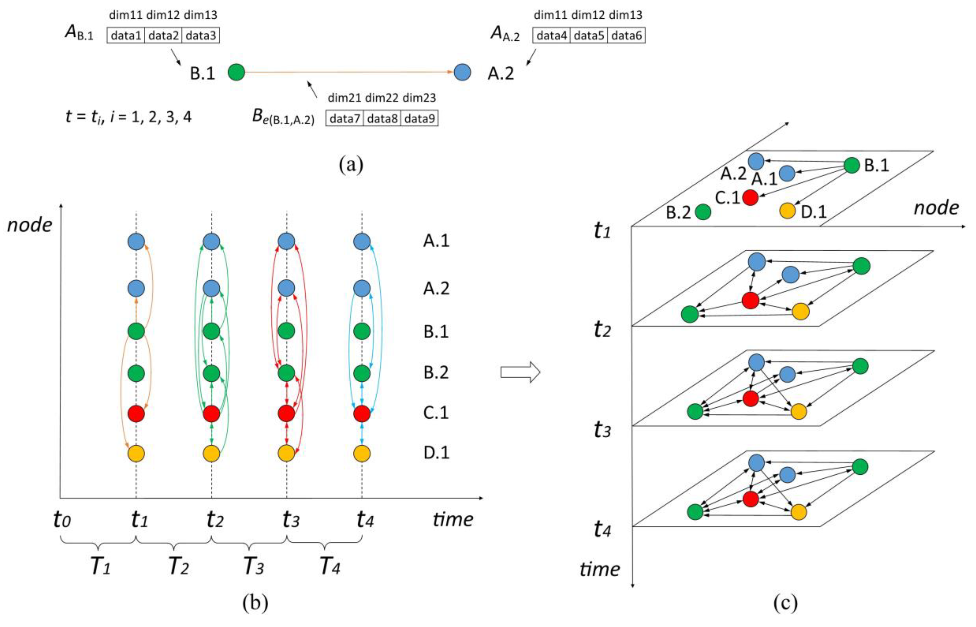
To aid the intuitive understanding of the influence propagation process proposed in this study, we provide a general overview in Figure 1, where an epidemic first outbreaks in instance B.1 and spreads along influential media (infectors) flows within a period of time [t₀, t₄]. Figure 1a shows that instance B.1 exerts influence on instance A.2 until the moment t_i and the cumulative influence can be computed based on a three-dimensional attribute vector $A_{B.1}$ of instance B.1 and vector $B_{e\left(B.1,A.2\right)}$ of directed edge e(B.1, A.2). The digraphs in Figure 1c illustrate all the existing and existed proximity relations and influencing directions of Figure 1b. Detailed definitions and examples are provided next.

Definition 1.

(proximity (P)): Given two instances $o_i$, $o_j$, $f_i$ $\ne$ $f_j$ (their features are distinct), if influential media flow between $o_i$ and $o_j$ within a specific period of time, there exists an association between $o_i$ and $o_j$ called proximity that is denoted as P($o_i$,$o_j$) or P($o_j$,$o_i$). The two instances are called influential instances or a neighbor instance pair and are linked by directed edge(s). A neighbor instance pair indicates the occurrence of influence propagation whose directions are determined by the flows of influential media between the instances. Therefore, two instances of distinct features are proximate whenever two-way edges or a one-way edge link(s) them, regardless of the direction(s) of the edge(s).

Definition 2.

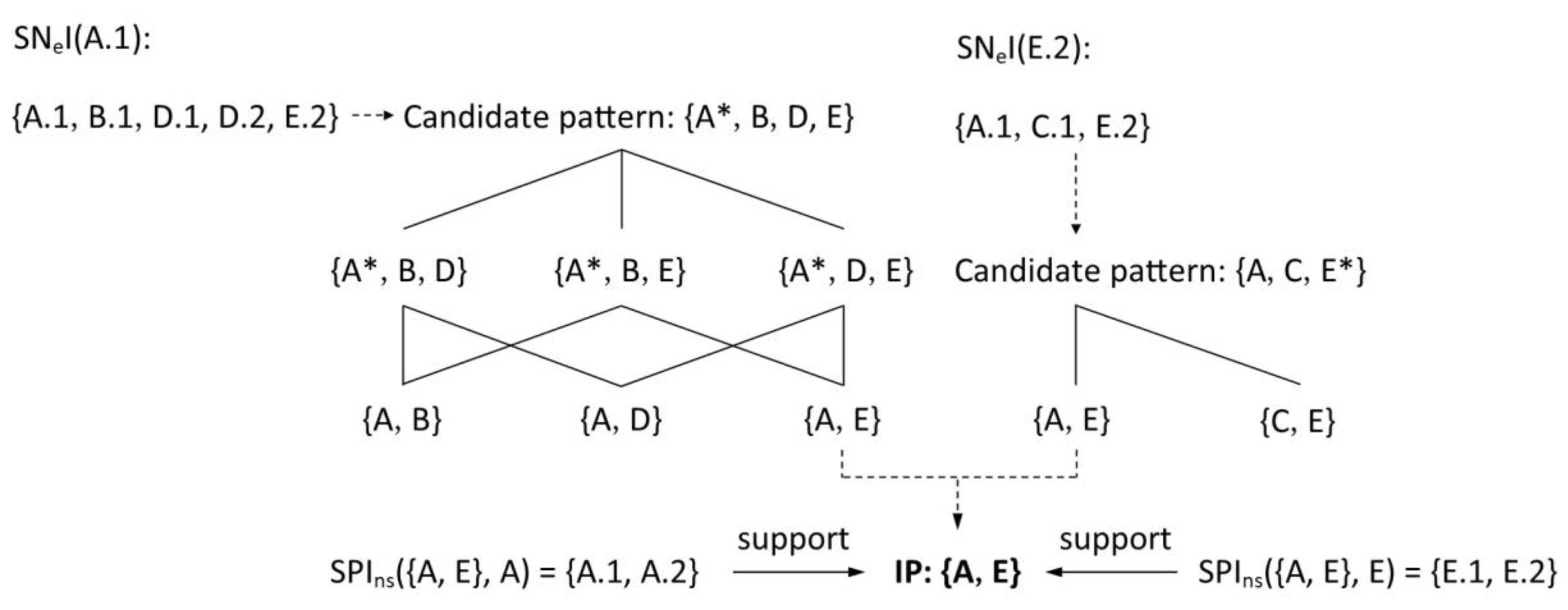
(star neighbor instance set (SN_eI)): Given a spatial instance $o_i$ whose feature is $f_i$ $\in$ F, the SN_eI, i.e., SN_eI($o_i$), denotes a set of instances comprising the central instance $o_i$ and its neighbors with proximity. As depicted in Figure 2, SN_eI(A.1) = {A.1, B.1, D.1, D.2, E.2}.

$${\mathrm{SN}}_{\mathrm{e}}\mathrm{I}(o_i)=\{o_j\in O| o_j=o_i\vee (f_j>f_i\wedge P(o_j, o_i\left)\right)\}$$

(1)

Here, instance $o_j$ corresponds to feature $f_j$ $\in$ F and P refers to a proximate relation; the alphabetic order of features is used for sorting the features to generate non-repetitive SN_eI.

Definition 3.

(candidate pattern (CAP)): Given a star neighbor instance set I = $\left\{o_1,o_2, \dots , o_s\right\}$ whose non-repetitive features form a candidate pattern c, namely:

$$\mathrm{CAP}\left(I\right)={\pi }_{f}I$$

(2)

where ${\pi }_f$ denotes a relational projection operation on features. As depicted in Figure 2, $c$ = {A, B, D, E} is a CAP of SN_eI(A.1).

Definition 4.

(star participation instance (SPI_ns)): Given a candidate pattern c = $\left\{f_1,f_2, \dots , f_k\right\}$, k ≥ 2, feature   $f_{\mathrm{i}}\in$$c,$ and 1 $\le$ i $\le$ k, the star participation instance of feature $f_i$ in pattern c, i.e., SPI_ns(c, $f_i$), denotes an instance set of feature $f_i$ where each instance’s SN_eI contains instances covering all features in c:

$${\mathrm{SPI}}_{\mathrm{ns}}(c, f_i)=\{ o_i| c\subseteq {\pi }_f{\mathrm{SN}}_{\mathrm{e}}\mathrm{I}\left(o_i\right)\}$$

(3)

As depicted in Figure 2, SPI_ns({A, B}, A) = {A.1, A.3}, SPI_ns({A,C,E}, A) = {A.2}.

Definition 5.

(influencing pattern (IP)): Given a candidate pattern c =$\left\{f_1,f_2, \dots , f_k\right\}$, k $\ge$ 2, the pattern c is an IP if any feature $f_i$ $\in$ c, 1 $\le$ i $\le$ k, SPI_ns(c, $f_i$) $\ne \varnothing$.

As depicted in Figure 2, the IPs include seven size-2 ones {{A, B}, {A, C}, {A, D}, {A, E}, {B, C}, {B, D}, {C, E}} and three size-3 ones {{A, B, C}, {A, B, D}, {A, C, E}}.

Definition 6.

(star row instance (SRI)): Given an IP c = $\left\{f_1,f_2, \dots , f_k\right\}$ and one of its star neighbor instance sets, i.e., I = $\left\{o_1,o_2, \dots , o_s\right\}$, k, s $\ge$ 2, then if I is a subset of SN_eI($o_i$) where $o_i$ $\in$ SPI_ns(c, $f_i$), 1 $\le$ i $\le$ s, $f_i$ is the central feature and I (which is called a SRI or SRI(c, $f_i$, $o_i$)) covers c and k = s. The total star row instances of $o_i$ are called SRIs(c, $f_i$, $o_i$). The total star row instances of a central feature $f_i$ in c are called SRI(c, $f_i$). The total SRI(c, $f_i$) of all central features in c constitute star table instance of c, called STI or STI(c).

An instance with an * superscript indicates a central instance in its star row instance. As depicted in Figure 2, SPI_ns({A, B, D}, A) = {A.1, A.3}, SRI({A, B, D}, A, A.1) = {{A.1*, B.1, D.1}, {A.1*, B.1, D.2}}, SRI({A, B, D}, A) = {{A.1*, B.1, D.1}, {A.1*, B.1, D.2}, {A.3*, B.2, D.3}}, STI({A, B, D}) = SRI({A, B, D}, A) + SRI({A, B, D}, B) + SRI({A, B, D}, D) = {{A.1*, B.1, D.1}, {A.1*, B.1, D.2}, {A.3*, B.2, D.3}, {A.3, B.2*, D.2}, {A.1, B.2, D.2*}}.

Since we extracted the time series data from spatio-temporal datasets to reflect the long-term influencing effect of neighbor instances on a central instance in the form of multi-dimensional attributes, it was reasonable to reckon our studied object as an attribute network and utilize its formal expressions. More complicated is that the instances correspond to distinct features, and the edges are also endowed with multi-dimensional attributes in order to distinguish the influencing effect of an instance on neighbor instances of distinct features.

Therefore, what we studied can be denoted as an attributed network G = (F, V, E, $A$), where F denotes the set of features, V denotes the set of nodes (i.e., instances), and E ⊆ (V × V) denotes the set of directed edges in the network. $A\in {ℝ}^{n\times d}$ denotes a matrix that contains all attributes of instances, where n represents the number of instances, d represents the attribute dimension of an instance, and $A_{o_i}\in {ℝ}^d$ represents a row of matrix A; the row means the attribute vector of instance $o_i$. Additionally, we used $B\in {ℝ}^{n^{\prime }\times n^{\prime }\times d^{\prime }}$ to denote a matrix that contains all attributes of edges, where $n^{\prime }$ represents the number of edged instances, $d^{\prime }$ represents the attribute dimension of an edge, and $B_{e_{ij}}\in {ℝ}^{d^{\prime }}$ denotes a row of matrix $B$; the row means the attribute vector of a directed edge $e_{ij}$, which links instances $o_i$ to $o_j$, $f_i \ne f_j$.

Definition 7.

(unilateral influence of instance (UII)): Given a neighbor instance pair $o_i$ and $o_j$, assuming influential media flow from $o_i$ to $o_j$, the instance $o_i$ has influence on $o_j$. The influence UII, i.e., UII($o_i$, $o_j$), is defined as the power of $o_i$ caused its neighbor $o_j$ to change:

$$\mathrm{UII}(o_i, o_j)=(1-p)·A_{o_i}·{\omega }_1^T+p·B_{e_{ij}}·{\omega }_2^T$$

(4)

where p denotes the possibility that instance $o_i$ affects $o_j$, $A_{o_i}$ denotes the attribute vector of instance $o_i$, $B_{e_{ij}}$ denotes the attribute vector of edge $e_{ij}$ between endpoints $o_i$ and $o_j$, and vectors ${\omega }_1^T$ and ${\omega }_2^T$ denote the weights of attributes of instance and edge, respectively.

Example 1.

Choose an instance pair {D.2, A.1} in Figure 2; given $A_{D.2}.$ = [0.819961, 0.102800, 0.774131], ${\omega }_1^T$ = [0.69, 0.23, 0.08]^T, $B_{e\left(D.2,A.1\right)}.$ = [0.611657, 0.238967, 0.582688], ${\omega }_2^T$ = [0.75, 0.07, 0.18]^T, p equals 58%, indicating a percentage that influential media landing instance A.1 takes in the total influential media when moving out of instance D.2. Thus, we obtain UII(D.2, A.1) = (1 − 0.58) $·$ [0.819961, 0.102800, 0.774131] $·$ [0.69, 0.23, 0.08]^T + 0.58 $·$ [0.611657, 0.238967, 0.582688] $·$ [0.75, 0.07, 0.18]^T = 0.610171. In the same way, we can see that UII(B.1, A.1) = 0.840806, UII(D.1, A.1) = 0.189951, as per Formula (4) and the given data.

Definition 8.

(influence of feature in an IP (IFIP)): Given a size-k IP c = $\left\{f_1,f_2, \dots , f_k\right\}$, k $\ge$ 2, feature $f_i\in c$, and the star participation instance SPI_ns(c, $f_i$), the influence of feature $f_i$ in pattern c, i.e., IFIP(c, $f_i$), is defined as sum of maximal influence of SPI_ns(c, $f_i$). The maximal influence of each central instance $o_i$ of SPI_ns(c, $f_i$) denotes the maximum cumulative influence that the instance $o_i$ receives from its neighbor instances in its star row instance SRI(c, $f_i$, $o_i$), namely:

$$\mathrm{IFIP}\left(c,f_i\right)={{\displaystyle \sum }}_{o_i\in {\mathrm{SPI}}_{\mathrm{ns}}\left(c,f_i\right)}\underset{o_i\in SR{I}_s\left(c, f_i, o_i\right)}{\max }\{1-{{\displaystyle \prod }}_{o_j\in \mathrm{SRI}\left(c, f_i, o_i\right),o_j\ne o_i }\left[1-\mathrm{UII}\left(o_j,o_i\right)\right]\}$$

(5)

Example 2.

Given the IP c = {A, B, D} in Figure 2, the UII(B.1, A.1), UII(D.1, A.1), and UII(D.2, A.1) values in example 1 can be used to calculate UII(B.2, A.3) = 0.584771, UII(D.3, A.3) = 0.230016, and SRI(c, A) = {{A.1*, B.1, D.1}, {A.1*, B.1, D.2}, {A.3*, B.2, D.3}}; therefore, IFIP(c, A) = max{[1 − (1 − 0.840806)(1 − 0.189951)], [1 − (1 − 0.840806)(1 − 0.610171)]} + [1 − (1 − 0.584771)(1 − 0.230016)] = max{0.871045, 0.937942} + 0.68028= 1.618222. Formula (5) can ensure that the cumulative influence that a central instance receives from its multiple neighbors grows but does not surpass 1; this arrangement is useful for constructing a metric to evaluate an influencing level of IPs and taking advantage of the downward closure property to prune search space later.

Definition 9.

(star influence ratio (SIR)): Given a size-k IP c = $\left\{f_1,f_2, \dots , f_k\right\}$, k $\ge$ 2, feature $f_i\in c$, and a set containing all the influential instance(s) of feature $f_i$, i.e., $S_{in}(f_i)$, 1 $\le$ i $\le$ k, the ratio SIR, i.e., SIR(c, $f_i$), denotes the average of IFIP(c, $f_i$) on each influential instance of feature $f_i$, namely:

$$\mathrm{SIR}\left(c,f_i\right)=\frac{\mathrm{IFIP}\left(c,f_i\right)}{\left|S_{in}\left(f_i\right)\right|}$$

(6)

where |$S_{in}(f_i)$| denotes the number of influential instances of feature $f_i$.

Definition 10.

(star influence index (SII)): Given a size-k IP c = $\left\{f_1,f_2, \dots , f_k\right\}$, k $\ge$ 2, feature $f_i\in c$, and 1 $\le$ i $\le$ k, the star influence index SII, or SII(c), denotes the minimal star influence ratio SIR(c, $f_i$) among all features in c, namely:

$$\mathrm{SII}\left(c\right)={\min }_{i=1}^k\left\{\mathrm{SIR}\left(c,f_i\right)\right\}$$

(7)

Definition 11.

(high influencing pattern (high IP)): high IP denotes a high influencing pattern if its SII(c) is no less than a given threshold SII_threshold.

Example 3.

For an IP c = {A, B, D} in Figure 2, IFIP(c, A) = 1.618222, IFIP(c, B) = 0.919276, IFIP(c, D) = 0.737827, |S_in(A)| = 3, |S_in(B)| = 2, | S_in(D)| = 3, so SIR(c, A) = 1.618222/3 $\approx$ 0.54, SIR(c, B) $\approx$ 0.46, SIR(c, D) $\approx$ 0.25, SII(c) = min{0.54, 0.46, 0.25} = 0.25. We assumed SII_threshold = 0.2, and since SII(c) > SII_threshold, the IP {A, B, D} is a high IP.

3.2. Problem Statement

Based on the aforementioned analysis, we defined the concerned problem.

Definition 12.

(high influencing pattern discovery in an influence propagation process (HIPD-IPP)): We assumed a nonempty finite set O of spatial instances that belong to a set F of features. If original influence outbreaks in an instance, influential media flow between instances, creating proximate relations between instances of distinct features and showing influencing directions, thus resulting in a set of IPs. Given an influencing measurement SII on star table instances STI of an IP c, the HIPD-IPP problem aims to find the set C of all the IPs whose influencing levels are no less than a given threshold SII_threshold at a specific moment of the influence propagation process, i.e.,:

$$C=\{ c | \mathrm{SII}\left(c\right) \ge {\mathrm{SII}}_{\mathit{threshold}}, c\subseteq F \}$$

(8)

4. Methodology

This method aims to provide a pattern mining tool for an influence propagation process, where the spatial objects have complex interactions. To elaborate this tool, the section is divided into four sub-sections: a framework and Benchmark algorithm, an analysis of related properties, two improved algorithms with pruning strategies, and an analysis of time complexity.

4.1. A Framework and Benchmark Algorithm

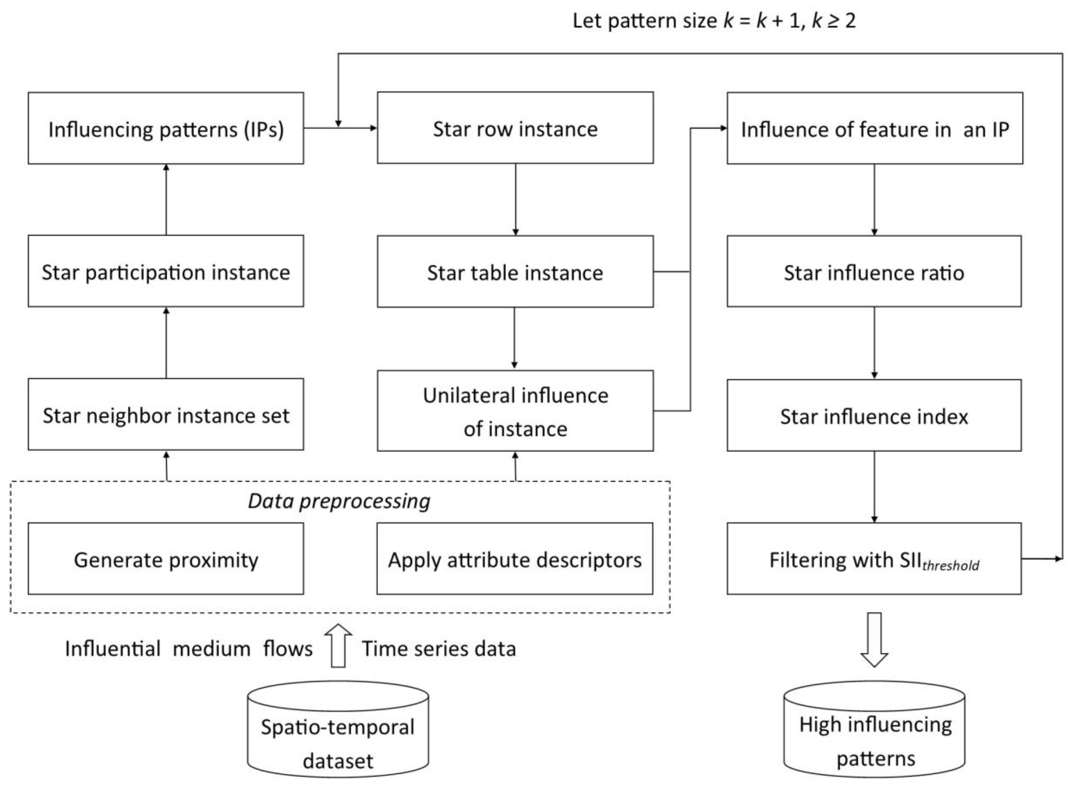
The authors of this study proposed a framework for mining high IPs over time series data (Figure 3) by integrating multidisciplinary knowledge and technologies from fields such as spatial co-location pattern mining, influence analysis, and spatio-temporal pattern discovery.

Specifically, in this framework, a data preprocessing stage is set up before high IP mining, where we first generate proximate relations between instances of distinct features by identifying influential media flows, then apply attribute descriptors to extract time series data and calculate multidimensional attribute vectors for instances and edges, and obtain attribute weights by an analytic hierarchy process. Next, we mine high IPs in two steps: one finds IPs from a star neighbor instance set (in a top-down way), and the other picks up high IPs from the IPs (in a bottom-up way). The details are described as follows.

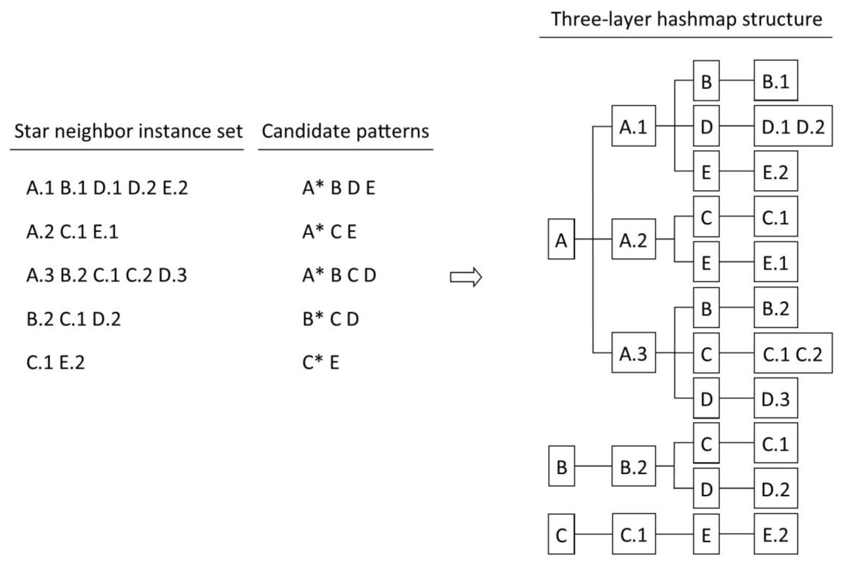
In the first step, one uses a star-shaped materialized model to obtain a star neighbor instance set, and then one identifies candidate patterns and creates a three-layer hashmap structure of HashMap<Character, Map<String, Map<Character, List<String>>>> for fast storage and retrieval. Figure 4 illustrates the process of obtaining a star neighbor instance set, candidate patterns, and a corresponding three-layer hashmap structure from Figure 2. Next, one traverses the candidate patterns to collect qualified patterns to an IPs set or decomposes the unqualified patterns by a central feature to sub candidate patterns at a smaller size (Figure 5). The process iterates size-by-size in a top-down way until it stops at the size-2 level. Finally, the IPs at all sizes can be acquired.

In the second step, one extracts the star table instances, i.e., star row instances of central instances and those of their features for the IPs; then, based on the attribute vectors and attribute weights obtained in the preprocessing stage, one obtains the influence of features in IPs by calculating the sum of the maximum influence of star participation instances of the features in the star row instances. Next, one calculates the star influence ratio and the star influence index for IPs and then filters high IPs with a given SII_threshold. The process starts at size-2 IPs and iterates size-by-size in a bottom-up way until it traverses all IPs. Finally, all the high IPs at all sizes are available.

Based on the aforementioned analysis, we proposed a benchmark algorithm (Benchmark for short) for mining high IPs. The pseudocode is listed in Listing 1 and Listing 2, and the description of Benchmark is as follows.

• Data preprocessing (Steps 1–4): In this step, one extracts time series data from spatio-temporal datasets, identifies each influential instance that has influential media to/from other instances, generates proximate relations for those influential instances (Steps 1–3), and calculates attribute matrices $A$ and $B$, weight vectors ${\omega }_1^T$ and ${\omega }_2^T$, and probabilities p, as described in Section 5.1.3 (Step 4).
• Identifying influencing patterns (Steps 5–12): In this step, one first initiates IPs and HIPs sets and generates a star neighbor instance set as per the proximate relations of instances (Steps 5–6). Then, one applies a three-layer hashmap structure to extract candidate patterns from the star neighbor instance set (Step 7). Next, one generates star row instances and extracts star participation instances (Steps 8–9). Then, one traverses candidate patterns in a top–down way (Step 10) to check whether they are IPs. The identified IPs are added to the IPs set (Step 11); otherwise, the candidate patterns are decomposed with central feature to sub candidate patterns at a smaller size (Step 12).
• Mining high influencing patterns (Steps 13–19): This process starts at size-2 IPs (Step 13). Each c in size-k IPs (Steps 14–15) gets c’s star influence index by calling Function 1 (Step 16). Pattern c, whose SII_c $\ge$ SII_threshold, is then added to HIPs set (Step 17). The while loop continues in ascending order (Step 18). All found HIPs are returned (Step 19).

Listing 1. A benchmark algorithm for high IP mining (Benchmark for short).

Input: $F=\left\{f_1,f_2,\dots ,f_m\right\}$, $O=\left\{o_1,o_2,\dots ,o_n\right\}$, $\left|S_{in}\left(f_i\right)\right|$, SIIthreshold. Output: All high influencing patterns satisfying SIIthreshold. Variables: Please refer to Table A1 in Appendix A.

Data Preprocessing: 1. $\mathrm{For}\mathrm{each}o=\left\{o_1, o_2, \dots , o_s\right\}$ in O, do 2.  If $\forall o_i.$influential_flows != 0, then add $o_i$ to $O_s;$ 3. Generate proximate relations Rs for all influential instances from F and $O_s$ over time series data; 4. Calculate attributes matrices $A$, $B$ for all influencing instances and edges, respectively; compute weight vector ${\omega }_1^T$, ${\omega }_2^T$ for attributes of any instance and edge; and calculate probability vector p. Mining Steps: 5. IPs = $\varnothing$, HIPs = $\varnothing$; 6. Ns = generate_star_neighbor_instance_sets(Rs); 7. Cs = generate_candidate_patterns(Ns); 8. ${\mathrm{SRI}}_{c, f_i}$ = generate_star_table_instance(c, fi, Ns); 9. ${\mathrm{SPI}}_{n{s}_{c,f_i}}$ = extract_star_participation_instance(${\mathrm{STI}}_{c, f_i}$); 10. For each c =$\left\{f_1, f_2, \dots , f_k\right\}$ in Cs do 11.  If $\forall f_i\in$ c, ${\mathrm{SPI}}_{n{s}_{c,f_i}}$ != $\varnothing$, then add c to IPs; 12.   Else decompose c with central feature and add $c^{\prime }$=$\left\{f_1, f_2, \dots , f_{k-1}\right\}$ to Cs; 13. k = 2; 14. While IPsk != $\varnothing$ do 15.  For each c in IPsk, do 16.   ${\mathrm{SII}}_c$ = calculate_star_influence_index(c, Ns, p, A, B, ${\omega }_1^T$, ${\omega }_2^T$); 17.   If ${\mathrm{SII}}_c\ge$ SIIthreshold, then add c to HIPs; 18.  k = k + 1; 19. Return HIPs.

Listing 2. Function 1: calculate_star_influence_index(c, Ns, p, A, B, ${\omega }_1^T$, ${\omega }_2^T$).

Input: c, Ns, p, A, B, ${\omega }_1^T$, ${\omega }_2^T$. Output: Star influence index of pattern c. Variables: Please refer to Table A1 in Appendix A.

For each $f_i$ in c, do  ${\mathrm{IFIP}}_{c,f_i}=$ calculate_central_feature_influence(c, fi, ${\mathrm{SRI}}_{c,f_i}$, ${\mathrm{SPI}}_{n{s}_{c,f_i}}$, p, A, B, ${\omega }_1^T$, ${\omega }_2^T$);  ${\mathrm{SIR}}_{c,f_i}$ = calculate_star_influence_ratio(${\mathrm{IFIP}}_{c,f_i}$, $\left|S_{in}\left(f_i\right)\right|$); ${\mathrm{SII}}_c$ = min ${\mathrm{SIR}}_{c,f_i}$; Return ${\mathrm{SII}}_c$;

4.2. Analysis of Related Properties

As the Benchmark needs to traverse all IPs size-by-size to mine high IPs, it is inefficient at treating large-scale data, so we found ways to improve its efficiency. In co-location pattern mining research, a downward closure property (also called anti-monotonicity), i.e., a measurement of pattern that continually decreases with the rise of pattern size, is often applied to prune patterns whose measurement are less than a given threshold. Unfortunately, as in Figure 2, SII({A, B}) = 0.15 < SII({A, B, D}) = 0.25, so the IPs measured with star influence index cannot satisfy this property. As such, it was necessary to find other ways to boost efficiency.

Lemma 1.

(upper bound of $\mathit{SII}$ satisfies downward closure property): the measurement of the star influence index has an upper bound that satisfies the downward closure property.

Proof. 

please refer to proof B2 for Lemma 1 in Appendix B.□

As mentioned in Lemma 1, the $\mathrm{SII}\left(c\right)$’s upper bound $\mathrm{SPI}\left(c\right)$ = $mi{n}_{i=1}^k\left\{\frac{\left| SPIns\left(c, f_i\right) \right|}{\left|S_{in}\left(f_i\right)\right|}\right\}$ satisfies the downward closure property, that is, for a size-k IP $c$ and a k + 1-size IP $c^{\prime }$ = $c{\displaystyle \cup }${$f_{k+1}$}, k $\ge$ 2 and $\mathrm{SPI}\left(c^{\prime }\right)\le \mathrm{SPI}\left(c\right)$, so when $\mathrm{SPI}\left(c\right)$ < SII_threshold, there exists $\mathrm{SII}\left(c^{\prime }\right)\le \mathrm{SPI}\left(c^{\prime }\right)\le \mathrm{SPI}\left(c\right)$ < SII_threshold and $\mathrm{SII}\left(c\right)\le \mathrm{SPI}\left(c\right)$< SII_threshold. Therefore, the IP c and all its super IPs $c^{\prime }$ are not high influencing patterns and should be pruned.

This is the case for pruning IPs c whose $\mathrm{SPI}\left(c\right)$ < SII_threshold. Once $\mathrm{SPI}\left(c\right)\ge \mathrm{SII}$_threshold, so we needed to find another pruning strategy. Inspired by Definition 10 that $\mathrm{SII}$(c) takes the minimum $\mathrm{SIR}$(c, $f_i$), we proposed one more lemma for designing a pruning strategy as follows.

Lemma 2.

(an incremental feature determines the influencing level of super IP of a high IP): Given a size-k high IP c = $\left\{f_1,{ f}_2, \dots ,{ f}_k\right\}$, $f_i\in c$, k $\ge$ 2, and its super IP $c^{\prime }$ = $c{\displaystyle \cup }\left\{f_l\right\}$, once SRI(c, $f_i$) = SRI($c^{\prime }$, $f_i$), $f_i\ne f_l$, the influencing level of $c^{\prime }$ depends on whether the value of star influence ratio $\mathrm{SIR}$($c^{\prime }$, $f_l$) is no less than $\mathrm{SII}$_threshold.

Proof. 

please refer to proof B3 for Lemma 2 in Appendix B.□

As mentioned in Lemma 2, once $\mathrm{SII}\left(c\right)\ge \mathrm{SII}$_threshold and $\mathrm{SRI}$(c, $f_i$) $\subseteq$ $\mathrm{SRI}$($c^{\prime }$, $f_i$), $f_i\ne f_l$, when $\mathrm{SIR}$($c^{\prime }$, $f_l$)$\ge \mathrm{SII}$_threshold, $\mathrm{SII}\left(c^{\prime }\right)\ge \mathrm{SII}$_threshold holds; otherwise, $\mathrm{SII}\left(c^{\prime }\right)<\mathrm{SII}$_threshold, so an incremental feature $f_l$ can be used to judge the influencing level of a supper IP $c^{\prime }$ of a high IP c.

Therefore, the authors of this study can propose two pruning strategies as per Lemmas 1 and 2 and put forward two accordingly improved algorithms to boost efficiency.

4.3. Two Improved Algorithms with Pruning Strategies

In view of Lemma 1, indicating that an IP c = $\left\{f_1,f_2, \dots , f_k\right\}$, k $\ge$ 2, feature $f_i\in c$, and all its super IPs can be pruned whenever SPI(c) = ${\min }_{i=1}^k\left\{\left|{ \mathrm{SPI}}_{\mathrm{ns}}\left(c, f_i\right) \right|/\left|S_{in}\left(f_i\right)\right|\right\}$ < SII_threshold, we introduced an improved algorithm (Improved-1 for short) for mining high IPs with a pruning strategy, as depicted in Listing 3. Improved-1 accepts codes of Benchmark and inserts additional codes between Steps 12 and 13 of Benchmark. Thus, Steps 13–19 of Benchmark are Steps 19–25 of Improved-1.

Listing 3. Improved algorithm for high IP mining with a pruning strategy (Improved-1 for short).

Input, Output, Variables: The same as in Listing 1.

13 k = 2; 14 $\mathrm{While} {\mathrm{IPs}}_k !=\varnothing$, do 15  For each c in IPsk, do 16   ${\mathrm{SPI}}_c$$=\mathrm{compute}\text{\_}\mathrm{upper}\text{\_}\mathrm{bound}\text{\_}\mathrm{index}({\mathrm{SPI}}_{{\mathit{ns}}_{c,f_i}}$$, \left|S_{in}\left(f_i\right)\right|);$ 17   $\mathrm{If} {\mathrm{SPI}}_c < {\mathrm{SII}}_{\mathit{threshold}}, \mathrm{then} \mathrm{prune} c \mathrm{and} \mathrm{all} \mathrm{its} \mathrm{super} \mathrm{IPs} \mathrm{in} \mathrm{IPs};$ 18  k = k + 1;

Whenever $\mathrm{SPI}$(c) $\ge \mathrm{SII}$_threshold, one cannot again use upper bounds to prune low IPs. Lemma 2 provides a concise way to identify high IPs from size-k IPs (k > 2) based on size-2 high IPs, i.e., first filter size-2 high IPs and then search their super IPs $c^{\prime }$ = $c{\displaystyle \cup }\left\{f_l\right\}$ in IPs size by size. Once $c^{\prime }$ exists and $\mathrm{SRI}$($c$, $f_i$) $\subseteq \mathrm{SRI}$($c^{\prime }$, $f_i$), a common case occurs among low-size IPs, and the value of $\mathrm{SIR}$($c^{\prime }$, $f_l$) determines whether $c^{\prime }$ is a high IP or not. IPs with $\mathrm{SIR}$($c^{\prime }$, $f_l$) $\ge$ SII_threshold are added to HIPs; otherwise, they are pruned. As for other cases, such as when IPs are not super IPs of a high IP or $\mathrm{SRI}$($c$, $f_i$) $\supset \mathrm{SRI}$($c^{\prime }$, $f_i$), the regular calculation of the features of an IP should be conducted to identify high IPs. The iteration proceeds until IPs is traversed.

Therefore, we proposed another improved algorithm (Improved-2 for short) for mining high IPs with two pruning strategies, as depicted in Listing 4. Improved-2 accepts codes (Steps 1–18) of Improved-1 and replaces Steps 19–25 of Improved-1 with the following codes (Steps 19–42 in Listing 4).

Listing 4. Improved algorithm for high IP mining with two pruning strategies (Improved-2 for short).

Input, Output, Variables: The same as in Listing 1.

19 While IPs2 != $\varnothing$, do 20  For each c in IPs2, do 21   ${\mathrm{SII}}_c$ = calculate_star_influence_index(c, Ns, p, A, B, ${\omega }_1^T$, ${\omega }_2^T$); 22   If ${\mathrm{SII}}_c\ge$ SIIthreshold, then add c to HIPs; 23 k = 3; 24  While IPsk != $\varnothing$ do 25  For each $c^{\prime }$ in IPsk, do 26   If HIPsk-1 != $\varnothing$, then do 27    If $c^{\prime }$ finds a sub pattern c in HIPsk-1, then do    // suppose $c^{\prime }$= $c{\displaystyle \cup }{f}_l$ 28     If ${\mathrm{SRI}}_{c,f_i} \subseteq { \mathrm{SRI}}_{c^{\prime },f_i}$ then do 29        ${\mathrm{IFIP}}_{c^{\prime },f_l }$ = calculate_star_feature_influence($c^{\prime }$, $f_l$, ${\mathrm{SRI}}_{c^{\prime },f_l}$, ${\mathrm{SPI}}_{{\mathrm{ns}}_{c^{\prime },f_l}}$, p, A, B, ${\omega }_1^T$, ${\omega }_2^T$); 30       ${\mathrm{SIR}}_{c^{\prime },f_l}$ = calculate_star_influence_ratio(${\mathrm{IFIP}}_{c^{\prime },f_l }$, $\left|S_{in}\left(f_l\right)\right|$); 31       If ${\mathrm{SIR}}_{c^{\prime },f_l}\ge$ SIIthreshold, then add $c^{\prime }$ to HIPs; 32     Else do 33       ${\mathrm{SII}}_{c^{\prime }}$ = calculate_star_influence_index($c^{\prime }$, Ns, p, A, B, ${\omega }_1^T$, ${\omega }_2^T$); 34       If ${\mathrm{SII}}_{c^{\prime }}\ge$ SIIthreshold, then add $c^{\prime }$ to HIPs; 35    Else do 36      ${\mathrm{SII}}_{c^{\prime }}$ = calculate_star_influence_index($c^{\prime }$, Ns, p, A, B, ${\omega }_1^T$, ${\omega }_2^T$); 37      if ${\mathrm{SII}}_{c^{\prime }}\ge$ SIIthreshold, then add $c^{\prime }$ to HIPs; 38   Else do 39    ${\mathrm{SII}}_{c^{\prime }}$ = calculate_star_influence_index($c^{\prime }$, Ns, p, A, B, ${\omega }_1^T$, ${\omega }_2^T$); 40    If ${\mathrm{SII}}_{c^{\prime }}\ge$ SIIthreshold, then add $c^{\prime }$ to HIPs; 41  k = k + 1; 42 Return HIPs.

4.4. Analysis of Time Complexity

To analyze the time complexity of the high IP mining algorithms based on Benchmark, we divided the whole process into four relatively independent parts, proximity generation, IPs search, size-2 high IP mining, and size-k (k > 2) high IP mining, and formulated an equation for total time cost $T$:

$$T=T_{generate\_P}\left(S\right)+T_{IPs\_search}\left(P\right)+T\left(2\right)+{{\displaystyle \sum }}_{k>2}T\left(k\right)$$

(9)

where S denotes the input data sources, P denotes all proximity relations, and $T\left(2\right)$ denotes time cost for size-2 high IP mining. For the sake of discussion, u denotes the amount of influential instances at the last moment of a specified period, m denotes total feature amount, and n denotes total instance amount in space.

$T_{generate\_P}\left(S\right)$: first of all, one searches influential medium flows existing between influential instances of distinct features to find neighbor instance pairs; one search costs O(1) and proximity relations are O(u²) at most, so $T_{generate\_P}\left(S\right)$ = O(u²).

$T_{IPs\_search}\left(P\right)$: An influential instance has at most u neighbors, so after traversing the influential instances and their neighbors and applying a three-layer hashmap structure to store the instances and their candidate patterns, star neighbor instance sets cost time O(u²). Suppose the largest size of candidate patterns to be a (2 $\le$ a $\le$ m); as single feature patterns are not in consideration, total candidate patterns are $2^a$ − m − 1. A candidate pattern is moved to an IPs set or be decomposed with a central feature to sub candidate patterns at a smaller size. In the worst case, this process costs time O(u²) + O($(2^a$ − m − 1)$·$u).

$T\left(2\right)$: The size-2 IPs are traversed to mine high IPs. Due to the design of the three-layer hashmap structure, inquiring star row instances of a size-2 IP costs $T{\left(2\right)}_1$ = O(1). Considering the worst case, each central instance of a size-2 IP has u-1 neighbor instances of distinct feature of the pattern. The time to calculate $\mathrm{IFIP}\left(c,f_i\right)$ is $T{\left(2\right)}_2$ = u$·$m$·$O(1) = O(u$·$m), and calculations of SIR and SII cost $T{\left(2\right)}_3$ = O($m)$. As $\left|S_{in}\left(f_i\right)\right|$ is a constant, size-2 IPs counts $C_m^2$ as the upmost; therefore, $T\left(2\right)$ = $C_m^2·$[$T{\left(2\right)}_1$+$T{\left(2\right)}_2$+$T{\left(2\right)}_3$] = $C_m^2·[$O(1) + O(u$·$m) + O($m))$] = O(u$·$m³).

${\displaystyle \sum }_{k>2}T\left(k\right)$: As discussed above, candidate IPs for mining high IPs count $2^a$ − $C_m^2$ − m − 1 and the time to mine a high IP with SII metric costs O(u$·$m), so the time cost of ${\displaystyle \sum }_{k>2}T\left(k\right)$ is O($2^a$ − $C_m^2$ − m − 1)$·$O(u$·$m).

In summary, in the worst case, total time consumption $T$ in Benchmark costs:

$$T=O\left(u^2\right)+O\left(u^2\right)+O\left(\right(2^a - m - 1)·u)+O(u·m^3)+O(2^a - C_m^2 - m - 1)·O(u·m)=O\left(u^2\right)+O\left(u{m}^3\right)+O(2^a·u·m)$$

(10)

The heuristic strategy, i.e., identifying influential instances out of space, creates only partial instances that need to be processed, and the two improved algorithms, i.e., Improved-1 and Improved-2, limit the value of a within a finite range. As such, our method is related to the amount of influential media and features and the maximum of pattern size, but it is not related to the amount of instances. Its operation speed is fast, especially in the early and middle stages of influence propagation. However, its effects on cost saving are uncertain due to the unknown scale and distribution properties of datasets.

5. Experimental Evaluation

In this section, we provide experimental results and corresponding analysis, including the experimental conditions, data description and preprocessing, effectiveness of high IP mining algorithms on a real dataset, efficiencies of high IP mining algorithms on a real dataset and a synthetic dataset, and the scalability of high IP mining algorithms on the synthetic datasets. Java 1.8.0_202, Java SE (build 1.8.0_202-b08), Java Server VM (build 25.202-b08, mixed mode), and Eclipse IDE 2019-03(4.11.0) were used to run experiments on a normal PC with Intel core i7-8700K CPU @ 3.70 GHz, 3.70 GHz, 16.0 GB RAM, Windows 10 Pro (64-bit).

5.1. Study Area and Data

5.1.1. Study Area

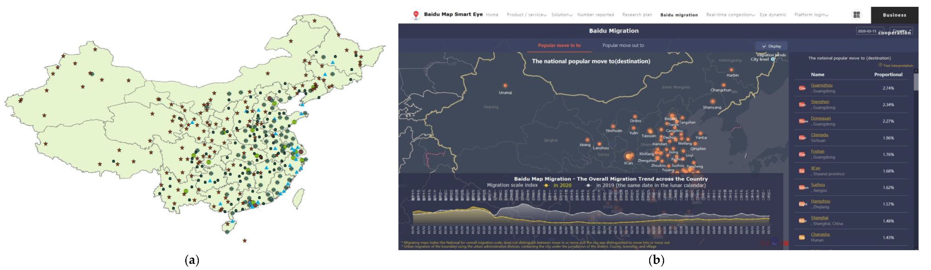
Mainland China was the study area. Hong Kong, Macao, and Taiwan were excluded due to their distinct enforcement of epidemics prevention and control measures. With reference to the 2019 China cities classification of China Business News, we enumerated 365 cities of China (Figure 6a) comprising 304 cities in 22 provinces, 57 cities in 5 autonomous regions, and 4 municipalities. Each city refers to an administrative area that comprises affiliated cities and counties.

5.1.2. Data Description

Though the influence propagation process proposed in this work was specifically designed for epidemic dispersal scenarios, as far as we know, no such public dataset is currently available. Therefore, we created a real dataset, Real-1, by collecting data on COVID-19 epidemic dispersal, urban statistics, and ambient conditions for all the cities in mainland China.

Our epidemic dispersal data, supplemented and verified by Doctor Clove, included the number of infections, the number of cures, and the number of deaths in all cities from 12 December 2019 to 16 July 2020, and the number of inter-city infector migrations; they were downloaded from the COVID-19/2019-nCoV time series infection data warehouse, the COVID-19 data repository by the Center for Systems Science and Engineering (CSSE) at Johns Hopkins University, the epidemic announcements of the National Health Commission of China, and its provincial and municipal affiliates. These data were used in this study to calculate the attribute vectors of cities (i.e., infected ratio, non-cured ratio, and death ratio), and to determine proximate relations between cities (i.e., instances) of distinct categories (i.e., features). Urban statistics included the aforementioned China cities classification of China Business News on 26 May 2019 and the inter-city human migration data and intra-city traffic intensity data from 12 December 2019 to 16 July 2020; these data were downloaded from Baidu Map Smart Eye site (Figure 6b), and they were used to classify all the cities into seven categories of {A, B, …, G} and to describe human-flow closeness and traffic intensity similarities between neighbor instance pairs. Ambient condition data included daily average values of relative humidity during 1960–2017; ultraviolet radiation index values during 1961–2014; and temperature, precipitation, and overall air quality index values during 1981–2010 for all cities. These data were downloaded from the Science Data Bank and China Meteorological Observatory, and they were used to calculate the ambient condition similarities between neighbor instances.

In addition, we used a spatial data synthesizer similar to that used in [17,19,23] to generate 18 synthetic datasets at distinct scales (i.e., Syn-1~18).

A summary of real and synthetic datasets is presented in

Table 1. A summary of real and synthetic datasets.

Name of Dataset	Instance Amount	Influential Media Amount	Feature Amount	Attribute Dimensions
Real-1	365	1,300	7	6
Syn-1	20,000	5,000	15	6
Syn-2/3/4/5/6	200,000/400,000/600,000/ 800,000/1,000,000	10,000	20	10
Syn-2/7/8/9/10	200,000	10,000/20,000/30,000/40,000/50,000	20	10
Syn-2/11/12/13/14	200,000	10,000	20/30/40/50/60	10
Syn-2/15/16/17/18	200,000	10,000	20	10/20/30/40/50

.

5.1.3. Data Preprocessing

The data preprocessing of the Real-1 dataset can be described as follows.

Generate proximate relations: we created semantic proximities for neighbor instance pairs once they interacted via flows of influential media.

Obtain attribute vectors: As an influence propagation process usually shows different properties within distinct time segments of a consecutive period of time, we divided the time span of the Real-1 dataset, i.e., from 12 December 2019 to 16 July 2020, into five time segments by four points in time, i.e., January 24, February 8, March 13, and April 30 of 2020. Accordingly, we designed a new attribute descriptor to obtain attribute vectors by extracting time series data from the Real-1 dataset, preprocessing them in the divided time segments, and integrating them.

Definition 13.

(Attribute Descriptor, AD): The descriptor AD denotes an integrated operation on attributes of an object within a specific period of time T = {$T_1$, $T_2$, …, $T_l$} that is used to measure the negative influence between two instances of distinct features.

When an object denotes an influencing instance $o$, the descriptor AD produces the attribute vector $A_o$, i.e., AD(o), for the instance $o$ as follows:

$$\mathrm{AD}\left(o\right)=[N_{orm}\left(D_s\left(o, v_1, T\right)\right),N_{orm}\left(D_s\left(o, v_2, T\right)\right),\dots , N_{orm}\left(D_s\left(o, v_w, T\right)\right)]$$

(11)

where $v_j\in$ V = {$v_1$,$v_2$,…$v_w$} denotes a dimensional attribute of instance $o$, $T_i\in$ T denotes a time segment of T, $D_s$ averages the cumulative values $o{\left[v_j\right]}_{T_i}$ of attribute $v_j$ of instance $o$ in segment $T_i$ (i.e., $D_s\left(o,v_j, T\right)$ = ${\displaystyle \sum }_{i=1}^{l}o{\left[v_j\right]}_{T_i}/l$), and $N_{orm}$ denotes a min–max normalization of the value of $D_s$. For Formula (11), l = 5, w = 3, $v_1$ denotes the infected ratio, $v_2$ denotes the non-cured ratio, and $v_3$ denotes the death ratio; therefore, the AD(o) is a three-dimensional attribute vector with values processed with the three kinds of ratios.

When an object denotes a directed edge $e$, the descriptor AD produces the attribute vector $B_e$, i.e., AD($e$), for edge $e$ as follows:

$$\mathrm{AD}\left(e\right)=[N_{orm}\left(D_h\left(e, T\right)\right),N_{orm}\left(D_c\left(e, V_1^{\prime },V_1^{″}, T\right)\right), \dots ,N_{orm}\left(D_c\left(e, V_z^{\prime }, V_z^{″}, T\right)\right]$$

(12)

where $D_h$ averages the modulus for the vector sum of media flowing in two opposite directions in edge $e$ within T, i.e., $D_h\left(e, T\right)$ = ${\displaystyle \sum }_{i=1}^l{\{{\left(r_{pq}^{T_i}/\left|T_i\right|\right)}^2+{\left(r_{qp}^{T_i}/\left|T_i\right|\right)}^2\}}^{1/2}/l$, supposing the edge e has two endpoints $o_p$, $o_q$; $f_p$ $\ne$ $f_q$; $r_{pq}^{T_i}$ denotes the amount of media moving from $o_p$ to $o_q$ within a time segment $T_i\in$ T; $r_{qp}^{T_i}$ denotes the amount of media moving in the opposite direction within the same segment $T_i$; and $\left|T_i\right|$ denotes the number (i.e., days) of $T_i$. Additionally, $D_c$ operates cosine similarity between an attribute vector $V_i^{\prime }$ = {$v_1^{\prime }$,$v_2^{\prime }$,…$v_{w’}^{\prime }$} of endpoint $o_p$ and another attribute vector $V_i^{″}$ = {$v_1^{″}$,$v_2^{″}$,…$v_{w’’}^{″}$} of endpoint $o_q$ within T, $v_i^{\prime }$ (or $v_i^{″}$) denotes a dimensional value for vector $V_i^{\prime }$ (or $V_i^{″}$), and $N_{orm}$ denotes a min-max normalization. For Formula (12), l = w‘= w‘’ = 5, and z = 2; $D_h\left(e, T\right)$ processes media (i.e., human-flow) data; $D_c\left(e, V_1^{\prime },V_1^{″}, T\right)$ processes the daily averaged ambient condition data of relative humidity, ultraviolet radiation index, temperature, precipitation, and overall air quality index; and $D_c\left(e, V_2^{\prime },V_2^{″}, T\right)$ processes daily averaged inner-city traffic intensity data within five divided time segments of T. Therefore, AD(e) is a three-dimensional attribute vector with processed values of human-flow closeness, ambient conditions, and inner-city traffic intensity.

Calculate weights of attributes: We applied an analytic hierarchy process, a widely applied approach introduced by Thomas L. Saaty [49] for quantifying the weights of decision criteria and evaluating relative magnitudes of objects through pairwise comparisons, to calculate the attribute weights for instances and edges. The process can be described as follows. A nine-rank metric standard is first introduced to artificially assign weights to paired attributes to obtain a judgment matrix. Then by normalizing the column vector and doing an arithmetic average of the row vector, three attribute weight matrices for instances (or edges) can be obtained. Next, after a consistency check, one can endow the attributes of instances (i.e., ${\omega }_1^T$) with three weights, infected ratio (0.69), non-cured ratio (0.23), and death ratio (0.08), and can endow the attributes of edges (i.e., ${\omega }_2^T$) with another three weights: human-flow closeness (0.75), ambient condition (0.07), and inner-city traffic intensity (0.18).

Calculate the possibility of influence for a neighbor instance pair: The possibility p that instance $o_i$ affects its neighbor instance $o_j$ can be calculated as a percentage of the amount of influential media leaving $o_i$ for $o_j$ occupies the total influential media leaving $o_i$.

Therefore, one can obtain attribute matrices $A$ and $B$, weight vectors ${\omega }_1^T$ and ${\omega }_2^T$, and probability vector p from spatio-temporal datasets in the data preprocessing stage; then, one is ready for influence evaluation between neighbor instances.

The data preprocessing of the synthetic datasets can be described as follows.

Generate random numbers for influential media: Based on synthetic datasets, one generates random numbers of influential media in [1, 2] for influencing instances and generates random numbers of influential media in [10, 15] for influenced instances; the generated numbers are randomly assigned to instances in a distributed manner as much as possible at five specific moments. The amount of influential media in influencing instances equals that of influential media in influenced instances at adjacent moments, and the total amount of influential media is specified for a specific synthetic dataset, e.g., five thousand influential media are generated for the Syn-1 dataset. Then, those influential media flow in a random way from influencing instances to the influenced instances at those moments. Accordingly, proximate relations between influential instances of distinct features can be obtained.

Generate random numbers for attributes: one generates random numbers in [0, 1) for attributes of instances (or edges) as required during the running process of high IP mining algorithms over synthetic data.

5.2. Effectiveness of High IP Mining Algorithms

We were the first to introduce high IP mining for an influence propagation process, so we chose the most similar high influence co-location pattern mining algorithm [28] (HICP mining for short) for a comparison of effectiveness and efficiency.

Our comparison of effectiveness was based on the Real-1 dataset with preset variables as default unless specified otherwise. When studying the effect of the distance threshold on pattern amount, we set SII_threshold = InI_threshold = 0.01 and the distance threshold R took values within [100, 500] km. When studying the effect of SII_threshold/InI_threshold on pattern amount, we set R = 500 km and the influence index threshold SII_threshold/InI_threshold took values within [0.01, 0.03].

Please note that to facilitate the comparison of the effectiveness and efficiencies of the two algorithms in the same orders of magnitude in Section 5.2 and Section 5.3, we temporarily replaced the denominator $|S_{in}(f_i\left)\right|$ of Formula (6) with $|S(f_i\left)\right|$ (which denotes the number of instances of feature $f_i)$ for high IP mining. Because $|S_{in}(f_i\left)\right|$ $\le |S(f_i\left)\right|$, the properties and codes of the high IP mining algorithms are not affected.

5.2.1. Comparison of Top 5 Patterns at All Sizes Mined by Benchmark and HICP Mining of the Real-1 Dataset

Table 2. Top 5 patterns of high IP and HICP (marked with influence index values).

	Size-2 Patterns	Size-3 Patterns	Size-4 Patterns	Size-5 Patterns
Top 5 high influencing patterns (mined by Benchmark)	{E,F} 0.036990 {D,E} 0.035215 {F,G} 0.019201	{B,D,E} 0.155312 {B,E,F} 0.089215 {C,E,F} 0.025089 {D,E,F} 0.021476 {C,D,F} 0.017934	{A,B,C,D} 0.068126 {B,C,D,E} 0.047151 {B,C,E,F} 0.013266	{A,B,C,D,E} 0.01
Top 5 high influence co-location patterns (mined by HICP mining)	{F,G} 0.019537 {E,F} 0.015028 {C,F} 0.014729 {D,F} 0.013853 {C,D} 0.013547	{C,E,F} 0.012839 {C,D,F} 0.012581 {D,E,F} 0.011468 {D,F,G} 0.011316 {C,D,E} 0.010995	{C,D,E,F} 0.010517	null

Please note that Benchmark is the basic algorithm for realizing the high IP mining framework; HICP mining denotes high influence co-location pattern mining.

reveals that Benchmark can find more patterns than the HICP mining algorithm, i.e., a size-2 pattern {D, E}, two size-3 patterns {{B, D, E}, {B, E, F}}, three size-4 patterns {{A, B, C, D}, {B, C, D, E}, {B, C, E, F}}, and a size-5 pattern {A, B, C, D, E}. That is because HICP mining can only find high influence co-location patterns whose table instances exist in R-bounded cliques, while Benchmark can find high IPs beyond the stretch of distance threshold R. Additionally, the two algorithms found some common patterns, i.e., two size-2 patterns {{E, F}, {F, G}} and three size-3 patterns {{C, E, F}, {D, E, F}, {C, D, F}}, because compared with remote cities, adjacent cities more frequently exchange influential media.

The results showed that the influence index of HICP satisfied the downward closure property but the star influence index of high IP did not, e.g., InI{C, E, F} = 0.012839, while InI{C, E} = 0.013159, InI{C, F} = 0.014729, InI{E, F} = 0.015028, InI{C, E, F} < min{InI{C, E}, InI{C, F}, InI{E, F}}. On the other hand, the high IP {B, C, D, E} had no sub high IP {B, C}, and SII{D, E} = 0.035215, while SII{B, C, D, E} = 0.047151.

The authors of this study classified several cities with serious epidemics into feature B and found high IPs containing feature B at size-3 and above, while the HICP mining found no HICPs with feature B at all sizes. This was because high IP mining relies on influential medium flows, regardless of spatial distance, and star table instances of IPs appear in a star structure that is more common than table instances of co-locations in cliques. Additionally, this shows that the provincial capital cities (categorized into feature B) and regional central cities (categorized into feature C) both have stronger influences than ordinary cities (categorized into feature D) on relatively remote cities (categorized into features E, F, and G), and cities at higher rank have wider influence due to the cumulative effects of influence propagation. The results illustrated that the framework and algorithms proposed in this study are practical and feasible for high IP discovery in an influence propagation process.

5.2.2. Comparison of Mined Results of Benchmark and HICP Mining of the Real-1 Dataset

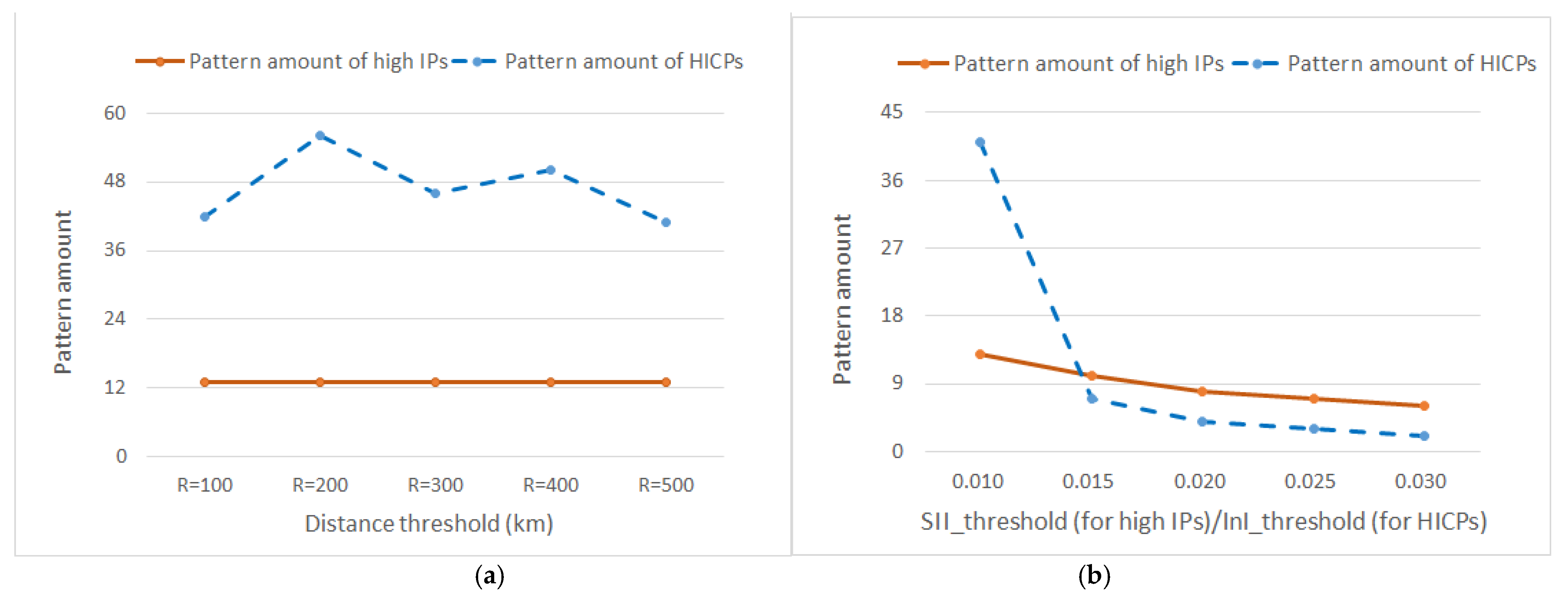
• Effect of distance threshold on pattern amount

Figure 7a shows that as R rose within [100, 500] km, the amount of high IPs (orange solid line) remained 13 while the amount of HICPs (blue dashed line) fluctuated within a numerical range of [41, 56]. This was because Benchmark mined high IPs based on influential medium flows, regardless of R-constrained spatial distances. However, HICP mining discovered more neighbor instance pairs with the rise of R. In addition to new instance pairs, existing instances may have had more neighbors and the sizes of candidate patterns may have been larger. The influence index metric designed for high influence co-location pattern took the minimum among influence ratios of features and satisfied the downward closure property, and the influences of instances mainly depended on the attribute similarity entropy, the values of which were uncertain. Therefore, the pattern amount mined by HICP mining fluctuated as the distance threshold increased.

• Effect of SII_threshold/InI_threshold on pattern amount

Figure 7b shows that when SII_threshold/InI_threshold rose within [0.01, 0.03], the amount of high IPs (orange solid line) gradually declined from 13 at SII_threshold = 0.01 to 6 at SII_threshold = 0.03. On the other hand, the amount of HICPs (blue dashed line) sharply declined from 41 at InI_threshold = 0.01 to 7 at InI_threshold = 0.015 and then slowly descended to 2 at InI_threshold = 0.03. This shows that the amount of patterns decreased as SII_threshold/InI_threshold rose, the majority of the HICPs had lower influence levels, and the high IPs had a wider variety of influence levels.

5.3. Efficiencies of High IP Mining Algorithms

Experiments were conducted to compare the efficiencies of the high IP mining and HICP mining by using two kinds of thresholds (i.e., distance threshold and influence index threshold) over the Real-1 and Syn-1 datasets. Because the high IP mining algorithms apply principles for generating neighbor instance pairs different from those of HICP mining, the latter spends more time finding neighbor pairs by calculating their spatial distance; therefore, we deducted such neighbor generation time during the efficiency comparison.

The comparison of efficiency was preset with variables as default unless specified otherwise. When studying the effect of distance threshold on efficiency, we set SII_threshold = InI_threshold = 0.01 and the distance threshold R took values within [100, 500] km (on the Real-1 dataset) or within [80, 400] (on the Syn-1 dataset). When studying the effect of SII_threshold/InI_threshold on efficiency, we set R = 500 km (on the Real-1 dataset) or R = 400 (on the Syn-1 dataset) and the influence index threshold SII_threshold/InI_threshold took values within [0.01, 0.03].

5.3.1. Efficiency Comparison of High IP and HICP Mining Algorithms over the Real-1 Dataset

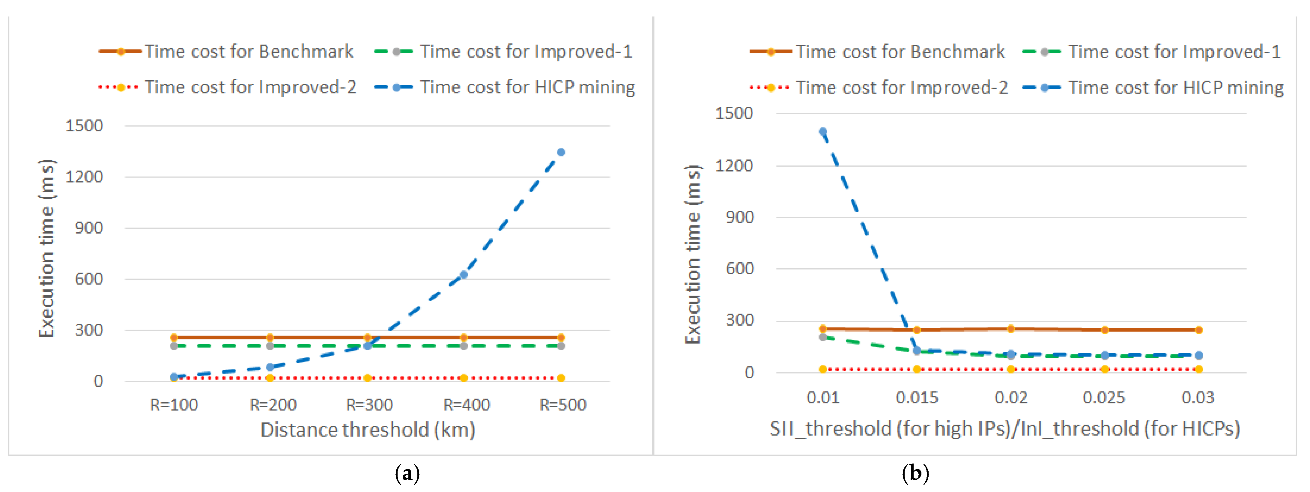
• Effect of distance threshold on efficiency

Figure 8a reveals that the time costs of the high IP mining algorithms were 258, 206, and 20 ms, and Improved-2 ran faster than the HICP mining algorithm at all times. On the other hand, the time cost of the HICP mining algorithm (blue dashed line) grew with the rise of the distance threshold; it started at 29 ms at R = 100 km, passes 209 ms at R = 300 km, and reached 1347 ms at R = 500 km. This was because the HICP mining relied on distance thresholds and needed more time to process incremental neighbor instance pairs with the rise of R, while the high IP mining algorithms did not depend on distance thresholds.

• Effect of SII_threshold/InI_threshold on efficiency

Figure 8b shows that the time costs of the high IP mining algorithms slightly fluctuated around 252, 124, and 20 ms with the rise of SII_threshold within [0.01, 0.03], though that of Improved-1 fell by 82.6 ms once SII_threshold rose from 0.01 to 0.015. Improved-1 and Improved-2 ran faster than the HICP mining algorithm at all times. The time cost of the HICP mining algorithm (blue dashed line) dropped with the rise of InI_threshold, i.e., it fell sharply at 1402 ms at InI_threshold = 0.01, passed 131 ms at InI_threshold = 0.015, and then slowly fell to 104 ms at InI_threshold = 0.03. This was because that majority of the HICPs had influence levels less than 0.015, while the high IPs had a wider variety of influence levels.

5.3.2. Efficiency Comparison of High IP and HICP Mining Algorithms over the Syn-1 Dataset

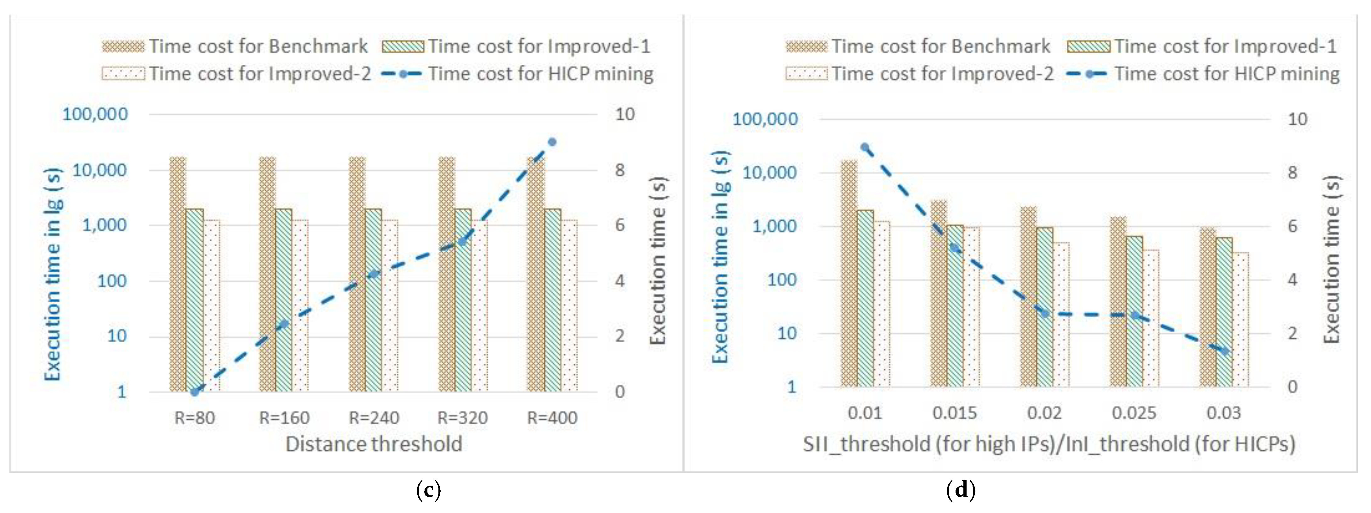
• Effect of distance threshold on efficiency

The histograms of Figure 8c show that the high IP mining algorithms held their time costs at 8.472, 6.594, and 6.173 s regardless of variation in R. In sharp contrast, when the distance threshold R rose within [80, 400], the time cost of the HICP mining algorithm (blue dashed line) exponentially rose from initial 0.806 s at R = 80 through 17.578 s at R = 160 to 31,499.259 s at R = 400. These results reveal that the HICP mining algorithm ran slower by 1~4 orders of magnitude than the high IP mining algorithms when R varied within [80, 400].

• Effect of SII_threshold/InI_threshold on efficiency

The histograms of Figure 8d show that the time costs of high IP mining algorithms slightly fluctuated around 6.9066, 5.9554, and 5.5314 s with the rise of SII_threshold within [0.01, 0.03]. On the contrary, when InI_threshold rose within [0.01, 0.03], the time cost of the HICP mining algorithm (blue dashed line) exponentially fell from initial 31,499.259 s at InI_threshold = 0.01 through 23.574 s at InI_threshold = 0.02 to 4.855 s at InI_threshold = 0.03. This shows that most HICPs were concentrated within a range of 0 $\le$ InI_threshold $\le$ 0.02, while the high IPs had a wider variety of influence levels.

5.4. Scalability of High IP Mining Algorithms

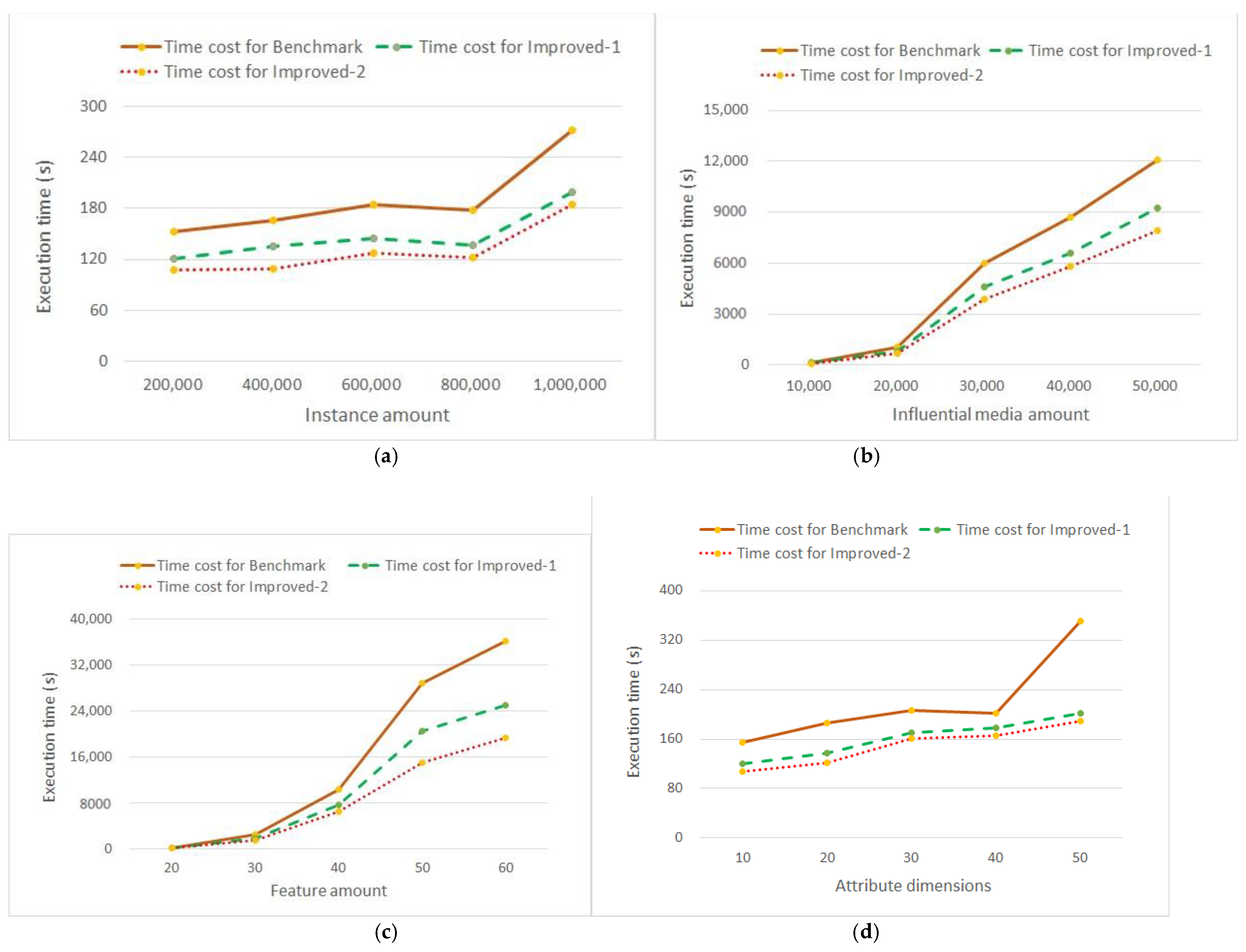
The scalability of high IP mining algorithms were evaluated with variations of four aspects, i.e., instance amount, influential media amount, feature amount, and attribute dimensions, over Syn-2~18 synthetic datasets. The experiments shared a variable as default: SII_threshold = 0.01.

• Effect of instance amount on scalability

The experiment ran on the Syn-2~6 datasets. To evaluate the effect of instance amount on the scalability of the algorithms, we randomly and uniformly distributed 10,000 influential media to the instances of each aforementioned dataset. Figure 9a shows that as the number of instances increased, the time costs of those algorithms did not monotonically increase or decrease but instead varied within a numerical range of [107, 272] s, showing a certain range of random fluctuation. This was because the data synthesizer usually specified a random instance amount for a feature when creating a synthetic dataset, and the instance amounts under a specific feature were different in distinct synthetic datasets. Since high IP mining is based on the proximate relations between instances with distinct features, the occurrence of more instances under the same feature in a dataset causes fewer table instances of IPs and less time costs, or vice versa. Therefore, the increase in the number of instances had no effect on the scalability of the algorithms, unless the distribution of instances changed the relevant factors for mining high IPs. The experimental results showed that compared to Benchmark, Improved-1 and Improved-2 ran 23% and 32% faster, respectively, on average.

• Effect of influential media amount on scalability

We ran experiments on the Syn-2 and Syn-7~10 datasets. Figure 9b shows that with the rise of influential media within a numerical range of [10,000, 50,000], the time costs of the algorithms rose at a quadratic rate. This was because the algorithms mined high influencing patterns on the basis of semantic proximate relations, which were generated as per the directed edges between influential instances. As up to $C_n^2$ edges could be created for n nodes, thus the time costs of the algorithms rose at a quadratic rate as the influential media increased. The experiment showed that compared to Benchmark, Improved-1 and Improved-2 ran 24% and 33% faster, respectively, on average.

• Effect of feature amount on scalability

We ran experiments on the Syn-2 and Syn-11~14 datasets. Figure 9c shows that the time costs of high IP mining algorithms increased cubically when the feature amount rose within a numerical range of [20, 60]. The experiment showed that compared to Benchmark, Improved-1 and Improved-2 ran 27% and 41% faster, respectively, on average.

• Effect of attribute dimensions on scalability

We ran experiments on the Syn-2 and Syn-15~18 datasets. Figure 9d shows that the time costs of the high IP mining algorithms had an up to 69 s difference with the rise of attribute dimensions, that is attribute dimensions had small effects on the scalability of the algorithms. As attribute data were mainly used for calculating influences between instances of distinct features, attribute-related computation used much less time than the discovery of influencing patterns. This fact is conducive to research on the expansion of attribute dimensions in the field of pattern recognition. The experiments showed that compared to Benchmark, Improved-1 and Improved-2 ran 26% and 31% faster, respectively, on average.

6. Discussion and Conclusions

The authors of this study used influential medium flows rather than spatial distance to create semantic proximate relations between instances of distinct features, which overcame the shortage of existing approaches that mine high influence co-location patterns with spatial distance. Accordingly, we cancelled the distance threshold to reduce human interference in the mining process. Experiments verified that our methods are feasible to discover high influencing patterns that cannot be found by HICP mining, and they are also more efficient than HICP mining, whose efficiency is much similar to the classic join-less algorithm [28]. As such, our methods can be considered an effective extension of existing high influence co-location pattern mining approaches, especially for pattern discovery in an influence propagation process.

As this study was focused on realizing high influencing pattern discovery in an influence propagation process by establishing semantic proximity based on influential medium flows between instances and using non-spatial attributes to evaluate influences of influencing pattern, our method does not emphasize efficiency boosts and operates on instances to calculate influences of features via star table instances. In the future, we will try to improve the efficiency of our methods from two promising directions.

One direction is the application of unsupervised clustering technologies. Clustering analysis has the advantages of automatic processing and fast speed, and Huang et al. [50] first discussed the relationship between clustering and spatial co-location pattern; they mainly divided clustering into layer-based clustering (i.e., instances of distinct features are clustered on different layers) and hybrid clustering (i.e., instances of distinct features are clustered on the same layer). Usually, clustering is performed based on instances, but the number of instances is far greater than the number of features in space; therefore, the researchers proposed a clustering idea based on features. Wang and Lei et al. [26,51] followed this idea and defined fuzzy proximity relations on instances before deriving fuzzy proximity relations on features and successfully applying clustering methods, i.e., fuzzy c-medoids clustering, fuzzy hierarchical clustering, and fuzzy density peak clustering, to mine prevalent co-location patterns. Although the clustering methods ran fast, it was difficult and time-consuming to determine the optimal number of clusters and remove outliers. However, the authors of this study required instances to present in a star-shaped structure and needed non-spatial attributes to evaluate influence, that are different from what the traditional clustering methods can meet. There are still many problems to be studied, such as how to deduce the semantic proximity of features from the semantic proximity of instances and how to calculate the similarity and dissimilarity between features based on influence.

Another direction is the use of self-learning methods. In recent years, machine learning technologies have been widely studied and applied. Research on self-encoding learning and attribute coupling analysis [52,53], as well as tensor-based computation and deep attributed network embedding [54,55], has provided many new prospects for high influencing pattern mining research. As our research involves semantic proximity and scalable non-spatial attribute analysis, it will be exciting to apply new technologies here. This article provides a basis for us to explore the interactive relationships between spatial features in attribute and heterogeneous networks.

In other research directions, association rule mining may provide new ideas, as spatial association rule mining is an important extension of association rule mining in traditional transaction databases. Spatial co-location patterns are similar to frequent item sets in transaction databases. However, the spatial co-location rule problem is different from the association rule problem since there is no natural notion of transactions in spatial data sets that are embedded in continuous geographic space. The methods of finding co-location patterns from spatial data mainly include methods based on spatial statistics and data mining. With the increasing number of spatial instances and features, the number of candidate patterns to be tested by statistical method has exponentially increased. The method based on data mining is the main spatial co-location pattern mining method because of its computational efficiency. We have noticed that GA-Apriori and PSO-Apriori [56] algorithms have good results in association rule mining because the item sets in association rule mining do not have spatial coordinates or attributes, there is no need to calculate the relations between them except to identify whether they are in the same transaction, and the item sets do not belong to distinct categories. The problems faced by association rules and spatial co-location pattern mining are different, e.g., the genetic algorithm and the particle swarm algorithm adopt the traversal method that the spatial co-location pattern mining tries to reduce as much as possible. However, those algorithms could provide new prospects for our research in the future.

References

- Shekhar, S.; Huang, Y. Discovering Spatial Co-Location Patterns: A Summary of Results. Lect. Notes Comput. Sci. 2001, 2121, 236–256. [Google Scholar] [CrossRef]
- Li, J.; Adilmagambetov, A.; Jabbar, M.S.M.; Zaïane, O.R.; Osornio-Vargas, A.; Wine, O. On discovering co-location patterns in datasets: A case study of pollutants and child cancers. GeoInformatica 2016, 20, 651–692. [Google Scholar] [CrossRef] [Green Version]
- Yu, W. Spatial co-location pattern mining for location-based services in road networks. Expert Syst. Appl. 2016, 46, 324–335. [Google Scholar] [CrossRef]
- Zhang, D.; Guo, Z.; Guo, F.; Dong, Y. An offline map matching algorithm based on shortest paths. Int. J. Geogr. Inf. Sci. 2021, 2, 1–24. [Google Scholar] [CrossRef]
- Wang, Y.; Zeng, D.; Zheng, X.; Wang, F. Propagation of online news: Dynamic patterns. In Proceedings of the 2009 IEEE International Conference on Intelligence and Security Informatics, Richardson, TX, USA, 8–11 June 2009; pp. 257–259. [Google Scholar] [CrossRef]
- Chen, Z. Epidemic Thresholds in Networks: Impact of Heterogeneous Infection Rates and Recovery Rates. In Proceedings of the 2018 IEEE International Conference on Communications (ICC), Kansas City, MO, USA, 20–24 May 2018; pp. 1–6. [Google Scholar] [CrossRef]
- Jiang, C.; Zhang, Y.; Wang, H.; Zhou, Y.; Zou, Y. Study on Coupled Social Network Public Opinion Communication Based on Improved SEIR. In Proceedings of the 2020 IEEE International Conference on Parallel & Distributed Processing with Applications, Big Data & Cloud Computing, Sustainable Computing & Communications, Social Computing & Networking (ISPA/BDCloud/SocialCom/SustainCom), Exeter, UK, 17–19 December 2020; pp. 1495–1500. [Google Scholar] [CrossRef]
- Michael, F.G. The validity and usefulness of laws in geographic information science and geography. Ann. Assoc. Am. Geogr. 2004, 94, 300–303. [Google Scholar] [CrossRef] [Green Version]
- Tobler, W. On the First Law of Geography: A Reply. Ann. Assoc. Am. Geogr. 2004, 94, 304–310. [Google Scholar] [CrossRef]
- Yu, W. Identifying and Analyzing the Prevalent Regions of a Co-Location Pattern Using Polygons Clustering Approach. ISPRS Int. J. Geo-Infor. 2017, 6, 259. [Google Scholar] [CrossRef] [Green Version]
- Li, X.; Cao, C.; Chang, C. The first law of geography and spatio-temporal proximity. Chin. J. Nat. 2007, 29, 69–71. Available online: https://www.nature.shu.edu.cn/CN/Y2007/V29/I2/69 (accessed on 14 October 2021).
- Brockmann, D.; Hufnagel, L.; Geisel, T. The scaling laws of human travel. Nature 2006, 439, 462–465. [Google Scholar] [CrossRef]
- Barua, S.; Sander, J. Mining Statistically Significant Co-Location and Segregation Patterns. IEEE Trans. Knowl. Data Eng. 2013, 26, 1185–1199. [Google Scholar] [CrossRef]
- Duan, J.; Wang, L.; Hu, X. The effect of spatial autocorrelation on spatial co-location pattern mining. In Proceedings of the 2017 International Conference on Computer, Information and Telecommunication Systems (CITS), Dalian, China, 21–23 July 2017; pp. 210–214. [Google Scholar] [CrossRef]
- Wang, L.; Bao, X.; Zhou, L.; Chen, H. Maximal Sub-Prevalent Co-Location Patterns and Efficient Mining Algorithms. In Proceedings of the International Conference on Web Information Systems Engineering, Puschino, Russia, 7–11 October 2017; Bouguettaya, A., Gao, Y., Klimenko, A., Eds.; Springer: Cham, Switzerland, 2017; pp. 199–214. [Google Scholar] [CrossRef]
- Wang, L.; Bao, X.; Zhou, L.; Chen, H. Mining maximal sub-prevalent co-location patterns. World Wide Web 2019, 22, 1971–1997. [Google Scholar] [CrossRef]
- Huang, Y.; Shekhar, S.; Xiong, H. Discovering Colocation Patterns from Spatial Datasets: A General Approach. IEEE Trans. Knowl. Data Eng. 2004, 16, 1472–1485. [Google Scholar] [CrossRef] [Green Version]
- Yoo, J.S.; Shekhar, S.; Smith, J.; Kumquat, J.P. A partial join approach for mining co-location patterns. In Proceedings of the 12th annual ACM international workshop on Geographic information systems—GIS ’04, Washington, DC, USA, 12–13 November 2004; pp. 241–249. [Google Scholar] [CrossRef]
- Yoo, J.S.; Shekhar, S.; Celik, M. A Join-Less Approach for Co-Location Pattern Mining: A Summary of Results. In Proceedings of the Fifth IEEE International Conference on Data Mining (ICDM’05), Houston, TX, USA, 27–30 November 2006; p. 4. [Google Scholar] [CrossRef]
- Wang, L.; Bao, Y.; Lu, J.; Yip, J. A new join-less approach for co-location pattern mining. In Proceedings of the 2008 8th IEEE International Conference on Computer and Information Technology, Sydney, NSW, Australia, 8–11 July 2008; pp. 197–202. [Google Scholar] [CrossRef]
- Wang, L.; Bao, Y.; Lu, Z. Efficient discovery of spatial co-location patterns using the iCPI-tree. Open Inf. Syst. J. 2009, 3, 69–80. [Google Scholar] [CrossRef] [Green Version]
- Yao, X.; Peng, L.; Yang, L.; Chi, T. A fast space-saving algorithm for maximal co-location pattern mining. Expert Syst. Appl. 2016, 63, 310–323. [Google Scholar] [CrossRef]
- Bao, X.; Wang, L. A clique-based approach for co-location pattern mining. Inf. Sci. 2019, 490, 244–264. [Google Scholar] [CrossRef]
- Tran, V.; Wang, L.; Chen, H.; Xiao, Q. MCHT: A maximal clique and hash table-based maximal prevalent co-location pattern mining algorithm. Expert Syst. Appl. 2021, 175, 114830. [Google Scholar] [CrossRef]
- Wang, L.; Jiang, W.; Chen, H.; Fang, Y. Efficiently Mining High Utility Co-Location Patterns from Spatial Data Sets with In-Stance-Specific Utilities. In Proceedings of the International Conference on Database Systems for Advanced Applications (DASFAA ’17), Taipei, Taiwan, 11–14 April 2021; Candan, S., Chen, L., Pedersen, T., Eds.; Springer: Cham, Switzerland, 2017; pp. 458–474. [Google Scholar] [CrossRef]
- Wang, X.; Lei, L.; Wang, L.; Yang, P.; Chen, H. Spatial Co-location Pattern Discovery Incorporating Fuzzy Theory. In IEEE Transactions on Fuzzy Systems; IEEE: Piscataway, NJ, USA, 2021; p. 1. [Google Scholar] [CrossRef]
- Chen, L. Spatial High Impact Co-Location Pattern Mining. Master’s Thesis, Yunnan University, Kunming, China, 2017. Available online: http://113.55.8.26/search/article?id=15501 (accessed on 14 October 2021).
- Fang, D.; Wang, L.; Yang, P.; Chen, L. Mining high influence co-location patterns from instances with attributes. Evol. Intell. 2019, 13, 197–210. [Google Scholar] [CrossRef]
- Lei, L.; Wang, L.; Zeng, Y.; Zeng, L. Discovering High Influence Co-Location Patterns from Spatial Datasets. In Proceedings of the 2019 IEEE International Conference on Big Knowledge (ICBK ’19), Beijing, China, 10–11 November 2019; pp. 137–144. [Google Scholar] [CrossRef]
- Ma, D.; Chen, H.; Wang, L.; Xiao, Q. Dominant feature mining of spatial sub-prevalent co-location patterns. J. Comput. Appl. 2019, 40, 465–472. [Google Scholar] [CrossRef]
- Shang, Y.; Fan, X.; Yu, H. A node influence measurement algorithm based on characteristics of users and propagation. Comput. Eng. Sci. 2015, 37, 2105–2111. Available online: http://en.cnki.com.cn/Article_en/CJFDTotal-JSJK201511017.htm (accessed on 14 October 2021).
- Li, W.; Li, C.; Geng, Y. APS: Attribute-aware privacy-preserving scheme in location-based services. Inf. Sci. 2020, 527, 460–476. [Google Scholar] [CrossRef]
- Citraro, S.; Rossetti, G. Eva: Attribute-aware Network Segmentation. In Complex Networks and Their Applications VIII, Proceedings of the International Conference on Complex Networks and Their Applications VIII, Lisbon, Portugal, on 10–12 December 2019; Cherifi, H., Gaito, S., Mendes, J.F., Moro, E., Rocha, L.M., Eds.; Springer: Cham, Switzerland, 2020; Volume 881, pp. 141–151. [Google Scholar] [CrossRef] [Green Version]
- Subbian, K.; Aggarwal, C.; Srivastava, J. Content-centric flow mining for influence analysis in social streams. In Proceedings of the 22nd ACM International Conference on Conference on Information & Knowledge Management-CIKM ’13, San Francisco, CA, USA, 27 October–1 November 2013; ACM Press: New York, NY, USA, 2013; pp. 841–846. [Google Scholar] [CrossRef] [Green Version]
- Yoo, J.S.; Shekhar, S.; Kim, S.; Celik, M. Discovery of Co-evolving Spatial Event Sets. In 2006 SIAM International Conference on Data Mining; Society for Industrial & Applied Mathematics (SIAM): University City, PA, USA, 2006; pp. 306–315. [Google Scholar] [CrossRef] [Green Version]
- Celik, M.; Shekhar, S.; Rogers, J.P.; Shine, J.A.; Yoo, J.S. Mixed-drove Spatio-temporal Co-occurence Pattern Mining: A Summary of Results. In Proceedings of the Sixth International Conference on Data Mining (ICDM’06), Hong Kong, China, 18–22 December 2006; pp. 119–128. [Google Scholar] [CrossRef]
- Celik, M.; Shekhar, S.; Rogers, J.P.; Shine, J.A. Sustained Emerging Spatio-Temporal Co-occurrence Pattern Mining: A Summary of Results. In Proceedings of the 2006 18th IEEE International Conference on Tools with Artificial Intelligence (ICTAI’06), Arlington, VA, USA, 13–15 November 2006; pp. 106–115. [Google Scholar] [CrossRef] [Green Version]
- Celik, M.; Shekhar, S.; Rogers, J.P.; Shine, J.A.; Kang, J.M. Mining at Most Top-K% Mixed-drove Spatio-temporal Co-occurrence Patterns: A Summary of Results. In Proceedings of the 2007 IEEE 23rd International Conference on Data Engineering Workshop, Istanbul, Turkey, 17–20 April 2007; pp. 565–574. [Google Scholar] [CrossRef]
- Qian, F.; He, Q.; He, J. Mining Spread Patterns of Spatio-temporal Co-occurrences over Zones. In Lecture Notes in Computer Science; Gabler: Seoul, Korea, 2009; pp. 677–692. [Google Scholar] [CrossRef]
- Celik, M. Discovering partial spatio-temporal co-occurrence patterns. In Proceedings of the 2011 IEEE International Conference on Spatial Data Mining and Geographical Knowledge Services, Fuzhou, China, 29 June–1 July 2011; pp. 116–120. [Google Scholar] [CrossRef]
- Qian, F.; Yin, L.; He, Q.; He, J. Mining spatio-temporal co-location patterns with weighted sliding window. In Proceedings of the 2009 IEEE International Conference on Intelligent Computing and Intelligent Systems, Shanghai, China, 20–22 November 2009; Volume 3, pp. 181–185. [Google Scholar] [CrossRef]
- Huang, Y.; Zhang, L.; Zhang, P. A Framework for Mining Sequential Patterns from Spatio-Temporal Event Data Sets. IEEE Trans. Knowl. Data Eng. 2008, 20, 433–448. [Google Scholar] [CrossRef] [Green Version]
- Hufnagel, L.; Brockmann, D.; Geisel, T. Forecast and control of epidemics in a globalized world. Proc. Natl. Acad. Sci. USA 2004, 101, 15124–15129. [Google Scholar] [CrossRef] [Green Version]
- Chen, L.; Gao, Y.; Fang, Z.; Miao, X.; Jensen, C.S.; Guo, C. Real-time distributed co-movement pattern detection on streaming trajectories. In VLDB Endowment; VLDB Endowment: Los Angeles, CA, USA, 2019; Volume 12, pp. 1208–1220. [Google Scholar] [CrossRef] [Green Version]
- Hu, X.; Wang, G.; Duan, J. Mining Maximal Dynamic Spatial Co-Location Patterns. IEEE Trans. Neural Netw. Learn. Syst. 2021, 32, 1026–1036. [Google Scholar] [CrossRef] [Green Version]
- Moosavi, S.; Samavatian, M.H.; Nandi, A.; Parthasarathy, S.; Ramnath, R. Short and Long-Term Pattern Discovery over Large-Scale Geo-Spatio-Temporal Data. In Proceedings of the 25th ACM SIGKDD International Conference on Knowledge Discovery and Data Mining (KDD ’19), Anchorage, AK, USA, 4–8 August 2019; Assoc Comp Machinery: New York, NY, USA, 2019; pp. 2905–2913. [Google Scholar] [CrossRef] [Green Version]
- Shekhar, S.; Jiang, Z.; Ali, R.Y.; Eftelioglu, E.; Tang, X.; Gunturi, V.M.V.; Zhou, X. Spatio-temporal data mining: A computational perspective. ISPRS Int. J. Geo-Inf. 2015, 4, 2306–2338. [Google Scholar] [CrossRef]
- Feng, K.; Cong, G.; Jensen, C.S.; Guo, T. Finding attribute-aware similar regions for data analysis. In Proceedings of the VLDB Endowment; VLDB Endowment: Los Angeles, CA, USA, 2019; Volume 12, pp. 1414–1426. [Google Scholar] [CrossRef]
- Saaty, T.L. Priority setting in complex problems. IEEE Trans. Eng. Manag. 1983, 30, 140–155. [Google Scholar] [CrossRef]
- Huang, Y.; Zhang, P.; Zhang, C. On the Relationships between Clustering and Spatial Co-Location Pattern Mining. Int. J. Artif. Intell. Tools 2008, 17, 55–70. [Google Scholar] [CrossRef] [Green Version]
- Lei, L.; Wang, L.; Wang, X. Mining Spatial Co-Location Patterns by the Fuzzy Technology. In Proceedings of the 2019 IEEE International Conference on Big Knowledge (ICBK), Beijing, China, 10–11 November 2019; pp. 129–136. [Google Scholar] [CrossRef]
- Li, Z.; Wang, X.; Li, J.; Zhang, Q. Deep attributed network representation learning of complex coupling and interaction. Knowl.-Based Syst. 2021, 212, 106618. [Google Scholar] [CrossRef]
- Wang, C.; Dong, X.; Zhou, F.; Cao, L.; Chi, C.-H. Coupled Attribute Similarity Learning on Categorical Data. IEEE Trans. Neural Netw. Learn. Syst. 2014, 26, 781–797. [Google Scholar] [CrossRef]
- He, L.; Lu, C.-T.; Chen, Y.; Zhang, J.; Shen, L.; Yu, P.S.; Wang, F. A Self-Organizing Tensor Architecture for Multi-view Clustering. In Proceedings of the 2018 IEEE International Conference on Data Mining (ICDM), Singapore, 17–20 November 2018; pp. 1007–1012. [Google Scholar] [CrossRef] [Green Version]
- Hong, R.; He, Y.; Wu, L.; Ge, Y.; Wu, X. Deep Attributed Network Embedding by Preserving Structure and Attribute Information. IEEE Trans. Syst. Man. Cybern. Syst. 2021, 51, 1434–1445. [Google Scholar] [CrossRef]
- Djenouri, Y.; Comuzzi, M. Combining Apriori heuristic and bio-inspired algorithms for solving the frequent itemsets mining problem. Inf. Sci. 2017, 420, 1–15. [Google Scholar] [CrossRef]
Figure 1.
Demonstration of an influence propagation process within a specific period. (a) Instance B.1 has cumulative influence on instance A.2 until moment ti, reflected by attribute vectors of the influencing instance and the directed edge; (b) influential media flows moving between instances of distinct features within a time span (e.g., T1 = (t0, t1]) are depicted at last moment (e.g., t1); (c) influence propagation digraphs at different moments.
Figure 2.
An example of an influence propagation digraph at a specific moment.
Figure 3.
A proposed framework for mining high IPs.
Figure 4.
An illustration that shows the star neighbor instance set, candidate patterns, and three-layer hashmap structure obtained from Figure 2, where the central features of candidate patterns are marked with an * superscript to improve readability.
Figure 5.
An example of decomposition of the unqualified patterns by a central feature to sub candidate patterns at a smaller size, based on Figure 2, where the central features of candidate patterns are marked with an * superscript to improve readability.
Figure 6.
(a) A distribution map for the studied POIs (cities) in mainland China; (b) a UI that shows inter-city human migration trends at the Baidu Map Smart Eye site.
Figure 7.
(a) Effect of distance threshold on pattern amount on the Real-1 dataset; (b) effect of SIIthreshold/InIthreshold on pattern amount on the Real-1 dataset.
Figure 8.
(a) Effect of distance threshold on efficiency (over the Real-1 dataset); (b) effect of SIIthreshold/InIthreshold on efficiency (over the Real-1 dataset); (c) effect of distance threshold on efficiency (over the Syn-1 dataset); (d) effect of SIIthreshold/InIthreshold on efficiency (over the Syn-1 dataset).
Figure 9.
Comparison of the scalability of high IP mining algorithms with variations of: (a) instance amount, (b) influential media amount, (c) feature amount, and (d) attribute dimensions.