
Integration Development of Urban Agglomeration in Central Liaoning, China, by Trajectory Gravity Model

Transportation Engineering Department, Shenyang Jianzhu University, Shenyang 110000, China
*
Author to whom correspondence should be addressed.
ISPRS Int. J. Geo-Inf. 2021, 10(10), 698; https://0-doi-org.brum.beds.ac.uk/10.3390/ijgi10100698
Submission received: 2 August 2021
/
Revised: 1 October 2021
/
Accepted: 4 October 2021
/
Published: 14 October 2021
(This article belongs to the Special Issue Geo-Information Science in Planning and Development of Smart Cities)
Abstract
:Integration development of urban agglomeration is important for regional economic research and management. In this paper, a method was proposed to study the integration development of urban agglomeration by trajectory gravity model. It can analyze the gravitational strength of the core city to other cities and characterize the spatial trajectory of its gravitational direction, expansion, etc. quantitatively. The main idea is to do the fitting analysis between the urban axes and the gravitational lines. The correlation coefficients retrieved from the fitting analysis can reflect the correlation of two indices. For the different cities in the same year, a higher value means a stronger relationship. There is a clear gravitational force between the cities when the value above 0.75. For the most cities in different years, the gravitational force between the core city with itself is increasing by years. At the same time, the direction of growth of the urban axes tends to increase in the direction of the gravitational force between cities. There is a clear tendency for the trajectories of the cities to move closer together. The proposed model was applied to the integration development of China Liaoning central urban agglomeration from 2008 to 2016. The results show that cities are constantly attracted to each other through urban gravity.
1. Introduction
Urban agglomeration are clusters of cities that have the characteristics of agglomeration, innovation, and outward orientation in the context of increasing urbanization [1]. Urban agglomerations affect each other in terms of economic linkages, industrial labor division and cooperation, transport, social life, urban planning, and infrastructure development, and become an inevitable trend in urban development [2]. The development of China’s urban strategy is centered on mega-cities, driving neighboring cities to develop together. Central Liaoning urban agglomeration is an important gateway to the opening of northeast of China, and the study of its integration development is of great significance to the construction of “One Belt, One Road”, the promotion of new types of urbanization, and the overall revitalization of the northeast of China.
The drivers of urban development have been the focus of regional development research. Existing studies of drivers are usually based on data from cities’ level of development, where one of the most important factors is the economy. Lin et al. pointed out that Per capita GDP is the basic driving force of urbanization and the marginal utility of GDP growth tends to decrease with the expansion of urbanization [3]. Xu et al. used regression models to demonstrate the influence of human, climatic and physical drivers on land use change within the context of rapid urbanization in China [4]. Although data are a good representation of development, they lack a description of the interrelationships between different cities. The urban gravity model derives from the law of universal gravitational and is one of the main methods for studying the integration development of urban agglomeration [5]. However, current research on integrated development of urban agglomeration based on gravity model focuses more on the spatial description of gravity trajectories. For example, Zhang et al. used population migration to construct a gravity model and analyzed the effect of gravity strength on the relationship between cities [6]; Chen et al. introduced fractal theory into the urban gravity model to improve the accuracy of gravitational strength description [7]; the relationship between gravitational strength and urban structure was discussed by Burger et al. [8]. Some of the above studies have only considered the structural aspect of the city itself and do not consider the impacts of other cities on themselves. Some have considered the interaction of information between different cities without considering one of the more important spatial information between cities, the distance. Based on spatial distance as an important factor, the urban gravity model takes some indicators that have been shown to be associated with urban development, such as economic, demographic, and energy, as gross size and describes the gravity strength between cities by analyzing the variation of gross sizes and spatial distance. Trajectory and intensity are two important properties of gravity, and trajectory description is another key of addressing a complete representation of gravity.
The evolution of urban axis reflects the trajectory of urban development, and can provide one of the main bases for describing the gravity trajectory of urban agglomeration [9]. In general, some researchers use the skeleton lines of urban built-up areas as the urban axis. The method of extracting the skeleton lines in the urban built-up areas is divided into two parts: extracting the built-up areas and extracting the skeleton lines. Night-time lighting images and Landsat images are the main data sources for extracting built-up areas [10,11]. The extraction of skeleton lines is mainly performed by parallel line cutting midpoint linking method, Delaunay triangulation method, Voronoi plot method, and curvature calculation method [12]. Delaunay triangulation method uses discrete points on polygon boundaries to build triangles, and skeleton lines are constructed by connecting feature points on triangles. Delaunay triangulation method is the more commonly used for trend analysis of polygons, and can provide the reference for the extraction of gravity trajectory.
This paper aims to propose a method based on the trajectory gravity model for the integration development of urban agglomeration and applied to China Central Liaoning urban agglomeration. The method cannot describe only the gravity strength between cities, but also the gravity trajectory, which provides a deeper understanding of the development of urban integration.
Firstly, we pre-process the night-time lighting data and Landsat data by radiation correction, fusion, geometry correction, etc.
Secondly, the normalized differentiated built-up area index is constructed by grayscale values of night-time lighting data and impervious surface indices of Landsat data. The urban built-up areas are extracted by Statistical Comparison Method. Multisource data can take advantage of different data, and it is of great research significance to study a method of built-up area extraction that integrates night-time lighting data and Landsat data.
Thirdly, gravity strength between cities is calculated by urban gravity models, which can quantitatively describe the interaction.
Fourthly, the Delaunay triangular networks of built-up area polygons are constructed, and the skeleton lines are extracted as urban axis by the triangular feature point analysis method.
Finally, we analyze the development of urban integration by the changes in gravity intensity and urban axis. In addition, the proposed method is compared with other methods, and its main advantages and disadvantages are summarized.
2. Study Areas and Data
2.1. Study Areas
The Chinese government issued three regions and ten urban agglomerations as the key regions during the 12th Five-Year Plan in October 2012. The three regions include Beijing-Tianjin-Hebei region, Yangtze River Delta region, and Pearl River Delta region. Central Liaoning is included in ten urban agglomerations [13].
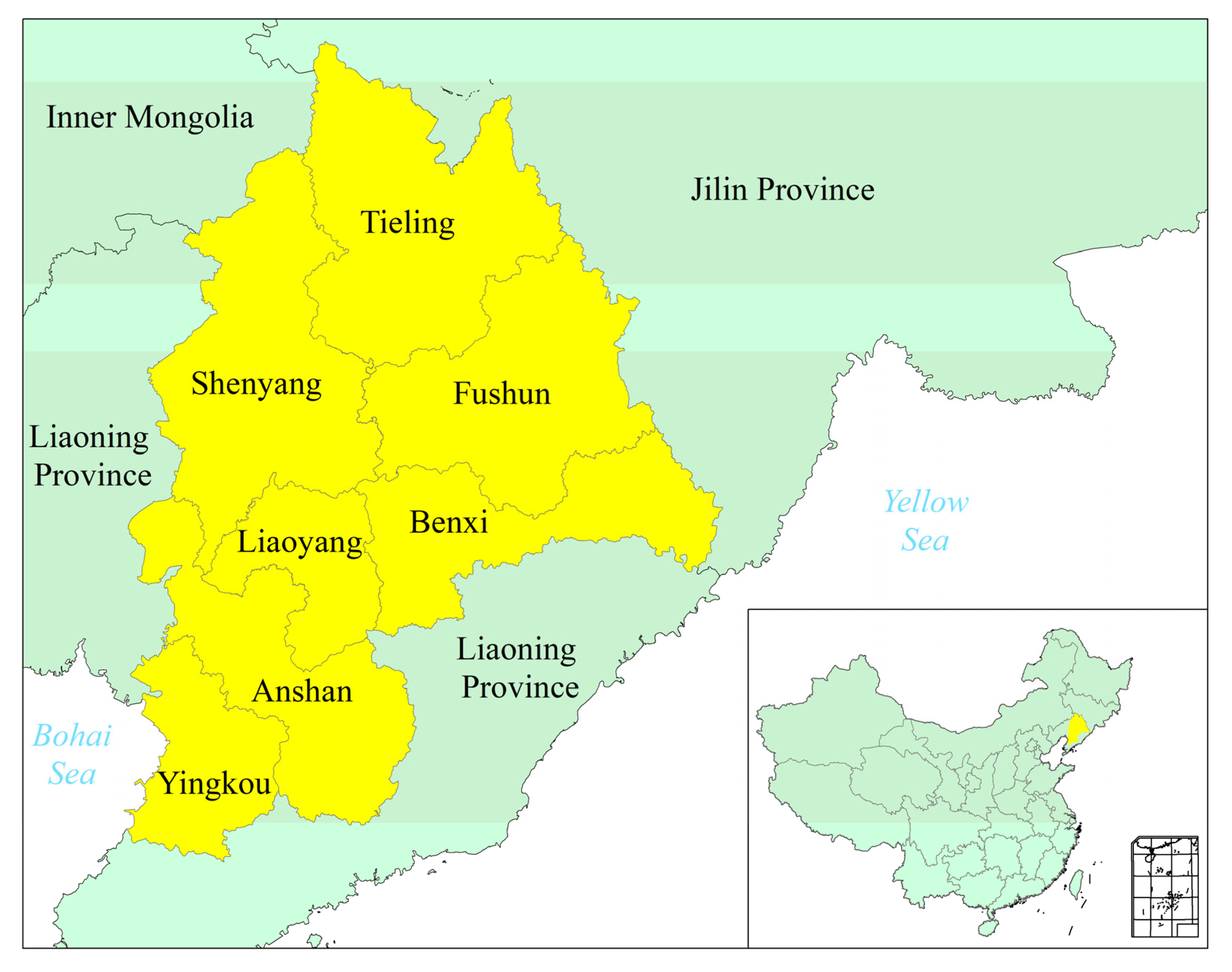
Liaoning is a developing province located in northeastern China. China Central Liaoning urban agglomeration is an important part of the Northeast Economic Zone and Bo Sea Metropolitan Area, which includes Shenyang, Anshan, Fushun, Benxi, Yingkou, Liaoyang, and Tieling. Shenyang is the core city. The location is shown in Figure 1. Although it has a low level of development and is still at the stage of rapid development and spatial agglomeration, there are many policies proposed for the sake of regional synergy. Shenyang proposes the spatial development planning strategy of “Expansion towards South, North, and West, Eastward Optimization”. Fushun expands westward in order to realize the co-urbanization of Shenyang and Fushun. The overall spatial function between Anshan, Benxi, and Liaoyang is further optimized. Shiqiaozi Development Zone in Benxi develops westward, close to Hunnan District of Shenyang. Tieling is actively building the Shenyang Railway Industrial Corridor for creating Tieling New Town and Xintaizi High-tech Industrial Zone, which is linked to the North District of Shenyang.
2.2. Data
2.2.1. Landsat Data
This paper used Landsat TM/ETM+ images published by NASA to extract impervious surfaces in cities [14,15]. Impervious surface is an important indicator of urban built-up areas and the degree of expansion directly reflects the expansion of urban built-up areas. Landsat TM data consist of seven bands with a spatial resolution of 30 m. Landsat ETM+ data consist of nine bands with a spatial resolution of 30 m and one band has a resolution of 15 m. Landsat images can collect the land cover data and have a high spatial resolution. In general, some researchers extract built-up areas in Landsat images by constructing impervious surface indexes, and the results are more effective in describing the details [16]. However, the spectra of Landsat data pixels have a certain complexity, which not only make the extraction more difficult, but also result in a higher fragmentation. It is necessary to process some small spots to obtain a complete built-up area [17].
2.2.2. Night-Time Lighting Data
Night-time lighting images can describe the spatial distribution of urban economy and population, the main methods include statistical analysis method, clustering analysis method, spatial constraint method, extraction results have the advantage of high integrity [18,19,20]. However, there is a light spillover effect in the night-time light images, which makes the extraction results have a high false detection rate.
DMSP/OLS data are from the National Oceanic and Atmospheric Administration (NOAA) of the United States. So far, NOAA has released three types of nighttime light data: stable light images, radiometric mean light intensity images, and nonradiometric mean light intensity images. Currently, the widely used one is the stable light image. This image includes town lights and persistent light sources from other locations, and the raster removes the effects of transient or incidental noise such as moonlight clouds, light fires, and oil and gas combustion. Its brightness values range from 0 to 63 and its spatial resolution is 1 km. We select the data from F16 and F18 sensors, which the years of data are 2008 and 2012.
NPP/VIIRS data are also from the National Oceanic and Atmospheric Administration (NOAA) of the United States. It has a higher resolution of 430 m from 2013 to 2016 [21] and shows more details. As DMSP/OLS data ceased to be received in 2013, NPP/VIIRS data for August 2016 are selected.
2.2.3. Vector Map and Statistical Data
The vector map for provincial, municipal, and county administrative divisions in China are from the National Center for Basic Geographic Information. Download Website: www.webmap.cn (accessed on 4 October 2021).; Scale: 1:4 million; Coordinate System: WGS-84.
The data of built-up areas for each year are taken from the statistical yearbooks in the China Economic and Social Development Database. Download Website: https://data.cnki.net (accessed on 4 October 2021).
3. Methods
3.1. Data Pre-Processing
3.1.1. Landsat Data Pre-Processing
Firstly, the Landsat images were processed by band fusion and multitemporal image alignment was performed using a polynomial algorithm. Secondly, the linear stretching algorithm was used to adjust the grayscale values of the data from 0 to 255. Finally, images were cropped using administrative division vector data to obtain interest data.
3.1.2. DMSP/OLS Data Pre-Processing
Since the 2008 and 2012 DMSP/OLS data are from different sensors, there are oversaturation and discontinuity in the multitemporal data. In order to improve the continuity and stability, the relative radiation correction method based on quadratic regression model [22] was employed in this paper. The quadratic regression model is shown in (1):
where is the relative radiation-corrected gray value, DN is the original image grayscale value, and a, b and c are the correction factors. DMSP/OLS data for 1999 from F12 Sensor were selected as the reference data. The calibrated DNSP/OLS data were re-projected as Asia Lambert Conformal Conic and set to the sampling spatial resolution of 500 m.
3.1.3. NPP/VIIRS Data Pre-Processing
The DMSP/OLS images and the NPP/VIIRS images have different spatial resolutions and range of brightness values. In order to ensure time series consistency and comparability between DMSP/OLS data and NPP/VIIRS data, relative radiation correction of NPP/VIIRS data was performed by DMSP/OLS data as reference data.
Firstly, we used DMSP/OLS data and NPP/VIIRS data from the same year, 2012, to do the regression analysis. From the result of the analysis, we defined the formula and the coefficients. The regression Equation is shown in (2):
where is the corrected gray value and is the original grayscale value of the VIIRS/NPP data.
Secondly, we used the equation to adjust the 2016 NPP/VIIRS to make the image the same brightness values with DMSP/OLS data from 0 to 63.
Finally, the calibrated NPP/VIIRS data were re-projected as Asia Lambert Conformal Conic and set to the sampling spatial resolution of 500 m.
3.2. Urban Built-Up Areas Extraction
Urban built-up area extraction is the first step in conducting the analysis. The main purpose of this step is to extract the urban built-up areas and depict them according to their location. The obtained urban built-up areas also provide data for subsequent processing. Based on the obtained results, we extracted the gray value information and area values. It also provides the basic data source for obtaining the shortest distance between the built-up areas of two cities.
3.2.1. Normalized Differential Built-Up Area Index Construction
Both the night-time lighting image gray values and the Landsat image impervious surface index are proportional to the probability that the pixel belongs to the built-up area [23]. Since built-up areas are the result of the combined interaction of people and land, the night-time lighting images only reflect the spatial distribution patterns of the economy and population, and the Landsat data only provide the objective description of the land surface coverage. To improve the incompleteness of built-up areas extracted by the single data source, the normalized difference built-up area index (NDUBI) was proposed in this paper. The normalized difference impervious surface index (NDISI) of Landsat image was used to form an impervious surface image. The NDISI index formula is shown in (3):
where the MNDWI index formula is shown in (4):
where NIR is the near-infrared value, MIR is the mid-infrared value, and TIR is the thermal infrared value. MNDWI is the corrected normalized water body index and GREEN is the green value. NDUBI takes the sum of the gray values of the night-time lighting image and the impervious surface image as the denominator, its difference as the numerator. NDUBI index formula is shown in (5):
where NTL is the night-time lighting image gray value. The above equation is the empirical formula imitating Equation (3), which fuses multisource data information in the form of difference ratio.
3.2.2. Urban Built-Up Areas Extraction Based on Statistical Comparison Method
The statistical comparison method determines the optimal segmentation threshold for NDUBI images by comparing the similarity between the built-up extraction area and the official statistical built-up area [18,24]. Firstly, the official statistical data of the study area were collected. Secondly, the initial segmentation threshold to separate the NDUBI image was set to 0. The temporary segmentation threshold was increasing from the initial one gradually. The temporary built-up area was the sum of the pixels whose brightness values were larger than the threshold. Then, the temporary segmentation threshold stoped increasing when the absolute value of the difference between the area of the temporary built-up and the area of statistics was lowest. Finally, the temporary segmentation threshold at that moment was defined as the optimal segmentation threshold. We used the optimal threshold to separate the image into two groups, the built-up area and nonurban built-up area.
3.3. Urban Axis Extraction by Delaunay Triangular Network
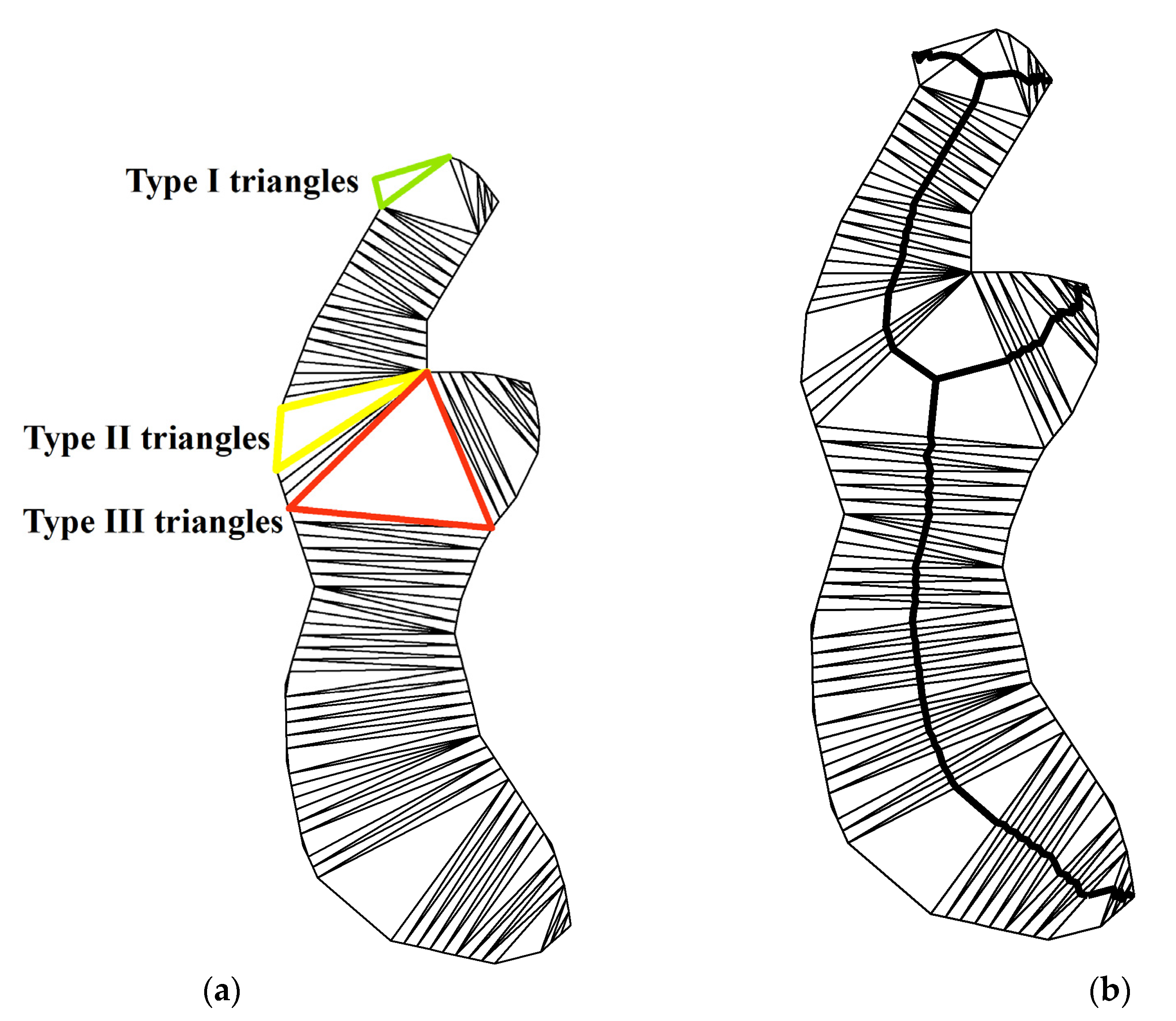
The urban axis is the directional line that describes the spatial expansion abstractly and functional transfer of the city, and it can express the urban evolutionary direction objectively and quantitatively. The contours of urban built-up areas serve as the spatial projection of the urbanization, and their skeleton lines are the objective representation of the urban spatial axis. The main purpose of getting the city axes is to simplify the faces into lines and to show more clearly the direction of urban expansion. Firstly, the Delaunay triangulation network was constructed by equidistant points along the contour line of the built-up area. Secondly, we constructed the initial skeleton lines by the network. The triangles of Delaunay triangulation network were classified into three types: type I, II, III, as shown in Figure 2a. Type I triangles are connected to only one adjacent triangle and take its vertex as the endpoint of the skeleton line segment; Type II triangles have common sides with two adjacent triangles and take the midpoint of the two common sides as the point of the skeleton line segment; Type III triangles have common sides with three adjacent triangles and connect the gravity of the triangle with the midpoint of the three sides of the other triangles to form three skeleton lines. The points from the three types of triangles were connected sequentially to form the initial skeleton line of the built-up area contour. Finally, trim the initial skeleton line. The shorter branches of the skeleton line were eliminated, and the main branches were retained to obtain the final skeleton line of the built-up area, which serves as the urban axis. This is illustrated in Figure 2b.
3.4. Principal Component Analysis on Gross Sizes of Cities
Urban gravity requires a value to represent the level of development of the city, reflecting the social, economic, and other aspects of the indicators. Therefore, we need to make a comprehensive consideration of most aspects of the cities and get a combined result as the gross size. Faced with a variety of urban indicators, we have chosen several mentioned in the paper. In addition, we chose a method that is widely used nowadays, principal component analysis (PCA), in order to integrate multiple parameters effectively and reduce the correlation of parameters.
The drivers of urban development cover various aspects. Under the premise of integrated urban and rural development, the coordinated development of urban and rural areas highlights the function and value of the primary industry in the social economy [25]. Liaoning is also a long-standing industrial province, and the industrial economy of the secondary industry has been an important factor in promoting the development of cities. In today’s information exchange and smart city development, the tertiary industry created by trade flow and information interchange has also made positive contributions to urban development. In this paper, the urban built-up area was extracted as the key factor that could visually reflect the urban construction. From this result, we obtained relevant information, such as area, gray value information, etc., combined with urban infrastructure, population, transportation, and other elements that are closely related to urban development. With the above-mentioned information, we constituted the basic elements used in PCA. So, the parameters in this paper included sum of gray values, mean of gray values, built-up area, added value of primary sector, added value of secondary sector, added value of tertiary sector, population, number of streetlights and urban road area. Among them, the values of primary, secondary, and tertiary industries represented different aspects of urban development, the sum and average of grayscale values and built-up area values represented the experimental extraction results, and population, number of streetlights and road area reflected population, urban infrastructure, and transportation, respectively. All data are from the Chinese Statistical Yearbook for each year except for the sum and mean of gray values.
The principle of principal component extraction is to extract principal components with an eigenvalue greater than 1. The eigenvalue is an indicator of the magnitude of the principal component’s impact. If the eigenvalue is less than 1, it means that the principal component is not as strongly interpreted as an original variable, eigenvalues greater than 1 are used as inclusion criteria.
The main process of PCA is as follows. Firstly, the data in the component matrix was used to calculate the feature vectors of each principal component. We can obtain the variance of each principal component, like . A larger variance indicates more information is covered. Secondly, the feature vectors were multiplied with the standardized values of the parameters. The equation is shown in (6):
where , , …… are the eigenvectors corresponding to the eigenvalues of the covariance array, , , ……, are the normalized values of the original variables. is the final value of the principal component and is the number of the principal component. p is the number of the parameters. Then, the results summed to get the numbers of each principal component. The equation is shown in (7):
Finally, the feature values of each principal component were used as weights to calculate the weighted average, and the principal component composite model values were obtained to represent the gross sizes of cities. The gross size of the city reflects the most aspects of the city as a whole, not only the development within the urban area. As the population used, it includes all population numbers within the urban and rural areas. For the value of growth of primary, secondary, and tertiary industries, both rural and urban areas contribute to its development. Thus, the size only reflects the level of the development of the city in that year, and it is not the exact value and only used in comparison with other cities in the urban agglomeration.
3.5. Urban Gravity Calculation
In the field of urban agglomeration integration, the urban gravity model is one of the classical models reflecting the strength of spatial interactions between cities and is widely used in practice. The urban gravity model is based on Newton’s law of universal gravitational, where the gravitational strength of cities is proportional to the product of their sizes and inversely proportional to the square of their distances. The equation to calculate urban gravity is shown in (8):
where and are the gross sizes of city 1 and city 2, respectively; is the spatial distance between city 1 and city 2; K is the constant coefficient. To avoid the result being too small, K is taken as 1 × 10⁴. In this paper, the distance of the nearest endpoint between two urban axes was taken as the spatial distance.
The urban gravity model captures the strength of linkages and integration trends between cities within urban agglomeration, but it cannot describe the specific processes of integration in space objectively. Based on the principle that the closer the geographic distance is the stronger the geographical correlation, this paper takes the direction of the contiguous vector of the nearest endpoint between two cities as the gravitational direction, with the change in the spatial axis of the gravitational direction as the gravitational track.
4. Results and Discussion
4.1. Urban Built-Up Areas Extraction
4.1.1. Extraction of Urban Built-Up Areas Using Normalized Differential Built-Up Area Index
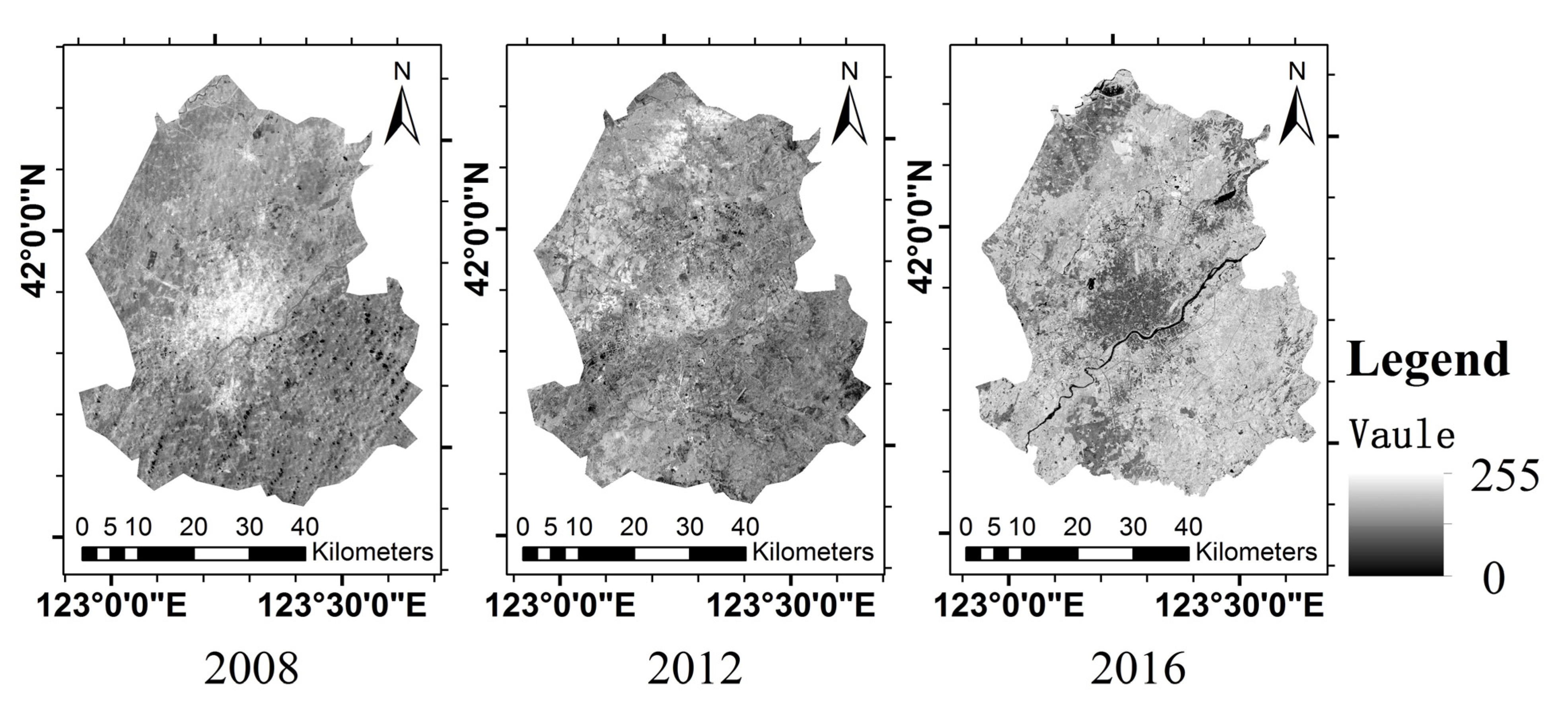
The Landsat images of 2008, 2012, and 2016 were pre-processed. NDISI index images were calculated and stretched to 0 to 255, and the stretched NDISI index images of Shenyang are shown in Figure 3. As we can see from Figure 3, the gray-scale value of the NDISI index image was proportional to the probability of belonging to the built-up area.
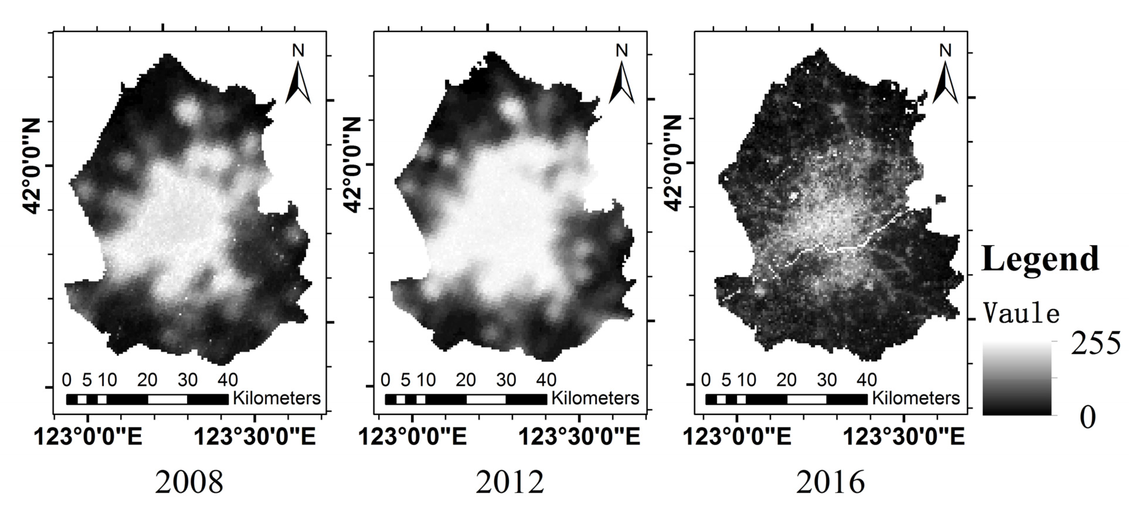
The DMSP/OLS images from 2008 and 2012 and the VIIRS/NPP images from 2016 were radiation corrected, and Shenyang night-time lighting images are shown in Figure 4.
The NDUBI index images were constructed by NDISI index images and night-time lighting images, and Shenyang NDUBI index images are shown in Figure 5. As shown in Figure 5, the character of the built-up area was enhanced significantly.
The statistics of government-declared built-up areas of central Liaoning urban agglomeration in 2008, 2012, and 2016 are shown in Table 1. Based on this, the optimal segmentation thresholds obtained by the statistical comparison method are also shown in Table 1. Between 2008 and 2016, the area of each city increased. The optimal segmentation thresholds for 2016 were significantly different from the remaining two years and had a sharp decrease due to the different sensors. Although NPP/VIIRS images’ range of brightness values were changed to be the same as DMSP/OLS, the results also were affected.
The NDUBI images were segmented by the optimal threshold. The built-up area extraction results are shown in Figure 6. The detailed step of the statistical comparison method to get the threshold is shown in Section 3.2.2. As shown in Figure 6, the spatial coverage of built-up areas had increased significantly in all cities. The growth of urban built-up areas showed two patterns: the core city of Shenyang had merged with smaller surrounding towns, such as small built-up areas in the north and south; the rest of the cities were multiregional developments, generally building development zones around the city, such as the small built-up areas that emerged in Fushun’s northeast region in 2016.
4.1.2. Accuracy Analysis of Built-Up Areas Extraction
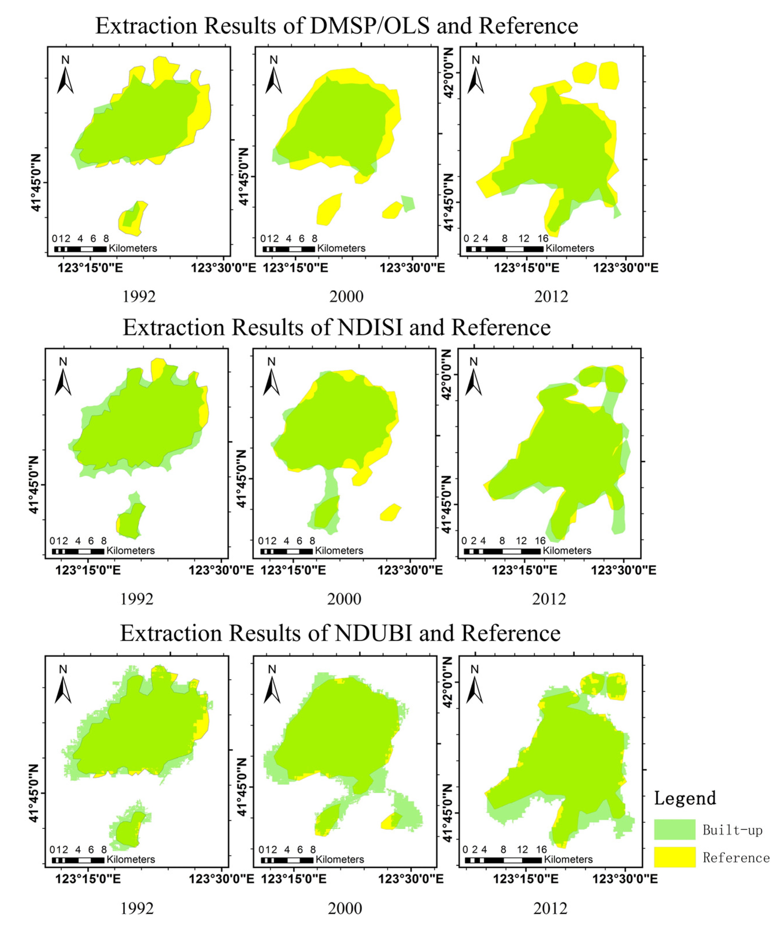
The extraction accuracy of built-up areas is the guarantee of the accurate extraction of urban axes. In this paper, the built-up area extraction method based on the normalized difference urban built-up area index was compared with the method by night-time lighting images or Landsat images. Shenyang was selected as the experimental area, DMSP/OLS data were selected for night-time lighting images. The method still used the statistical data comparison method. For Landsat data, the impervious surfaces of the city were first extracted, and the urban built-up areas were extracted by fusing small spots on this basis. The study time was selected for 1992, 2000, and 2012. The reason for choosing this time period was to compare the validity between the parameters and made the comparison results clearer. The control variables were different only for the methods, and the data types used should remain the same to avoid differences in the comparison of results due to transformed data source.
The optimal segmentation thresholds for night-time lighting images and NDUBI index images are shown in Table 2.
Since gray values of DMSP/OLS data were in the range of 0 to 63, the optimal segmentation thresholds were small. However, in order to unify the gray range of the impervious surface index image and the night-time lighting image, the gray values of NDUBI were stretched to 0 to 255, so the NDUBI segmentation thresholds were larger.
The build-up areas extraction results of the three methods are shown in Figure 7. The reference data were extracted artificially from Landsat data. The result areas of DMSP/OLS images were slightly smaller than the reference data, which meant that there was an omission in the extraction results of night-time lighting images. While the misclassification of extraction results of Landsat data was more obvious, the overall extraction results had good accuracy and no excessive disparity occurs. The results based on NDUBI index had a larger range compared with the reference data, but the overall extraction results were better.
In this paper, the Kappa coefficient, overall accuracy, user accuracy, and producer accuracy were evaluated by the confusion matrix, and the accuracy evaluation results are shown in Table 3. The kappa coefficients of the method based on DMSP/OLS data were able to maintain above 0.75, but none of the producer accuracy exceeded 0.75. The minimum values of Kappa coefficient and user accuracy for the method based on Landsat images are 0.77 and 0.74, with fluctuations in 2012. The method based on NDUBI index had the highest average Kappa coefficient and the Kappa coefficient did not fluctuate, reflecting the comprehensiveness. It showed that the results extracted by NDUBI index were more stable and less susceptible to data quality disturbances than the other two methods, and the accuracy was improved compared with the other
There are various methods to extract urban built-up areas, mainly using the large-scale characteristics of nighttime lighting data or the precision of Landsat data to obtain the results. In this paper, we compared the results obtained from nighttime lighting data and Landsat data with the proposed new index normalized difference urban built-up area index. The results showed that the index better solved the problems of the overflow of lights and the fragmentation of results caused by Landsat data, and achieved the extraction of urban built-up areas more quickly and efficiently while ensuring the accuracy of the extracted results for urban built-up areas, so that the information of urban built-up areas was significantly enhanced.
4.2. Urban Axes Extraction
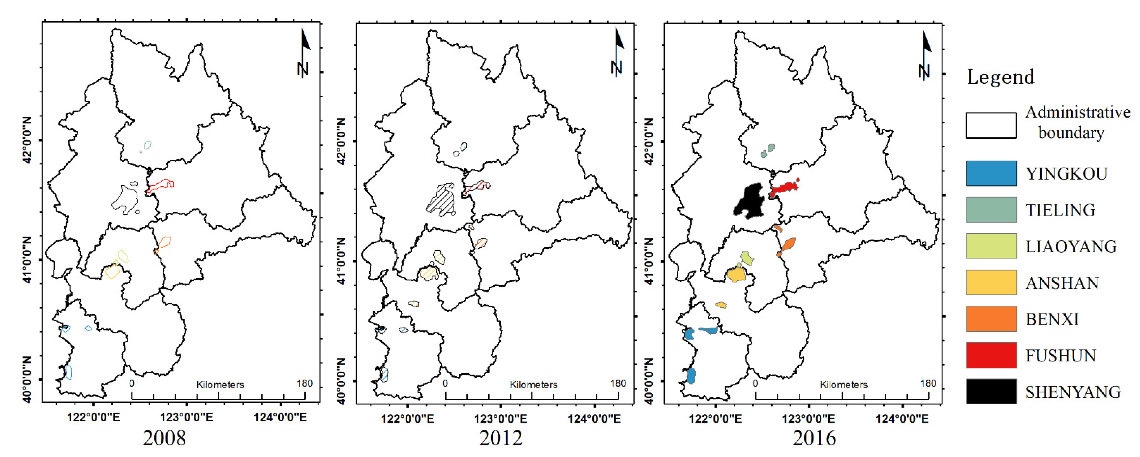
The Delaunay triangulation method was used to extract the urban axis of the built-up areas of central Liaoning urban agglomeration in 2008, 2012, and 2016, and the extraction results are shown in Figure 8. The period 2008 to 2016 was chosen because this time period was a period of rapid economic development in China, and urbanization was rapidly accelerating. Rapid urbanization had led to rapid inter-city linkages, making the experimental results more representative.
As shown in Figure 8, the urban axes accurately reflect the spatial characteristics of the built-up areas, including shape and direction of extension. It shows clearer than Figure 8 in the expansion direction. By comparing and analyzing the urban axes in the three years, it shows that the urban axes of Shenyang and Anshan have multiple directions, whereas the urban axis of the other cities have a single direction. For the core city like Shenyang, external expansion was not very obvious because it had already formed its own development pattern and was subject to regional restrictions. However, for the rest of the fast-growing cities, external expansion was evident. In Anshan, Benxi, and Fushun, while the city’s downtown was expanding, these cities were also developing new districts as built-up areas. And these new built-up areas would develop along the axes to the downtown, for example, Liaoyang and Tieling. In addition, we can see from the overall view that there is also a trend of mutual development between different cities like Anshan and Liaoyang.
4.3. Urban Gravity
4.3.1. Calculation on Gross Sizes of Cities
This paper used principal component analysis to calculate gross sizes of cities. Based on several parameters, a comprehensive model was calculated that is representative of the gross sizes of cities. The included parameters contained many socio-economic variables, urban development indicators, and so on, which explained different aspects of urban formation.
Two principal components, principal component 1 (PC1) and principal component 2(PC2), were identified from the statistics and a component matrix. The results are shown in Table 4. The component matrix is the initial factor load matrix, where each load quantity represents the correlation coefficient between the principal component and the corresponding variable. In PC1, it shows that all selected parameters, expect mean of gray values, have a strong correlation. The gross sizes were calculated by PC1 and PC2.
The PC1 and PC2 were used to calculate the gross sizes. The specific calculation procedure is shown in (6)–(7). For simplicity of results, the gross sizes were normalized by 2008 as the base year [26]. The final composite sizes of the central Liaoning urban agglomeration are shown in Table 5. According to the values of the obtained gross sizes of cities, we can make a ranking of the level. Since the principal components do not have a meaningful ratio scale, we cannot make a quantitative evaluation. The results were only used to describe the rank of the level of the development.
In Table 5, it shows that there is an indication of the level of development of cities. We used the obtained gross sizes to rank the level of development of cities in the urban agglomeration. It can be seen from the table that, in the three years, Shenyang, as the core city, was always the first one in the rank. Anshan, Fushun and Tieling also had stable rankings. Only Yingkou showed a steady growth. Liaoyang and Benxi both increased and decreased in ranking. We guess it may be that the overall development level of Liaoning is not high due to geographical factors and so on. The development of Yingkou was more obvious rise, since it was located at the transportation hub of two major cities in Liaoning, Shenyang, and Dalian. For the other cities, the changes were not obvious, since there were many resource-based cities with a single industrial structure and depleted resources [27].
4.3.2. Urban Gravity Calculation
The urban gravity models between the core city of central Liaoning urban agglomeration, Shenyang, and the rest of the cities were calculated, which the distances between cities were expressed as the distances between the closest endpoints on the urban axes. The urban gravity values and distance between cities are shown in Table 6. In Table 6, it shows that the gravity of Shenyang and Fushun is the largest, followed by Shenyang and Benxi, the urban gravity of Shenyang and rest cities is less than 1. The unit of distance is kilometers.
In Table 6, it shows that the interaction between Shenyang and Fushun is the closest. Geographically, the two cities are the closest in distance. The data in the table show a strong correlation with the distance between cities, which proves that the results are more related to spatial distance. In order to describe the relationship between cities more objectively, we used the change rate.
4.4. Integration Development Analyst of China Central Liaoning Urban Agglomeration
The change rates of gravity between Shenyang and other cities were calculated, and the results are shown in Table 7. In Table 7, when the value is positive, the gravitational force between cities keeps growing and, conversely, keeps declining. The table shows that there are higher urban gravitational growth rates between Shenyang and Fushun or Benxi, that Shenyang with Benxi reaching 143.07% from 2008 to 2012 and Shenyang with Fushun reaching 193.49% from 2012 to 2016. It indicated that the relationship of the two cities was highly closer. The urban gravity growth rate between Shenyang and Fushun or Yingkou increased, that means the city was more closely linked to the core city than in the previous year. Whereas the urban gravity growth rate between Shenyang and Tieling decreased. Although growth rates have declined, inter-city gravitational forces have still increased, just not to the same extent as in the previous year’s division. The urban gravity between Shenyang and Anshan or Liaoyang showed a tendency to decrease. At this point it meant that the gravitational force between the two cities was getting smaller and less connected.
The growth rates between most cities and Shenyang are not high and even on a downward trend, because Shenyang is not competitive as a core city and its radiation drive is limited [28]. Insufficient innovation has become an important factor limiting the development of central Liaoning urban agglomeration. Meanwhile, influenced by the slowdown of economic growth, low wage level and weak radiation-driving ability of cities, the net outflow of population from central Liaoning urban agglomeration has started since 2014, and the population outflow and aging aggravation have reduced the development momentum of urbanization. Due to the similar resource conditions and the same investment direction driven by the interests of enterprises, the industrial isomorphism of central Liaoning urban agglomeration is serious. Petrochemical, iron and steel, energy and equipment manufacturing have become the key development industries of most cities. Because of the serious duplication of industries, it is difficult to realize the cluster effect, resulting in a large waste of resources and unable to cultivate brand competitiveness.
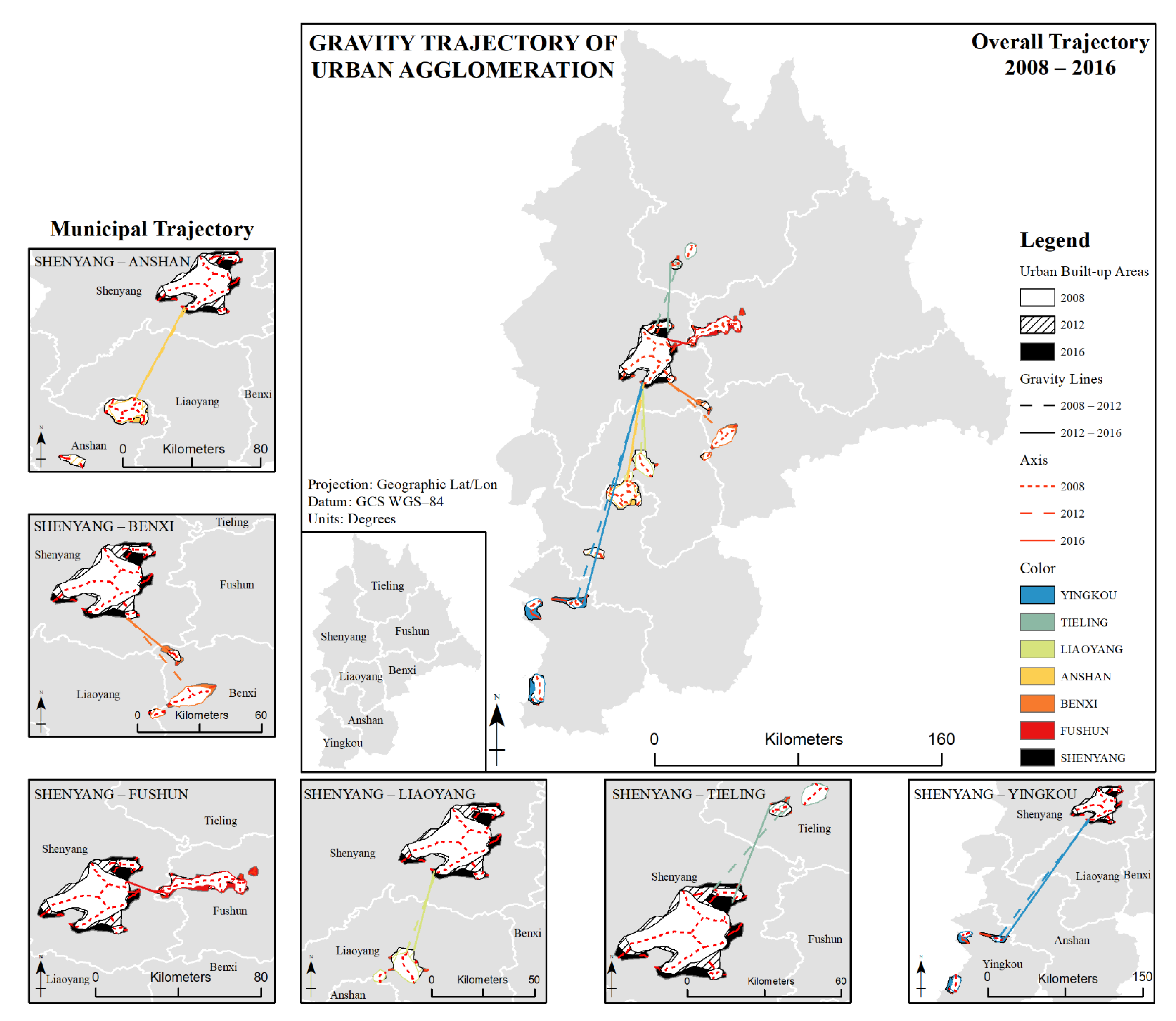
The multitemporal urban axes were extracted as the urban gravity trajectory, and the urban gravity trajectory of central Liaoning urban agglomeration is shown in Figure 9. The connections between different cities in different years were distinguished according to style and color. The development direction of the built-up area in the next study period tended to be roughly the same as that of the inter-city linkage. Therefore, we could infer that there was a correlation between the development of the city and the direction of gravitational force.
As seen from Figure 9, the spatial variation trend of urban axes reflected the urban gravity trajectory. The connecting lines between Shenyang and Fushun were getting shorter and shorter. And Fushun had developed along the Hunhe River to the west. The trend was the same between Shenyang and Benxi. Benxi Development Zone was developing to the northwest, bordering Shenyang’s Hunnan District. Anshan, Liaoyang, and Yingkou also had the tendency to develop towards Shenyang, but the gravity trajectories changed little. Because of the poor development of Tieling, there was no significant inter-city development.
In summary, from the results of gravitational strength and gravitational trajectory changes, it can be seen that, except for Fushun and Benxi, the connections between the rest of the cities and Shenyang were not significantly strengthened, and the integration of central Liaoning urban agglomeration was weak.
4.5. Correlation Analysis of Urban Gravitational Direction Lines and Urban Gravitational Trajectories
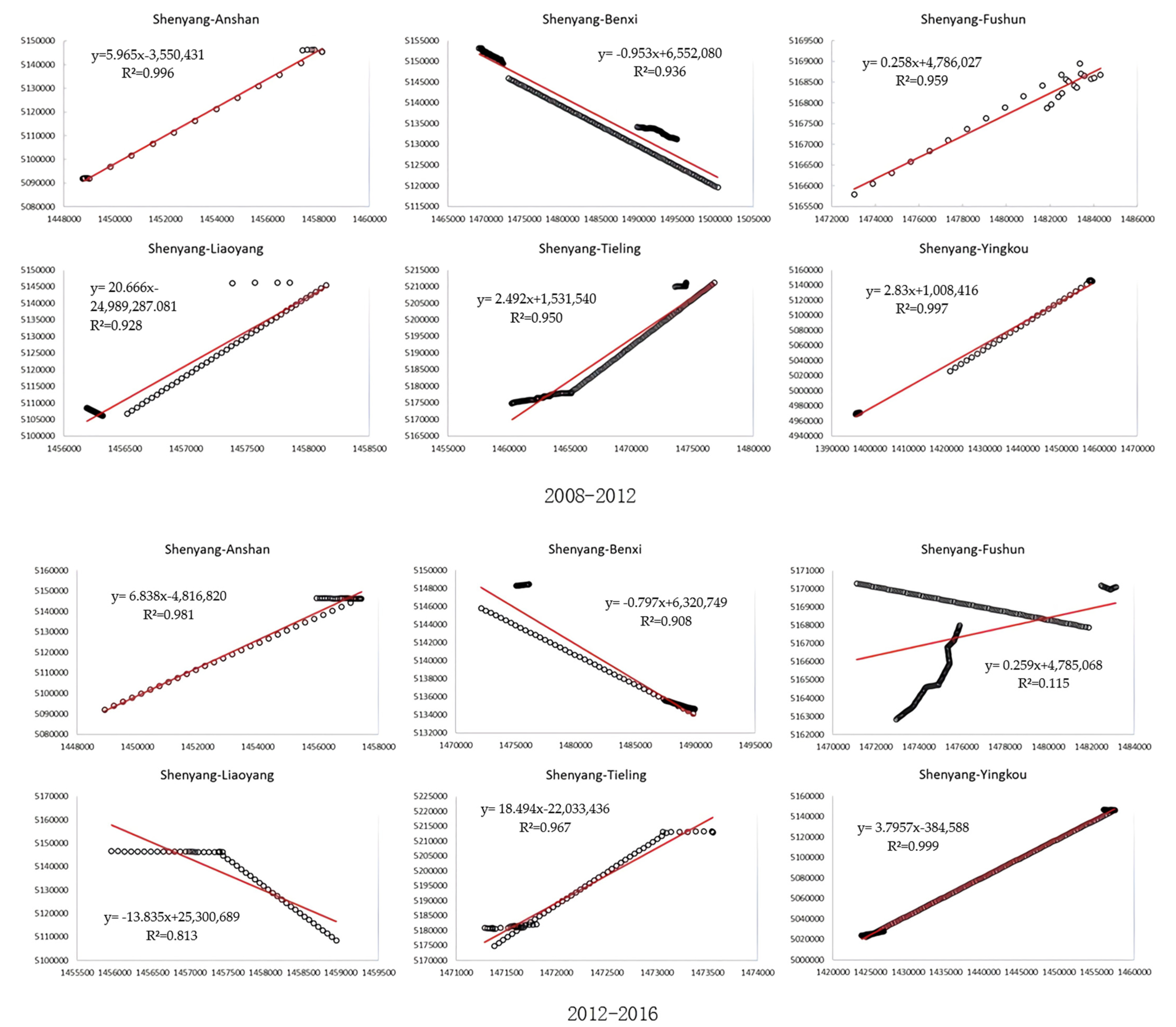
There is gravitational direction between objects, such as the gravitational direction towards the center of the earth. In this paper, the gravitational direction lines were the connecting lines between the endpoints of the urban axes. To demonstrate the validity of using the trend of urban axes as the gravitational trajectory of the city, it was verified by analyzing the correlation between the gravitational trajectory and the gravitational direction line. Firstly, we took points equidistant from two cities to form the set of urban axis points and the set of gravitational direction line points. Then, the correlation of the two kinds of point sets was analyzed. Finally, the correlation between the two data sets was analyzed by correlation coefficient. The correlation analysis results of urban gravitational trajectory and urban gravitational direction line are shown in Figure 10.
It can be seen from Figure 10 that, except for Shenyang and Fushun from 2012 to 2016, the correlation coefficients between Shenyang and other cities were above 0.75. When the values above 0.75, it means that the two for analysis have the strong correlation. However, for the result of Shenyang and Fushun from 2012 to 2016, the correlation coefficient is 0.115, indicating that the correlation is not strong. It can be seen through Figure 8 that there is an internal conjunctive development trend between the northeast corners of the city in Shenyang in 2012, which makes the axial direction change. This may be the reason for this particular result. However, a discrete result does not affect the overall result. In addition, the fits of the two-point sets were generally good, indicating that the trend of urban axis change is strongly correlated with the urban gravity direction line. Therefore, the trend of urban axis change can describe the urban gravity trajectory.
Meanwhile, since Liaoning is an old industrial province, the main industries of several cities in the province are industrial. In China, most northern industrial cities are facing the challenge of urban transformation. The policymakers and city authorities are exploring solutions to provide new services to large populations in an efficient, responsive, and sustainable manner. Current urbanization requires strong strategies and innovative planning to modernize urban life [29]. But the rapid development of energy efficiency programs in commercial buildings over the past decade can lead to a growing decoupling effect [30]. It is therefore normal for some of these cities to identify a range of services and prioritize demand in order to obtain user value for a long-term urban transformation that will accelerate their own development and a certain decoupling from the development of the core city.
5. Conclusions
This paper validated the effectiveness of the proposed urban trajectory gravity model by analyzing integration development of central Liaoning urban agglomeration. By analyzing the gravity of core city in urban agglomeration to other cities, the relationship between urban spatial change and gravity was established. Different from the traditional urban gravity model, which only provides urban gravitational strength, this paper gives the spatial description of gravity. It can determine the change characteristics of gravity direction, extension, or contraction, so that the description of urban agglomeration integration development has an objective basis to follow.
5.1. Key Findings
This paper presented the normalized differential urban built-up area index combining night-time lighting data and Landsat data. The method can be used to quickly extract urban built-up areas, improve the incomplete information representation of built-up areas by single source data, and increase the accuracy of built-up area extraction. In order to describe the strength and trajectory of urban gravity, the urban gravity trajectory model was proposed. The model adopted the indicators including urban information, population, and economy to calculate urban gravity, and described the urban gravitational trajectory through the changes of multitemporal urban axis, which could provide a more comprehensive and objective analysis of the integrated development of urban agglomeration.
The results show that cities are constantly attracted to each other through urban gravity. For the different cities in the same year, a higher correction coefficient of fitting analysis means a stronger relationship. There is a clear gravitational force between the cities when the value above 0.75. For the most cities in different years, the gravitational force between the core city with itself is increasing by years. At the same time, the direction of growth of the urban axes tends to increase in the direction of the gravitational force between cities. There is a clear tendency for the trajectories of the cities to move closer together.
5.2. Future Work
A central city, with its expanding scale and growing strength, will have a radiating effect on the surrounding areas. Along with the continuous improvement of inter-city transportation conditions, the radiation belts between neighboring cities are increasing, and even overlap phenomenon occurs. In this paper, we can see that China’s urban agglomerations are gradually developing, and the old industrial cities represented by the central Liaoning urban agglomeration are also in the process. The cities are gradually transformed by various factors such as urban infrastructure, transportation, and population. This paper analyzes the drivers of inter-city cluster development, starting from the direction of inter-city cluster development.
This paper still has some shortcomings. The statistical comparison method uses the built-up area of government statistics to determine the optimal segmentation threshold of NDUBI index image. The social science data used to calculate gross sizes of cities is mainly from government statistics. These data sources have been criticized due to its nonobjectivity and low quality. In addition, the variables we use for PCA, which represent absolute measures, assess more the size of a city than the actual level of urbanization.
Additionally, for the next study, social media data such as POI data and weibo check-in data may improve the objectivity of the data. Furthermore, in order to determine the level of urbanization, it would be better to use relative measures rather than absolute measures. Finally, we can analyze the role played by different kinds of cities, such as industrial cities, trading cities, etc., in urban agglomerations and their drivers from the perspective of city types and development structures.
Author Contributions
Conceptualization, Zhiwei Xie; methodology, Shoujia Li; writing—original draft preparation, Shoujia Li; writing—review and editing, Ruren Li; funding acquisition, Zhiwei Xie. All authors have read and agreed to the published version of the manuscript.
Funding
This work was funded by Economic and Social Development Research Project of Liaoning Province (CN) (No.2021lslqnkt-010.), Education Department Scientific Research Project of Liaoning Province (CN) (No. lnqn201917), National Natural Science Foundation of China (No.4210010785) and Humanities and Social Science Foundation of the Ministry of Education (CN) (No.21YJC790129).
Institutional Review Board Statement
Not applicable.
Informed Consent Statement
Not applicable.
Conflicts of Interest
The authors declare no conflict of interest.
References
- Duranton, G.; Puga, D. Micro foundations of Urban Agglomeration Economies. Soc. Sci. Electron. Pub. 2003, 4, 2063–2117. [Google Scholar]
- Fang, C.; Yu, D. Urban agglomeration: An evolving concept of an emerging phenomenon. Landsc. Urban. Plan. 2017, 162, 126–136. [Google Scholar] [CrossRef]
- Lin, W.; Wu, M.; Zhang, Y.; Zeng, R.; Zheng, X.; Shao, L.; Zhao, L.; Li, S.; Tang, Y. Regional differences of urbanization in China and its driving factors. Sci. China Earth Sci. 2018, 61, 778–791. [Google Scholar] [CrossRef]
- Xu, F.; Chi, G. Spatiotemporal variations of land use intensity and its driving forces in China, 2000–2010. Reg. Environ. Chang. 2019, 19, 2583–2596. [Google Scholar] [CrossRef]
- Peng, J.; Lin, H.; Chen, Y.; Blaschke, T.; Luo, L.; Xu, Z.; Hu, Y.; Zhao, M.; Wu, J. Spatiotemporal evolution of urban agglomerations in China during 2000–2012: A nighttime light approach. Landsc. Ecol. 2020, 35, 421–434. [Google Scholar] [CrossRef]
- Zhang, X.N.; Wang, W.W.; Harris, R.; Leckie, G. Analysing inter-provincial urban migration flows in China: A new multilevel gravity model approach. Migr. Stud. 2018. [Google Scholar] [CrossRef]
- Chen, Y.; Huang, L. A scaling approach to evaluating the distance exponent of the urban gravity model. Chaos Solitons Fractals 2018, 109, 303–313. [Google Scholar] [CrossRef] [Green Version]
- Burger, M.; Van Oort, F.; Meijers, E. Examining Spatial Structure Using Gravity Models. Introd. Contin. Time Stoch. Process. 2019, 471–479. [Google Scholar] [CrossRef]
- Aboelnaga, S.; Toth, T.; Neszmelyi, G.I. Land use management along urban axis as one of urban regeneration principles. In Proceedings of the 18th International Scientific Conference on Engineering for Rural Development (ERD), Jelgava, Latvia, 22–24 May 2019; pp. 944–953. [Google Scholar] [CrossRef]
- Imhoff, M.L.; Lawrence, W.T.; Stutzer, D.C.; Elvidge, C.D. A technique for using composite DMSP/OLS “City Lights” satellite data to map urban area. Remote Sens. Environ. 1997, 61, 361–370. [Google Scholar] [CrossRef]
- Yu, B.; Tang, M.; Wu, Q.; Yang, C.; Deng, S.; Shi, K.; Peng, C.; Wu, J.; Chen, Z. Urban Built-Up Area Extraction From Log- Transformed NPP-VIIRS Nighttime Light Composite Data. IEEE Geosci. Remote Sens. Lett. 2018, 15, 1279–1283. [Google Scholar] [CrossRef]
- Liu, X.; Wu, Y.; Hu, H. A method of extracting multiscale skeletons for polygonal shapes. Acta Geod. Cartograph. Sin. 2013, 42, 588–594. [Google Scholar]
- Miao, Z.; Baležentis, T.; Tian, Z.; Shao, S.; Geng, Y.; Wu, R. Environmental Performance and Regulation Effect of China’s Atmospheric Pollutant Emissions: Evidence from Three Regions and Ten Urban Agglomerations. Environ. Resour. Econ. 2019, 74, 211–242. [Google Scholar] [CrossRef]
- Cao, S.; Hu, D.; Zhao, W.J.; Mo, Y.; Yu, C.; Zhang, Y. Monitoring changes in the impervious surfaces of urban functional zones using multisource remote sensing data: A case study of Tianjin, China. GISci. Remote Sens. 2019, 56, 967–987. [Google Scholar] [CrossRef]
- Lu, D.; Weng, Q. Use of impervious surface in urban land-use classification. Remote Sens. Environ. 2006, 102, 146–160. [Google Scholar] [CrossRef]
- Sun, Z.; Wang, C.; Guo, H.; Shang, R. A Modified Normalized Difference Impervious Surface Index (MNDISI) for Automatic Urban Mapping from Landsat Imagery. Remote Sens. 2017, 9, 942. [Google Scholar] [CrossRef] [Green Version]
- Shen, Z.; Zhu, Y.; Cao, Y.; Chen, J. Measurement of blooming effect of DMSP-OLS nighttime light data based on NPP-VIIRS data. Annal. GIS 2019, 25, 153–165. [Google Scholar] [CrossRef] [Green Version]
- He, C.; Shi, P.; Li, J.; Chen, J.; Pan, Y.; Li, J.; Zhuo, L.; Ichinose , T. A Study on the Reconstruction of the Spatial Process of Urbanization in 1990s in Mainland China Based on DMSP/OLS Night Light Data and Statistical Data. Chin. Sci. Bull. 2006, 51, 856–861. [Google Scholar] [CrossRef]
- Yao, Y.; Chen, D.; Chen, L.; Wang, H.; Guan, Q. A time series of urban extent in China using DSMP/OLS nighttime light data. PLoS ONE 2018, 13, e0198189. [Google Scholar] [CrossRef] [Green Version]
- Xie, Z.; Ye, X.; Zheng, Z.; Li, D.; Sun, L.; Li, R.; Benya, S. Modeling Polycentric Urbanization Using Multisource Big Geospatial Data. Remote Sens. 2019, 11, 310. [Google Scholar] [CrossRef] [Green Version]
- Jiang, Z.; Zhai, W.; Meng, X.; Long, Y. Identifying Shrinking Cities with NPP-VIIRS Nightlight Data in China. J. Urban. Plan. Dev. 2020, 146, 04020034. [Google Scholar] [CrossRef]
- Elvidge, C.; Sutton, P.; Baugh, K.E.; Ziskin, D.; Tilottama, D.; Anderson, S. National Trends in Satellite Observed Lighting: 1992–2009. AGU Fall Meet. Abstr. 2011, 3, 357. [Google Scholar]
- Zhang, Q. Spatial Expansion of New First-tier Cities Using the DMSP/OLS Nighttime Light Images. J. Geomat. 2015, 40, 72–75. [Google Scholar]
- Shu, S.; Yu, B.; Wu, J.; Liu, H. Methods for Deriving Urban Built-up Area Using Night-light Data: Assessment and Application. Remote Sens. Technol. Appl. 2011, 26, 169–176. [Google Scholar]
- Liu, Y.; Lu, S.; Chen, Y. Spatio-temporal change of urban–rural equalized development patterns in China and its driving factors. J. Rural. Stud. 2013, 32, 320–330. [Google Scholar] [CrossRef]
- Li, M.; Chen, M.; Chen, Y. Study on Target Standardization Method of Comprehensive Evaluation in Chinese. J. Manag. Sci. 2004, 12, 45–48. [Google Scholar]
- Wang, F. Research on the Development of Continuous Industry in Resource based City—Taking Liaoning Province as an example. J. Shenyang Univ. 2020, 22, 172–175. [Google Scholar]
- Ma, T.; Wei, J.; Liang, T. Countermeasures for the Development of South-Central Liaoning City Cluster under the New Re-gional Development Pattern. J. Bohai Univ. 2020, 42, 78–82. [Google Scholar]
- Harish, K.; Manoj Kumar, S.M.P.G.; Jitendra, M. Moving towards smart cities: Solutions that lead to the Smart City Trans-formation Framework. Technol. Forecast. Soc. Chang. 2020, 153, 119281. [Google Scholar]
- Mma, B.; Wei, C.; Weiguang, C.; Dong, L. Whether carbon intensity in the commercial building sector decouples from economic development in the service industry? Empirical evidence from the top five urban agglomerations in China. J. Clean. Prod. 2019, 222, 193–205. [Google Scholar] [CrossRef]
Figure 1.
Location of China Central Liaoning urban agglomeration.

Figure 2.
(a) Classification of triangles in the Delaunay triangle network; (b) skeletal lines of faceted elements.
Figure 2.
(a) Classification of triangles in the Delaunay triangle network; (b) skeletal lines of faceted elements.

Figure 3.
Shenyang NDISI index image.

Figure 4.
Shenyang night-time lighting images after radiation correction.

Figure 5.
Shenyang NDUBI images.

Figure 6.
Built-up area of central Liaoning urban agglomeration.

Figure 7.
The build-up areas extraction results of the three methods.

Figure 8.
Urban axis of central Liaoning urban agglomeration.

Figure 9.
Gravity trajectory of central Liaoning urban agglomeration.

Figure 10.
The correlation analysis results of urban gravitational trajectory and urban gravitational direction line.
Figure 10.
The correlation analysis results of urban gravitational trajectory and urban gravitational direction line.


Table 1.
Statistical data of urban built-up areas (km2) and optimal segmentation threshold of central Liaoning urban agglomeration.
Table 1.
Statistical data of urban built-up areas (km2) and optimal segmentation threshold of central Liaoning urban agglomeration.
| Statistic Data | Segmentation Threshold | |||||
|---|---|---|---|---|---|---|
| Year | 2008 | 2012 | 2016 | 2008 | 2012 | 2016 |
| Shenyang | 370.00 | 455.00 | 588.26 | 137 | 157 | 18 |
| Anshan | 148.04 | 166.55 | 172.05 | 151 | 163 | 48 |
| Benxi | 106.50 | 108.00 | 109.00 | 211 | 222 | 30 |
| Fushun | 123.90 | 131.03 | 139.34 | 151 | 163 | 9 |
| Liaoyang | 66.00 | 76.50 | 76.50 | 149 | 149 | 30 |
| Tieling | 43.69 | 45.08 | 56.81 | 107 | 141 | 12 |
| Yingkou | 97.12 | 103.81 | 188.80 | 154 | 183 | 11 |
Table 2.
The optimal segmentation thresholds for nighttime light images and NDUBI index images.
| Item | 1992 | 2000 | 2012 |
|---|---|---|---|
| nighttime light images | 53 | 59 | 60 |
| NDUBI index images | 138 | 138 | 151 |
Table 3.
The accuracy evaluation results of built-up area extraction method.
| Accuracy Index 1 | DMSP/OLS | Impervious Surface | NDUBI | |||||||||
|---|---|---|---|---|---|---|---|---|---|---|---|---|
| 1992 | 2000 | 2012 | Mean | 1992 | 2000 | 2012 | Mean | 1992 | 2000 | 2012 | Mean | |
| K | 0.82 | 0.78 | 0.78 | 0.79 | 0.87 | 0.84 | 0.77 | 0.83 | 0.84 | 0.84 | 0.84 | 0.84 |
| OA | 0.98 | 0.96 | 0.95 | 0.96 | 0.98 | 0.98 | 0.99 | 0.98 | 0.98 | 0.97 | 0.95 | 0.97 |
| UA | 0.94 | 0.95 | 0.94 | 0.94 | 0.83 | 0.91 | 0.74 | 0.82 | 0.81 | 0.87 | 0.84 | 0.84 |
| PA | 0.75 | 0.68 | 0.70 | 0.71 | 0.94 | 0.84 | 0.98 | 0.92 | 0.89 | 0.85 | 0.91 | 0.88 |
1 K: Kappa coefficient; OA: Overall accuracy; UA: User accuracy; PA: Producer accuracy.
Table 4.
Component matrix in 2008, 2012, and 2016.
| Item | 2008 | 2012 | 2016 | |||
|---|---|---|---|---|---|---|
| PC 1 | PC 2 | PC 1 | PC 2 | PC 1 | PC 2 | |
| Sum of gray values | 0.926 | 0.370 | 0.943 | 0.313 | 0.970 | 0.237 |
| Mean of gray values | −0.149 | 0.972 | −0.263 | 0.947 | 0.088 | 0.992 |
| Built-up area | 0.985 | 0.133 | 0.987 | 0.116 | 0.992 | 0.004 |
| Added value of primary sector | 0.839 | −0.408 | 0.848 | −0.402 | 0.903 | −0.177 |
| Added value of secondary sector | 0.987 | 0.056 | 0.993 | 0.083 | 0.996 | 0.012 |
| Added value of tertiary sector | 0.994 | −0.002 | 0.993 | 0.062 | 0.998 | −0.011 |
| Population | 0.987 | 0.056 | 0.990 | 0.052 | 0.989 | 0.129 |
| Streetlights number | 0.949 | −0.036 | 0.964 | −0.032 | 0.917 | −0.318 |
| Urban road area | 0.996 | −0.060 | 0.990 | 0.016 | 0.996 | 0.002 |
| Variance value | 7.452 | 1.426 | 11.735 | 3.846 | 10.659 | 2.164 |
Table 5.
Gross sizes of cities.
| City | 2008 | Rank | 2012 | Rank | 2016 | Rank |
|---|---|---|---|---|---|---|
| Shenyang | 1 | 1 | 1.024 | 1 | 1.036 | 1 |
| Anshan | 0.284 | 2 | 0.272 | 2 | 0.205 | 2 |
| Benxi | 0.140 | 4 | 0.107 | 6 | 0.102 | 5 |
| Fushun | 0.147 | 3 | 0.128 | 3 | 0.146 | 3 |
| Liaoyang | 0.112 | 5 | 0.111 | 4 | 0.077 | 6 |
| Tieling | 0.037 | 7 | 0.048 | 7 | 0.033 | 7 |
| Yingkou | 0.105 | 6 | 0.110 | 5 | 0.145 | 4 |
Table 6.
The urban gravity and distance between cities in central Liaoning urban agglomeration.
| Cities | 2008 | 2012 | 2016 | |||
|---|---|---|---|---|---|---|
| Gravity | Distance | Gravity | Distance | Gravity | Distance | |
| Shengyang to Anshan | 0.963 | 54.295 | 0.931 | 54.619 | 0.704 | 54.918 |
| Shengyang to Benxi | 1.003 | 37.927 | 2.438 | 21.200 | 3.592 | 17.152 |
| Shengyang to Fushun | 9.758 | 10.817 | 10.777 | 11.028 | 31.629 | 6.915 |
| Shengyang to Liaoyang | 0.745 | 38.763 | 0.801 | 37.665 | 0.533 | 38.680 |
| Shengyang to Tieling | 0.304 | 34.788 | 0.342 | 37.919 | 0.369 | 30.447 |
| Shengyang to Yingkou | 0.067 | 125.105 | 0.068 | 128.257 | 0.101 | 122.085 |
Table 7.
Urban gravity change rate of central Liaoning urban agglomeration.
| Year | 2008 to 2012 | 2012 to 2016 |
|---|---|---|
| Shengyang to Anshan | −3.32% | −24.38% |
| Shengyang to Benxi | 143.07% | 47.33% |
| Shengyang to Fushun | 10.44% | 193.49% |
| Shengyang to Liaoyang | 7.52% | −33.46% |
| Shengyang to Tieling | 12.50% | 7.89% |
Publisher’s Note: MDPI stays neutral with regard to jurisdictional claims in published maps and institutional affiliations. |
© 2021 by the authors. Licensee MDPI, Basel, Switzerland. This article is an open access article distributed under the terms and conditions of the Creative Commons Attribution (CC BY) license (https://creativecommons.org/licenses/by/4.0/).
Share and Cite
MDPI and ACS Style
Li, R.; Li, S.; Xie, Z. Integration Development of Urban Agglomeration in Central Liaoning, China, by Trajectory Gravity Model. ISPRS Int. J. Geo-Inf. 2021, 10, 698. https://0-doi-org.brum.beds.ac.uk/10.3390/ijgi10100698
AMA Style
Li R, Li S, Xie Z. Integration Development of Urban Agglomeration in Central Liaoning, China, by Trajectory Gravity Model. ISPRS International Journal of Geo-Information. 2021; 10(10):698. https://0-doi-org.brum.beds.ac.uk/10.3390/ijgi10100698
Chicago/Turabian StyleLi, Ruren, Shoujia Li, and Zhiwei Xie. 2021. "Integration Development of Urban Agglomeration in Central Liaoning, China, by Trajectory Gravity Model" ISPRS International Journal of Geo-Information 10, no. 10: 698. https://0-doi-org.brum.beds.ac.uk/10.3390/ijgi10100698
Note that from the first issue of 2016, this journal uses article numbers instead of page numbers. See further details here.