The Integration of GPS/BDS Real-Time Kinematic Positioning and Visual–Inertial Odometry Based on Smartphones

Abstract

The real-time kinematic positioning technique (RTK) and visual–inertial odometry (VIO) are both promising positioning technologies. However, RTK degrades in GNSS-hostile areas, where global navigation satellite system (GNSS) signals are reflected and blocked, while VIO is affected by long-term drift. The integration of RTK and VIO can improve the accuracy and robustness of positioning. In recent years, smartphones equipped with multiple sensors have become commodities and can provide measurements for integrating RTK and VIO. This paper verifies the feasibility of integrating RTK and VIO using smartphones, and we propose an improved algorithm to integrate RTK and VIO with better performance. We began by developing an Android smartphone application for data collection and then wrote a Python program to convert the data to a robot operating system (ROS) bag. Next, we established two ROS nodes to calculate the RTK results and accomplish the integration. Finally, we conducted experiments in urban areas to assess the integration of RTK and VIO based on smartphones. The results demonstrate that the integration improves the accuracy and robustness of positioning and that our improved algorithm reduces altitude deviation. Our work can aid navigation and positioning research, which is the reason why we open source the majority of the codes at our GitHub.

1. Introduction

Global navigation satellite systems (GNSSs) have advanced at a breakneck pace in recent years. The expansion of constellations, as well as the addition of new signals and the introduction of multiple positioning solutions, have contributed to the advancement of precise navigation [1,2]. The real-time kinematic positioning technique (RTK) is representative and attracts research. RTK is a differential positioning technique that utilizes at least one stationary station to determine the location of movable receivers. The stationary station, also known as the reference station, is critical for providing a reference and mitigating common errors between itself and the movable receiver, also known as the rover or the user [3]. RTK simultaneously processes the pseudo-range and carrier phase measurements with the ambiguity resolution (AR) technique to generate more accurate positioning results [4]. According to certain studies, the dual-frequency RTK can accomplish quick AR for short baselines, resulting in real-time centimeter-level precision [5]. In comparison, the single-frequency RTK performance is restricted but can be considerably improved by utilizing satellites from various constellations. These constellations include the global positioning system (GPS), the China-developed Beidou navigation satellite system (BDS), the European Galileo system, and the Russian global navigation satellite system (GLONASS) [6,7,8]. RTKLIB is a well known and representative open-source software for calculating RTK positioning results [9].

Compared to geodetic-grade multifrequency GNSS receivers, consumer-grade receivers are more prevalent in everyday life because of their low cost and low-power consumption. Smartphones, which have become almost ubiquitous in modern society, can be thought of as consumer-grade GNSS receivers. However, smartphone-grade antennas might lose several or even dozens of decibels of sensitivity when compared to professional GNSS antennas, causing smartphones to struggle to maintain a lock on GNSS signals [10]. Additionally, GNSS signals are circularly polarized to suppress the effect of Faraday rotation, while smartphone-grade antennas adopt linear polarization [11]. As a result, the smartphone-grade antenna can only provide a poor carrier-to-noise ratio and insufficient multipath suppression, limiting the performance of the smartphone’s built-in GNSS receiver [12]. The advancement of the Android operating system and GNSS chipsets promotes research into positioning, using smartphones. Before 2016, researchers could only obtain the positioning results calculated by the inbuilt GNSS chipset. This situation persisted until Google released Android N, which started providing the Android Raw GNSS Measurements API. Since then, developers have gained access to the pseudo-range and carrier phase measurements and have begun processing the measurements, using their positioning algorithms [13]. Nonetheless, a technique called duty cycling prevents smartphones from tracking the carrier phase continuously. Duty-cycling periodically powers on and off the GNSS chipset to extend the battery life [14]. Android P has a developer option titled “Force full GNSS measurements” that disables duty cycling, paving the path for precise positioning with the carrier phase [15]. Meanwhile, the Xiaomi MI 8 equipped with BCM47755 was released. The Xiaomi MI 8 can provide dual-frequency GNSS measurements and has become an ideal platform for research into smartphone-based precise positioning. According to studies, the Xiaomi MI 8 is promising for offering accurate positioning results in urban areas with RTK and precise point positioning (PPP) [16,17,18].

Users of smartphones are often pedestrians in urban areas. Buildings can block and reflect GNSS signals, obstructing receivers’ ability to maintain signal tracking and exacerbating the multipath effect. The carrier phase tracking loop is the weakest link of the GNSS receiver, and it is easier that the carrier tracking loop loses the lock than the code tracking loop [19,20]. 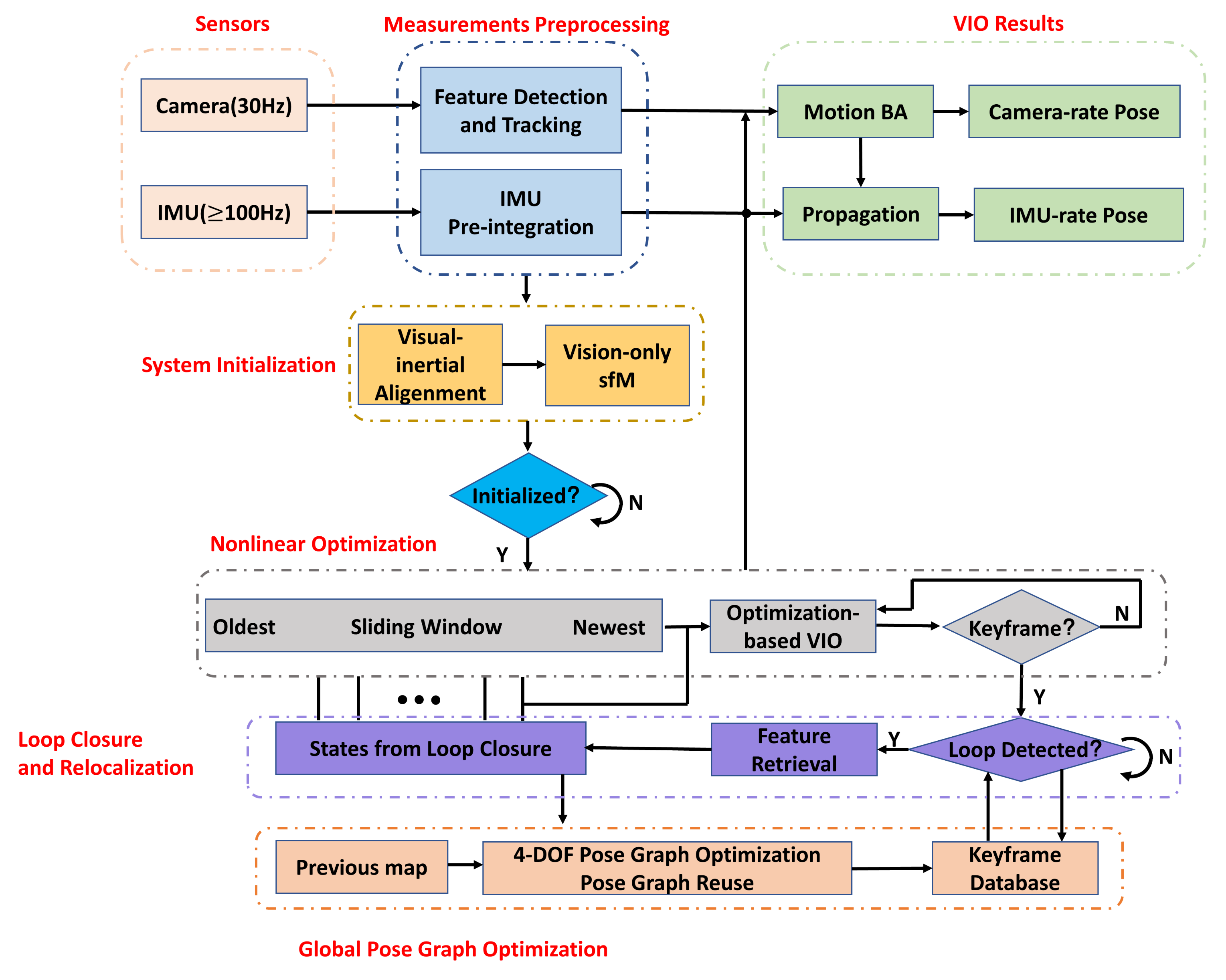The carrier phase measurements may occasionally be absent in urban areas [21]. A pedestrian often keeps their smartphone near their body when they need positioning. As a result, the user’s body becomes an unavoidable signal blocker. This fact significantly constrains the performance of smartphone-based RTK. We should introduce other sensors and positioning approaches to assist RTK in providing continuous positioning results in urban areas. A common complementary solution is the inertial navigation system (INS) based on an inertial measurement unit (IMU) [22]. An IMU consists of gyroscopes and accelerometers. The measurements are subject to additive noise and a changing bias, which results in a long-term drift in positioning [23]. Visual odometry (VO), a camera-based visual approach, is also a supplementary positioning solution [24]. VO performance is constrained by light circumstances, ambient textures, and device speed. In the case of monocular VO, the system’s absolute scale is ambiguous [25]. Visual–inertial odometry (VIO) is a technique that combines VO with INS to mitigate long-term drift and solve scale ambiguity. Additionally, the combination increases the robustness [26]. VINS-mono, ORB-SLAM3, and MSCKF are representative VIO algorithms [27,28,29]. Generally, these algorithms are integrated with the robotic operating system (ROS) [30]. Nonetheless, VIO systems still undergo long-term drift [31]. In addition, VIO generates a pose output that includes the estimation of position and orientation in local coordinates, indicating that it is a relative positioning technique. Its positioning results depend on the starting point. As a result, VIO is unfriendly for reusing without a fixed global coordinate [32]. These positioning techniques are summarized in

Table 1. The comparison of different positioning techniques.

	Techniques	RTK	INS	VO	VIO
Features
Absolute positioning results		√	×	×	×
Long-term drifts		×	√	√	√
Scale ambiguity		×	×	√	×
Constraints		Signal blockage	IMU biases	Light Ambient textures Device’s speed	Light Ambient textures IMU biases

. In Table 1, √ means that the technique has a corresponding feature, while × means the opposite.

VIO can produce highly accurate relative positioning data in a short period of time. In contrast, GNSS positioning techniques can deliver absolute positioning results. Combining VIO and GNSS can provide locally accurate and global drift-free positioning results. In recent years, the integration of INS, VO, and GNSS has been a popular topic. ETH Zurich designed MSF-EKF, a loosely coupled GNSS/INS/VO framework, based on an extended Kalman filter (EKF) [33]. Rui Sun et al. proposed a GNSS/INS/VO fusion scheme, using two EKFs with a non-holonomic constraint (NHC) for real-time 3D vehicle state estimation [34]. Tong Qin and colleagues published VINS-fusion, a loosely coupled GNSS/VIO system based on optimization [35]. Tuan Li and his colleagues utilized MSCKF to tightly fuse RTK/INS/VO to increase velocity and attitude accuracy [36]. Shaozu Cao’s team offered GVINS, derived from VINS-mono. GVINS optimizes GNSS measurements, including pseudo-range and Doppler measurements, along with visual and inertial measurements [37]. These studies advance the field of navigation study. They focus on giving precise positioning results, using bulky and complex specialized devices. Additionally, researchers frequently need to assemble and synchronize sensors, as few commercial devices simultaneously collect GNSS measurements, inertial measurements, and images. For instance, VINS-fusion is built on a self-developed suite that contains stereo cameras and a DJI A3 controller (http://www.dji.com/a3 (accessed on 14 October 2021)). The DJI A3 controller comprises an IMU and a GNSS receiver. The team proposing GVINS combines a u-blox ZED-F9P receiver (https://www.u-blox.com/en/product/zed-f9p-module (accessed on 14 October 2021)) with a VI-Sensor [38]. The VI-Sensor synchronizes the camera and IMU well, and the ZED-F9P delivers a pulse per second (PPS) signal to trigger the VI-Sensor and align the time. Regrettably, the VI-Sensor is no longer commercially available (https://github.com/ethz-asl/libvisensor/issues/11 (accessed on 14 October 2021)). Rui Sun and Tuan Li both utilized three components to acquire GNSS measurements, IMU measurements, and images. They used the PPS signal to trigger the camera and record the GPS time of the exposure. These works are summarized in

Table 2. Works on the fusion of GNSS/IMU/VO.

Algorithms	Characteristics	Devices
VINS-fusion	Loose couple of GNSS/VIO	Stereo cameras + DJI A3 controller
MSF-EKF	Loose couple of GNSS/VIO	An Asctec Firefly micro aerial vehicle
R.S.’s algo	NHC	Novatel receiver + STIM300+ CCD camera
T.L.’s algo	Tight couple of GNSS/VIO	Trimble receiver+MEMS IMU+ CCD camera
GVINS	Tight couple of GNSS/VIO	Ublox receiver+VI-Sensor

.

In comparison to these sophisticated and professional devices, smartphones are ubiquitous portable devices in modern society. Currently, smartphones are generally equipped with a camera, an IMU, and a GNSS chipset, which provide a platform for data fusion. Admittedly, these low-cost sensors have certain inherent flaws. For example, there are temporal offsets between the camera and the IMU. Additionally, smartphones generally adopt rolling shutter cameras that can generate motion blur [39]. The abovementioned antenna’s low performance is also a significant issue. However, it is critical to investigate the potential of smartphones’ positioning abilities [40,41]. Certain VIO algorithms, such as VINS-mono, can estimate the temporal offset, and an appropriate integration can compensate for the sensors’ shortcomings. In addition, smartphone users can easily align the GPS time with the local time of the IMU and images. Researchers can treat smartphones as an expedient to study the integration of GNSS and VIO if they do not have the resources to build up a specialized suite.

There are multiple applications of logging measurements from smartphone inbuilt sensors. The GEO++ RINEX Logger is a representative application that can generate a file of measurements of GPS, BDS, Galileo, and GLONASS in a receiver independent exchange (RINEX) format [42]. RINEX is a widely used standard format in the fields of geodesy and navigation. The GEO++ RINEX Logger generates a file that can be directly processed by RTKLIB. Many studies on smartphone positioning are based on this application [43,44]. Regrettably, the GEO++ RINEX Logger can only provide GNSS measurements and does not allow access to its source code. The MARSLogger is an open-source application for recording IMU measurements and images [45]. However, the MARSLogger cannot offer GNSS measurements. Our previous work open sourced a CIGRLogger to collect images, IMU measurements, and GPS measurements. The GPS measurements are output in RINEX format and can be directly processed by RTKLIB, similar to what the GEO++ RINEX Logger does [46]. However, valid satellites in a single constellation are unable to meet the positioning requirements in urban areas. In this work, we upgrade our CIGRLogger to collect BDS measurements to introduce more valid satellites. CRGRLogger can also collect magnetic measurements and barometric measurements. These Android applications are summarized in

Table 3. The comparison of GEO++ RINEX Logger, MARSLogger, and CIGRLogger.

	App.	GEO++ Logger	MARSLogger	CIGRLogger
Sensors
GNSS		GPS/BDS/Galileo/GLONASS	×	GPS/BDS
Camera		×	√	√
IMU		×	√	√
Magnetometer		×	×	√
Barometer		×	×	√

. Table 3 illustrates the sensors from which the applications can collect measurements. In Table 3, √ means that the application can collect the corresponding sensor’s measurements, while × means the opposite.

Many academics focus on positioning, using smartphone built-in sensors. Researchers from Nottingham Scientific Limited (NSL) assessed the smartphone-based multifrequency RTK and PPP performance in urban environments. Their research demonstrates that smartphone-based PPP and RTK can provide the location precision of 1–2 m [47]. Researchers from Wuhan University (WHU) used magnetic measurements to assist the IMU in smartphones. Additionally, they utilized pseudo-observations and strategies, such as zero-velocity update technology (ZUPT) and zero angular rate update (ZARU) to effectively suppress IMU drifts and, hence, offer robust, accurate positioning results [48,49]. A team from the Institute of Space Technology and Space Applications (IST) tested the performance of the loosely coupled RTK/INS with a smartphone. The results indicate that the introduction of IMU bridges the RTK gap and decreases RTK fluctuations [50]. Numerous researchers are studying smartphone-based VIO algorithms. Peiliang Li modified VINS-mono and ported his VINS estimator to the iPhone 7 [51]. Yuan Wang and his team deployed VIO algorithms on an Android smartphone [40]. In recent years, some researchers applied machine learning and deep learning techniques to the subject of smartphone navigation. They collected training data and formed models to estimate a smartphone’s trajectory, using IMU measurements. Hang Yan and his colleagues employed a support vector machine (SVM) and a neural network in sequence to provide trustworthy positioning results, using a smartphone’s IMU [52,53]. However, few studies have concentrated on fusing RTK, IMU, and images with a smartphone to provide positioning results. These works are summarized in

Table 4. Works on smartphone-based positioning algorithms.

Team	Sensors	Techniques
NSL	GNSS chipset	PPP/RTK
WHU	IMU	ZUPT + ZARU
IST	GNSS chipset + IMU	Loose couple of RTK/INS
P. L.	IMU + camera	VINS estimator
Y. W.	IMU + camera	VIO
H. Y.	IMU	SVM/deep learning

.

The following are the contributions of this paper.

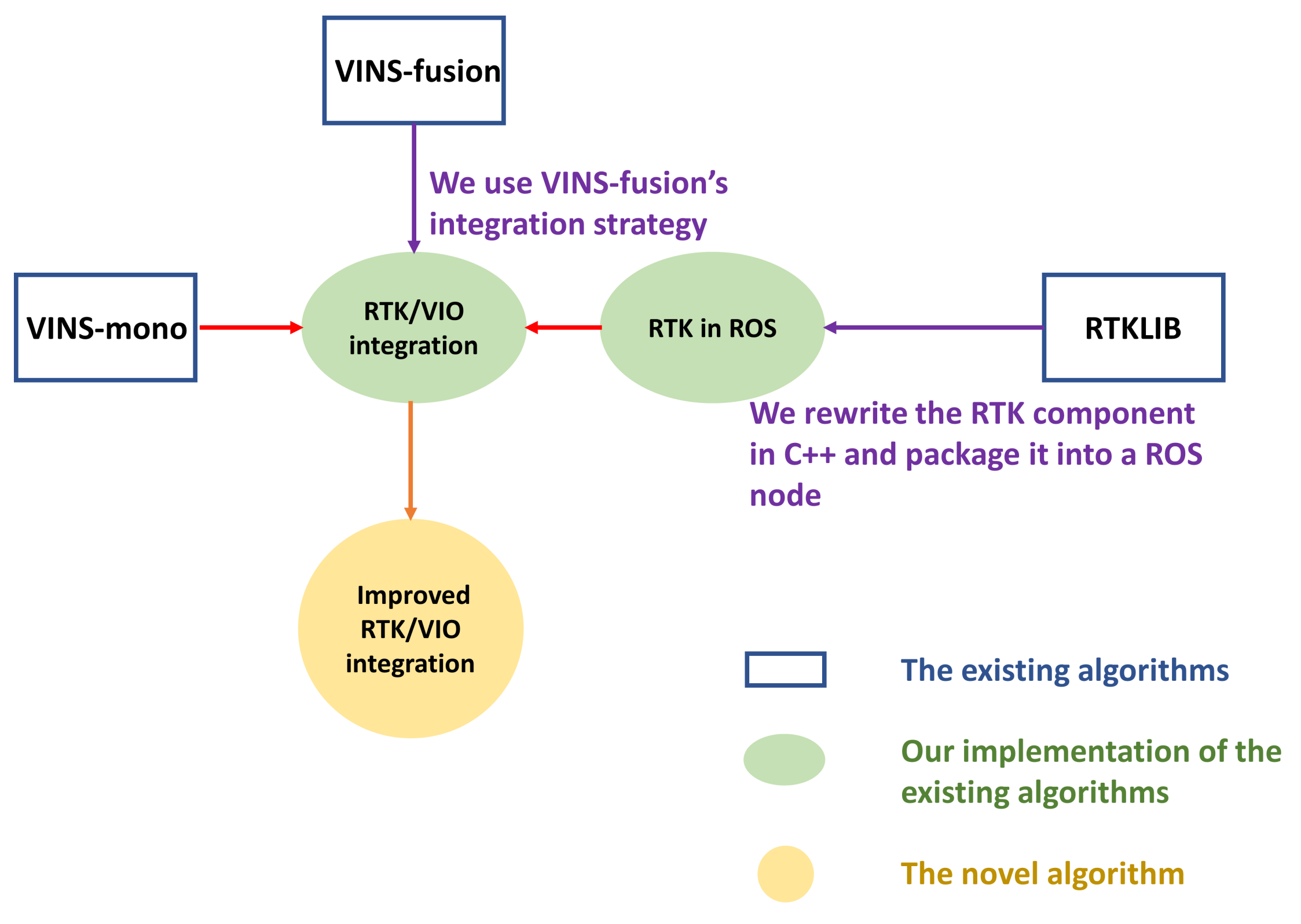
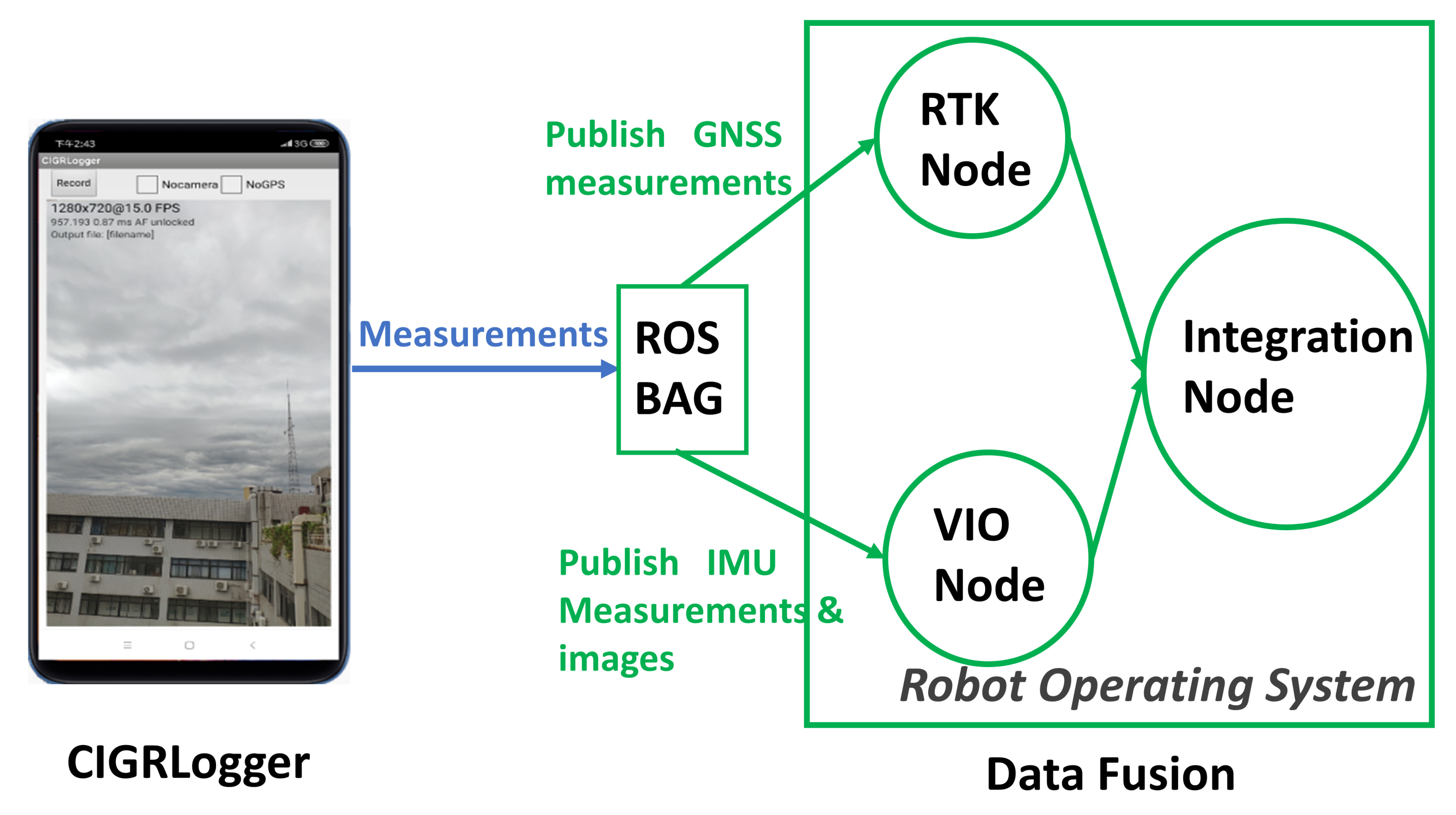
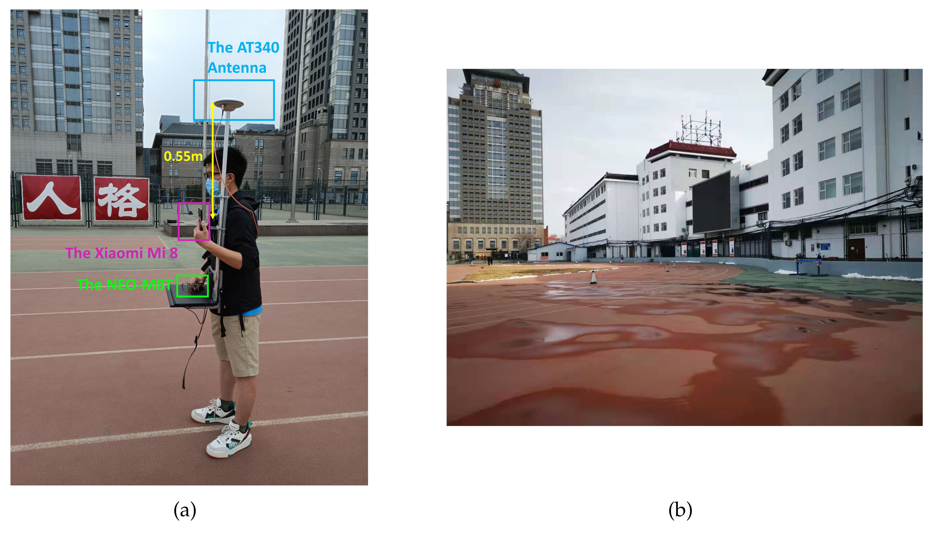
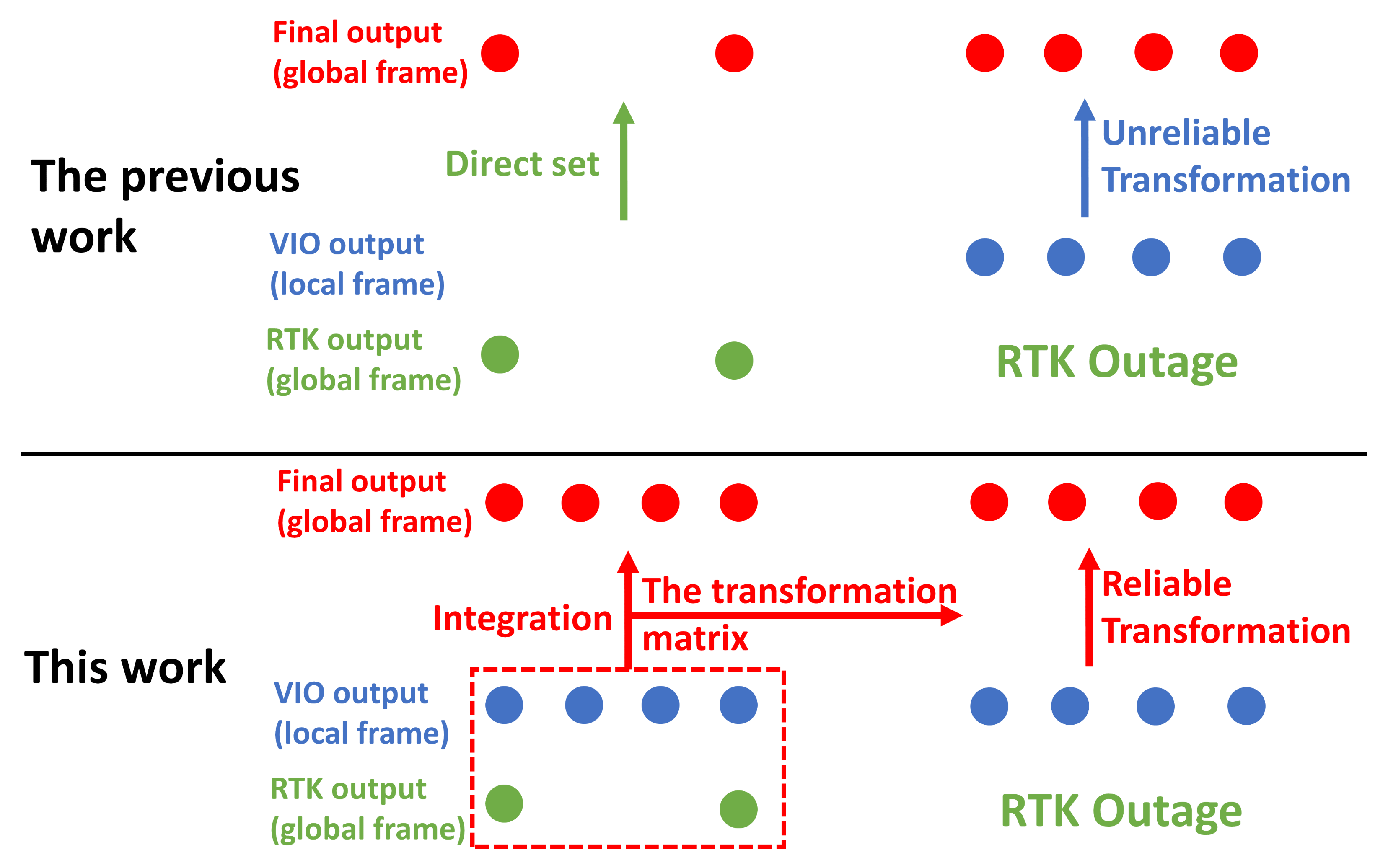
(1) We demonstrate the feasibility of integrating RTK and VIO, using smartphones. Our previous work verifies the feasibility of continuous positioning based on RTK and VIO, using smartphones. However, in our previous work, RTK and VIO do not run simultaneously, but alternate to estimate a positioning solution. The position output from RTK does not affect the output from VIO and vice versa [46]. In our previous work, we combined RTK with VIO in a straightforward and unreliable way. In this paper, we choose more reliable and robust strategies to integrate RTK and VIO. First, we upgrade our CIGRLogger to collect BDS measurements to introduce more valid satellites. Then, as many VIO algorithms are coupled with ROS, we design a Python script to convert the images, IMU measurements, and GNSS measurements into a ROS bag. A ROS bag is a file that stores messages for ROS. Each kind of message has a unique topic. ROS nodes can subscribe to different topics to obtain the data they require. Following that, RTKLIB is a sophisticated system that consists of many algorithms and functions. The algorithm is implemented in ANSI C. We follow RTKLIB’s principle to implement the RTK function in C++ and package these codes into a ROS node. This RTK node subscribes to the topics in the ROS bag created by our Python script and publishes the RTK positioning results to other nodes. This RTK node can be directly integrated into other ROS algorithms. Finally, we adopt the integration strategy of VINS-fusion [35] and integrate our RTK node with VINS-mono [27]. Another node based on optimization is introduced to accomplish the integration. 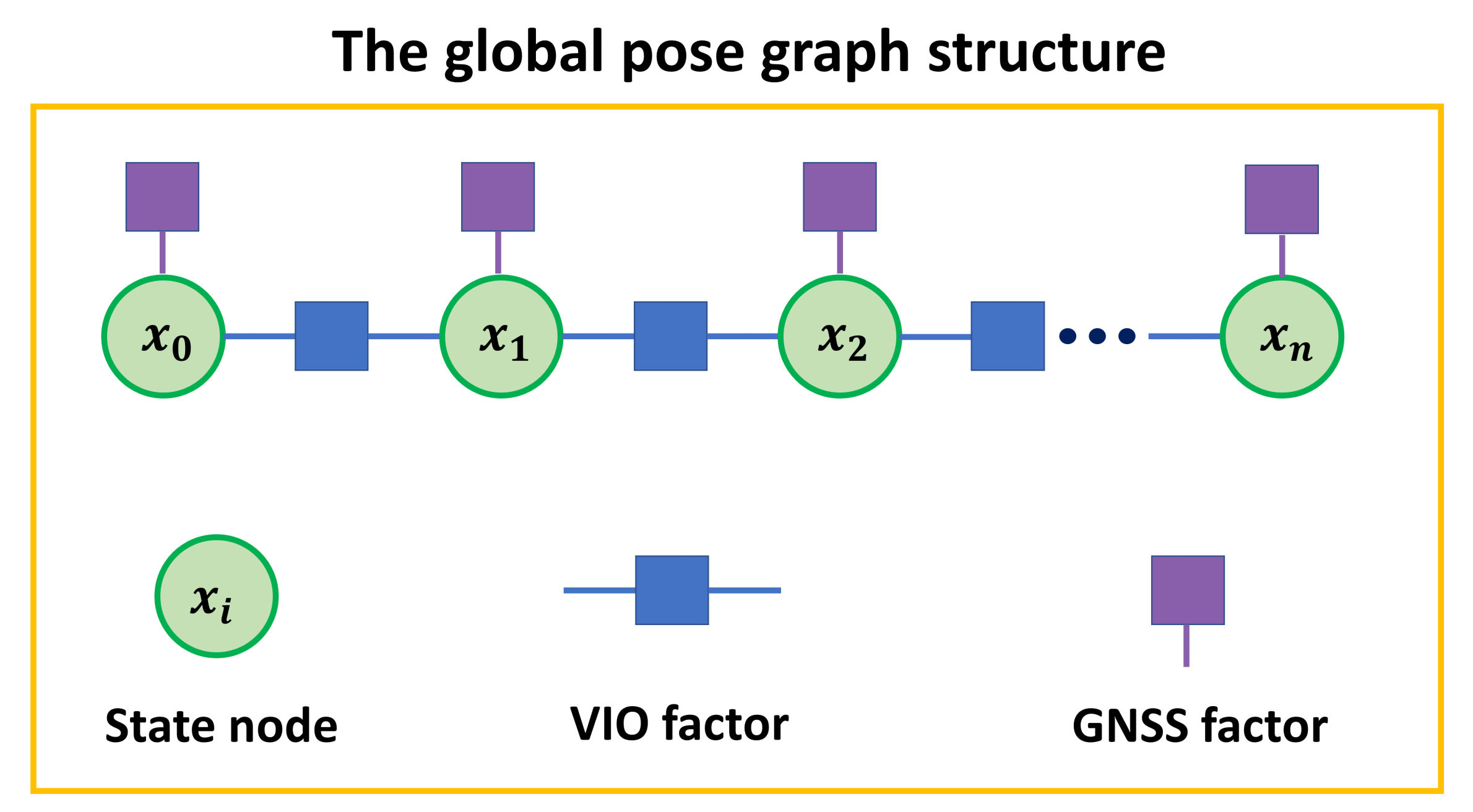The details of the optimization are explained in Section 2.3. The experiments demonstrate that the integration of both approaches combines RTK and VIO’s advantages and can provide accurate continuous positioning results with a smartphone in urban areas.

(2) We provide valuable research tools. As shown in Table 2, many researchers work on the GNSS/INS/VO fusion algorithm based on the bulky and complex specialized devices. We open source our codes on GitHub to facilitate the researchers who lack the resources to build a specialized suite for RTK/VIO integration research. The researchers can collect measurements using an Android smartphone with CIGRLogger. They do not need to implement RTK nodes themselves, which saves time and effort. The academics can concentrate on integration algorithms without spending too much effort on data acquisition, data transformation, and RTK algorithm implementation.

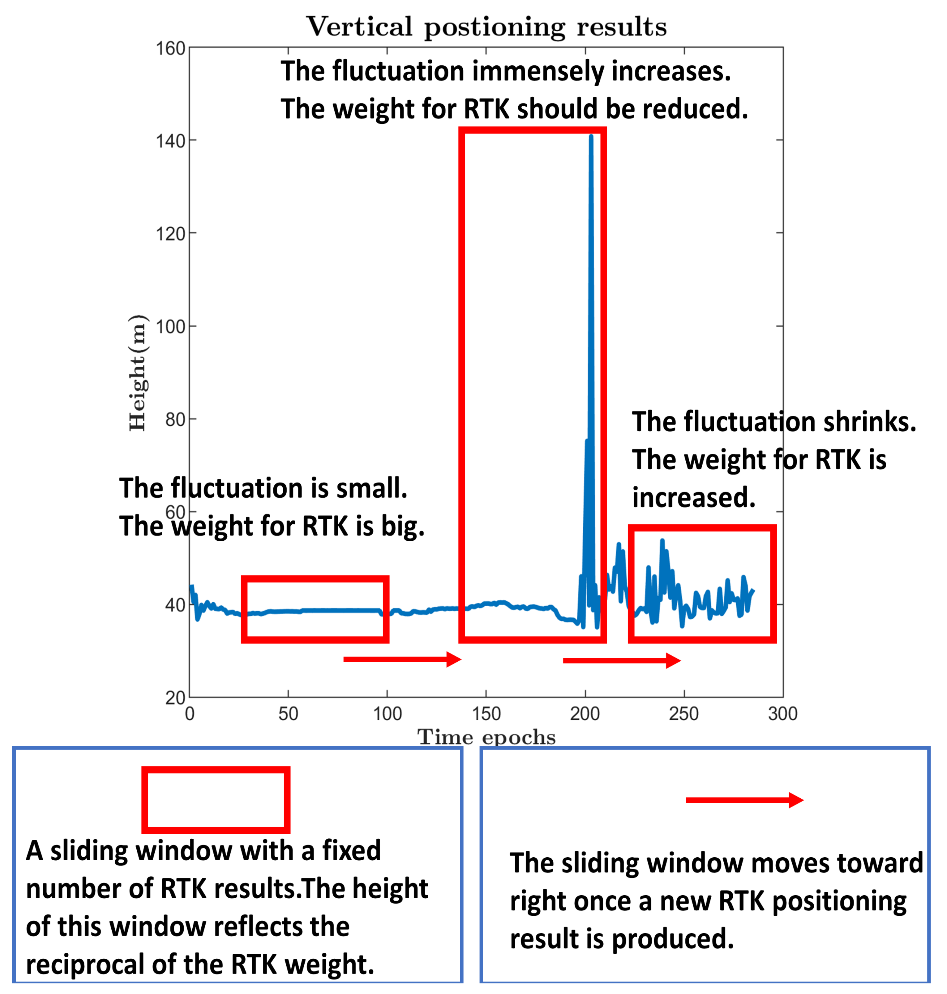
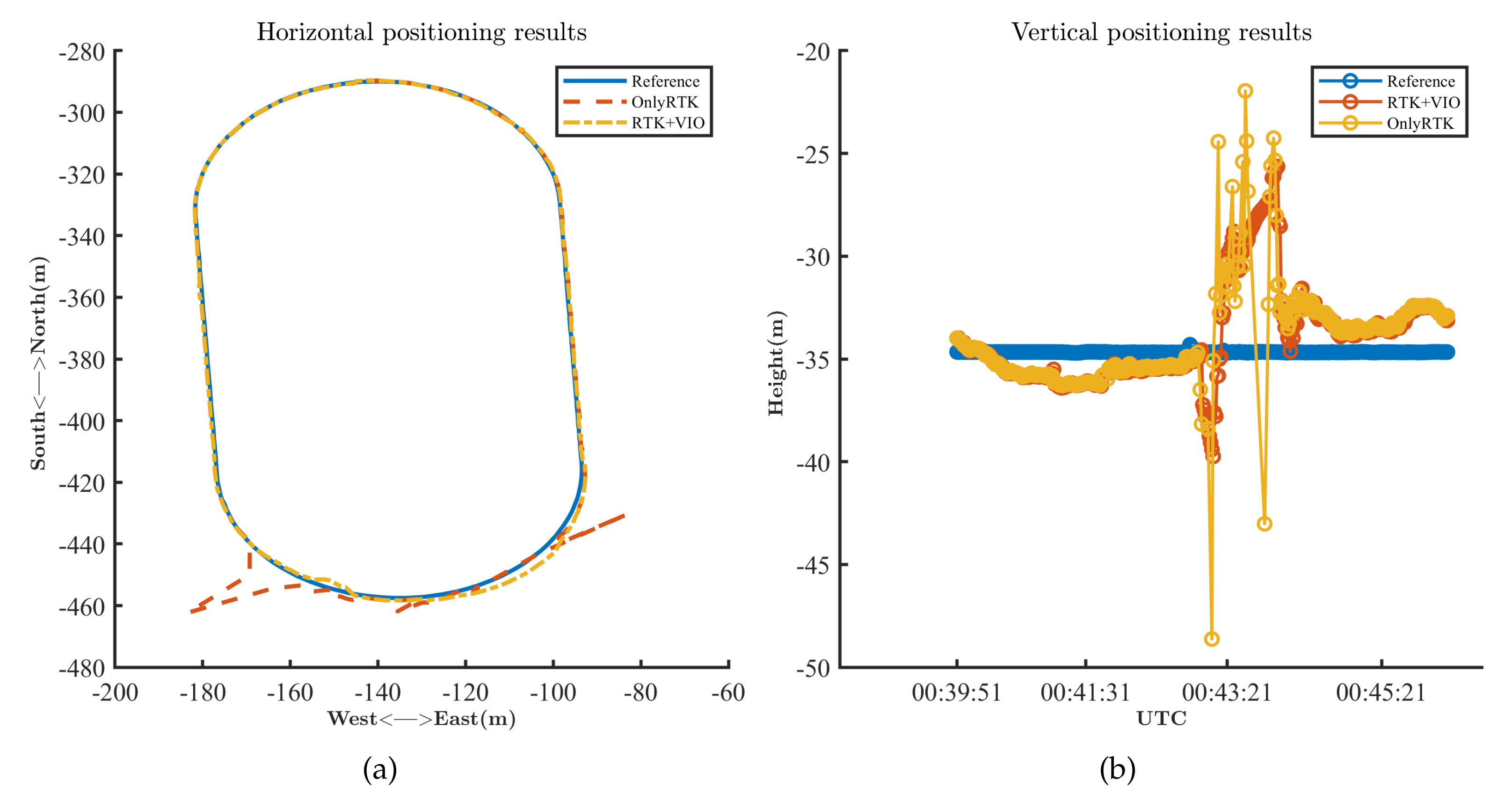
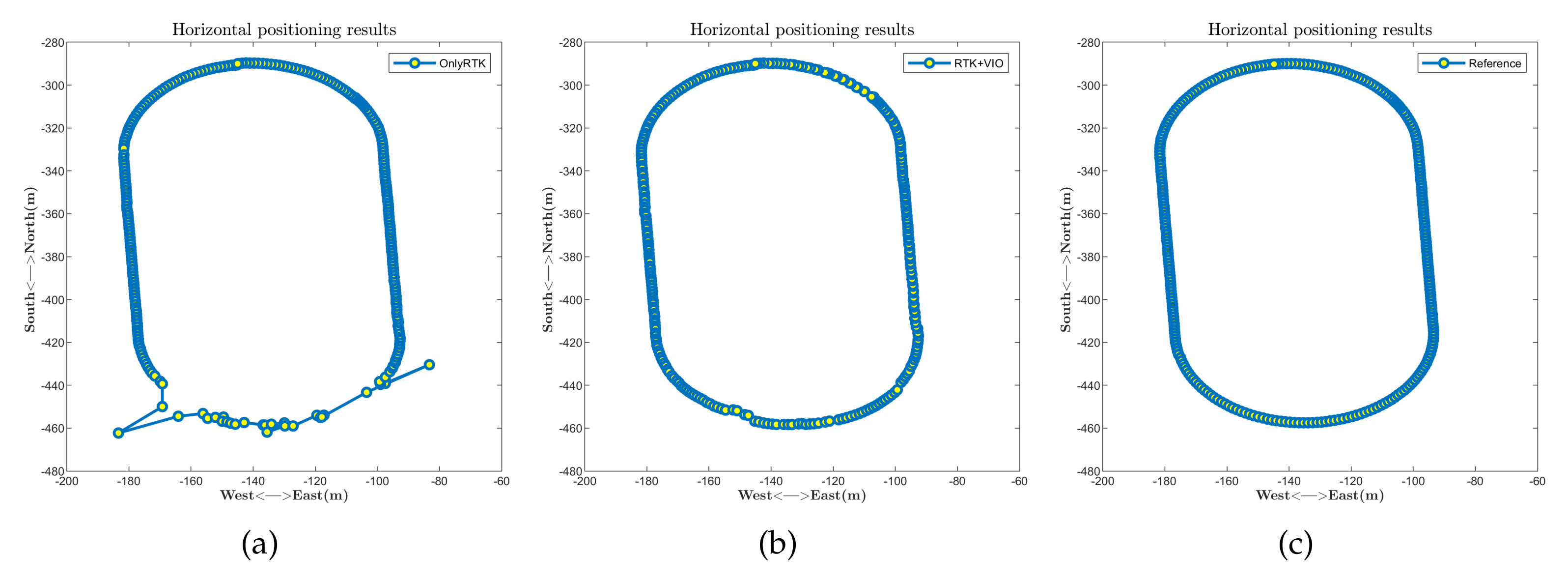
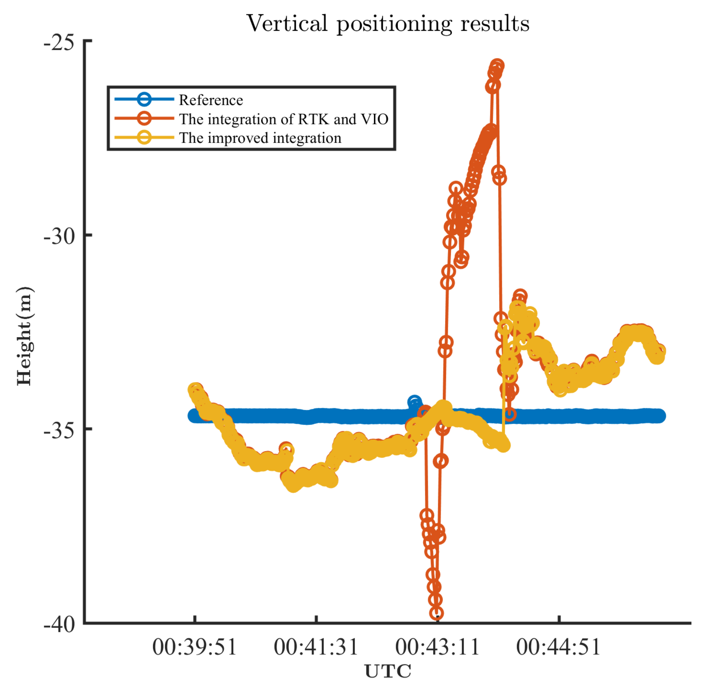
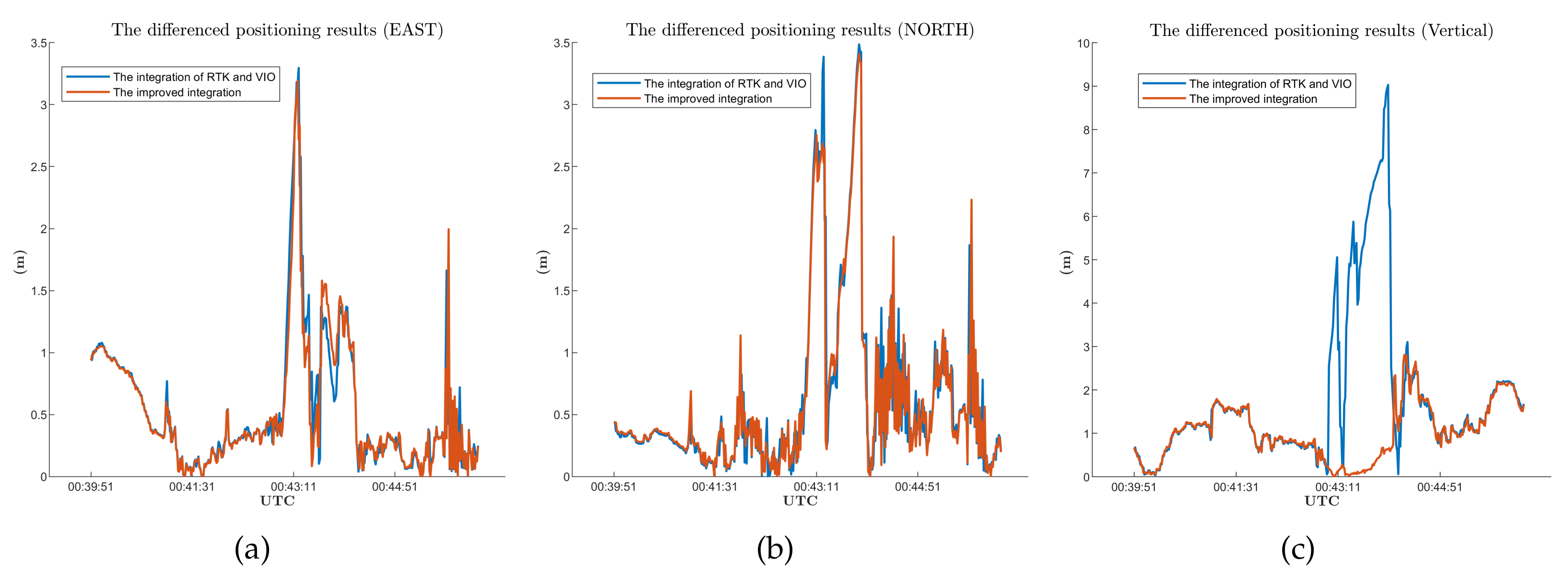
(3) We improve the integration strategy for smartphones. The positioning results provided by RTK with a smartphone can fluctuate immensely. Due to the geometric distribution of satellites, these fluctuations are more pronounced in vertical positioning. We design a sliding window strategy and calculate the vertical positioning fluctuations in the window. The result is treated as a criterion to adjust the weight for RTK in integration. This improvement decreases the deviation in altitude positioning results when compared to the VINS-fusion integration strategy.

As our work involves several existing algorithms, we use Figure 1 to depict the relationship between the existing algorithms and our work.

The remainder of the paper is structured as follows: Section 2 discusses the RTK algorithm, the framework of VINS-mono, the integration strategy of VINS-fusion, the improvement of integration, and some specifics regarding our tools and devices. Next, Section 3 introduces the results of the experiments. Finally, Section 4 summarizes the conclusions and future work.

2. Materials and Methods

This section introduces the principles of the existing techniques utilized by us and our novel algorithm. The existing techniques include RTK in Section 2.1, VINS-mono in Section 2.2, and VINS-fusion in Section 2.3. Our proposed algorithm is introduced in Section 2.4. We introduce the details about our experiments in Section 2.5. A comparison between this work and our previous work is presented in Section 2.6.

In this section, we use t to denote the time. We use $\Delta t$ to denote the time interval between two adjacent sampling epochs. We use a notation that is followed by $\left(t\right)$ to denote a variable that changes over time.

2.1. Implementation of RTK

This section introduces the RTKLIB principle [9,54]. We implement our RTK node in C++ following this principle. The current version of our RTK node has no algorithmic innovations when compared to RTKLIB. We use “$\mathrm{G}$” as a descriptive term for GPS and use “$\mathrm{B}$” as a descriptive term for BDS.

2.1.1. The Single Difference and the Double Difference

RTK is a differential positioning technique involving a single difference (SD) and a double difference (DD). The SD and DD techniques can mitigate the influence of biases because the measurements of the user and those of the reference station are correlated. Figure 2a depicts the geometry of two satellites and two receivers. Figure 2b explains how to calculate the SD and DD measurements [55].

In Figure 2a, $\mathit{o}\left(t\right)$ with the specific superscript and subscript is the unit line-of-sight (LOS) vector from a receiver to a satellite. In Figure 2, $\rho \left(t\right)$ with the specific superscript and the specific subscript denotes the pseudo-range between the corresponding receiver and the corresponding satellite. The carrier phase measurements are denoted by $\varphi \left(t\right)$ with different superscripts and subscripts. The pseudo-range and the carrier phase are formulated as shown in Equations (1) and (2):

$$\rho \left(t\right)=r\left(t\right)+{\tau }_{\mathrm{iono}}\left(t\right)+{\tau }_{\mathrm{tropo}}\left(t\right)+c(\delta {}_{\mathrm{rec}}\left(t\right)-\delta {}_{\mathrm{sat}}\left(t\right))+{\omega }_{\rho }\left(t\right),$$

(1)

$$\varphi \left(t\right)={\lambda }^{-1}[r\left(t\right)-{\tau }_{\mathrm{iono}}\left(t\right)+{\tau }_{\mathrm{tropo}}\left(t\right)+c(\delta {}_{\mathrm{rec}}\left(t\right)-\delta {}_{\mathrm{sat}}\left(t\right))]+N+{\omega }_{\varphi }\left(t\right).$$

(2)

In Equations (1) and (2), $r\left(t\right)$ denotes the geometric distance between the receiver and the satellite in meters; $\lambda$ and N represent the wavelength and the integer ambiguity, respectively; $\omega \left(t\right)$ with different subscripts are the measurement noise and unmodeled error in the pseudo-range and carrier phase, respectively; ${\tau }_{\mathrm{iono}}\left(t\right)$ and ${\tau }_{\mathrm{tropo}}\left(t\right)$ refer to the ionospheric delay and the tropospheric delay, respectively; $\delta {}_{\mathrm{rec}}\left(t\right)$ and $\delta {}_{\mathrm{sat}}\left(t\right)$ denote the receiver clock bias and the satellite clock bias, respectively; and c stands for the speed of light. The carrier phase measurements are more precise than the pseudo-range measurements. The phase tracking loop uses a numerically controlled oscillator (NCO) to generate a local signal with the same frequency and phase as the received signal. The loop utilizes a phase discriminator and a filter to compute the feedback to the NCO. The discriminator cannot distinguish between one cycle and another and thus, converges to the nearest cycle. The NCO can only match the phase of the local and received signals within one cycle. As a result, the carrier phases are ambiguous by an unknown integer number of wavelengths, which is denoted by N. RTK utilizes the SD and DD measurements to eliminate the influences of the clock biases and the delays and employs the AR technique to calculate the ambiguities for the carrier phases.

In Figure 2b, the SD pseudo-range and the SD carrier phase are denoted by $\Delta \rho \left(t\right)$ and $\Delta \varphi \left(t\right)$. SD measurements eliminate the influence introduced by the satellite clock bias. When used in short-baseline RTK, the SD technique can eliminate most ionospheric delays and tropospheric delays. $\nabla \Delta \rho \left(t\right)$ and $\nabla \Delta \varphi \left(t\right)$ refer to the DD pseudo-range and the DD carrier phase, respectively. DD measurements have the advantage of removing the influence of the receiver clock bias. In short-baseline RTK, the DD pseudo-range and DD carrier phase are represented in meters as follows:

$$\nabla \Delta \rho \left(t\right)=\nabla \Delta r\left(t\right)+\nabla \Delta {\omega }_{\rho }\left(t\right),$$

(3)

$$\lambda \nabla \Delta \varphi \left(t\right)=\nabla \Delta r\left(t\right)+\nabla \Delta N\left(t\right)+\nabla \Delta {\omega }_{\varphi }\left(t\right),$$

(4)

where $\nabla \Delta (·)$ denotes the DD operator. The state vector of the RTK Kalman filter is composed by the integer ambiguities, and the measurement vector is composed by the DD pseudo-ranges and DD carrier phases. Each GNSS system has its own time reference. A time offset exists between GPS and BDS, and the clock biases of different systems are different. Admittedly, a GNSS system can broadcast the ephemeris that includes the information of the satellite clock bias. However, the satellite clock bias calculated in this way is not accurate enough. The SD and DD techniques are introduced to eliminate the influence of the clock bias. If we choose only one reference satellite for GPS and BDS, we should model the clock bias between two systems and estimate it, which can degrade the positioning accuracy. In this paper, we only make DD between satellites of the same systems to eliminate the clock biases more completely.

2.1.2. RTK’s Kalman Filter

RTKLIB is built on an EKF that consists of two steps: prediction and update. The EKF provides floating ambiguity solutions. The lambda algorithm [56] is then used to search for integer ambiguity solutions. This section discusses the EKF in detail for GPS/BDS single-frequency RTK. The state vector ${\mathbf{\chi }}_{{}_{\mathrm{RTK}}}\left(t\right)$, in general, contains the SD phase ambiguities and the position. We can expand the state vector and use the velocity and acceleration to smoothen the position fluctuations. If we extend the state vector and consider two constellations, the state vector can be represented as Equation (5):

$${\mathbf{\chi }}_{{}_{\mathrm{RTK}}}\left(t\right)={({\mathit{d}}_{\mathrm{u}}{\left(t\right)}^{\mathrm{T}},{\mathit{v}}_{\mathrm{u}}{\left(t\right)}^{\mathrm{T}},{\mathit{a}}_{\mathrm{u}}{\left(t\right)}^{\mathrm{T}},{\mathit{e}}_{{}_{\mathrm{G}}}{\left(t\right)}^{\mathrm{T}},{\mathit{e}}_{{}_{\mathrm{B}}}{\left(t\right)}^{\mathrm{T}})}^{\mathrm{T}}.$$

(5)

In Equation (5), ${\mathit{d}}_{\mathrm{u}}\left(t\right)$ refers to the user’s position; ${\mathit{v}}_{\mathrm{u}}\left(t\right)$ refers to the user’s velocity; ${\mathit{a}}_{\mathrm{u}}\left(t\right)$ refers to the user’s acceleration; ${\mathit{e}}_{{}_{\mathrm{G}}}\left(t\right)$ stands for the SD phase ambiguities of GPS satellites, and ${\mathit{e}}_{{}_{\mathrm{B}}}\left(t\right)$ stands for the SD phase ambiguities of BDS satellites.

We define the measurement vector $\mathit{y}\left(t\right)$ as Equation (6):

$$\mathit{y}\left(t\right)={(\nabla \Delta {\mathbf{\varphi }}_{{}_{\mathrm{G}}}{\left(t\right)}^{\mathrm{T}},\nabla \Delta {\mathbf{\rho }}_{{}_{\mathrm{G}}}{\left(t\right)}^{\mathrm{T}},\nabla \Delta {\mathbf{\varphi }}_{{}_{\mathrm{B}}}{\left(t\right)}^{\mathrm{T}},\nabla \Delta {\mathbf{\rho }}_{{}_{\mathrm{B}}}{\left(t\right)}^{\mathrm{T}})}^{\mathrm{T}}.$$

(6)

In Equation (6), $\nabla \Delta {\mathbf{\varphi }}_{{}_{\mathrm{G}}}\left(t\right)$ and $\nabla \Delta {\mathbf{\varphi }}_{{}_{\mathrm{B}}}\left(t\right)$ represent the DD carrier phase vectors of GPS satellites and BDS satellites, respectively. $\nabla \Delta {\mathbf{\rho }}_{{}_{\mathrm{G}}}\left(t\right)$ and $\nabla \Delta {\mathbf{\rho }}_{{}_{\mathrm{B}}}\left(t\right)$ refer to the DD pseudo-range vectors of GPS satellites and BDS satellites, respectively.

We use the variables $m_{{}_{\mathrm{G}}}$ and $m_{{}_{\mathrm{B}}}$ to represent the numbers of visible GPS satellites and visible BDS satellites, respectively. $m_{{}_{\mathrm{G}}}$ and $m_{{}_{\mathrm{B}}}$ are not necessarily equal. We define the state transition matrix as follows:

$$\mathit{F}\left(t\right)=\left[\begin{array}{ccccc}{\mathit{I}}_{3\times 3}& {\mathit{I}}_{3\times 3}·\Delta t& {\mathit{I}}_{3\times 3}·\frac{{(\Delta t)}^2}{2}& {\mathit{O}}_{3\times m_{{}_{\mathrm{G}}}}& {\mathit{O}}_{3\times m_{{}_{\mathrm{B}}}}\\ {\mathit{O}}_{3\times 3}& {\mathit{I}}_{3\times 3}& {\mathit{I}}_{3\times 3}·\Delta t& {\mathit{O}}_{3\times m_{{}_{\mathrm{G}}}}& {\mathit{O}}_{3\times m_{{}_{\mathrm{B}}}}\\ {\mathit{O}}_{3\times 3}& {\mathit{O}}_{3\times 3}& {\mathit{I}}_{3\times 3}& {\mathit{O}}_{3\times m_{{}_{\mathrm{G}}}}& {\mathit{O}}_{3\times m_{{}_{\mathrm{B}}}}\\ {\mathit{O}}_{m_{{}_{\mathrm{G}}}\times 3}& {\mathit{O}}_{m_{{}_{\mathrm{G}}}\times 3}& {\mathit{O}}_{m_{{}_{\mathrm{G}}}\times 3}& {\mathit{I}}_{m_{{}_{\mathrm{G}}}\times m_{{}_{\mathrm{G}}}}& {\mathit{O}}_{m_{{}_{\mathrm{G}}}\times m_{{}_{\mathrm{B}}}}\\ {\mathit{O}}_{m_{{}_{\mathrm{B}}}\times 3}& {\mathit{O}}_{m_{{}_{\mathrm{B}}}\times 3}& {\mathit{O}}_{m_{{}_{\mathrm{B}}}\times 3}& {\mathit{O}}_{m_{{}_{\mathrm{B}}}\times m_{{}_{\mathrm{G}}}}& {\mathit{I}}_{m_{{}_{\mathrm{B}}}\times m_{{}_{\mathrm{B}}}}\end{array}\right].$$

(7)

In Equation (7), $\mathit{I}$ with different subscripts denotes identity matrices of different dimensions; $\mathit{O}$ with various subscripts denotes zero matrices of varying dimensions. $\mathit{F}\left(t\right)$ is derived from fundamental kinematics theory and the fact that the carrier phase ambiguity is constant during uninterrupted tracking of a satellite signal. We use $\mathit{Q}\left(t\right)$ to denote the covariance matrix of the process noise as shown in Equations (8)–(10):

$$\mathit{Q}\left(t\right)=\left[\begin{array}{ccccc}{\mathit{O}}_{3\times 3}& {\mathit{O}}_{3\times 3}& {\mathit{O}}_{3\times 3}& {\mathit{O}}_{3\times m_{{}_{\mathrm{G}}}}& {\mathit{O}}_{3\times m_{{}_{\mathrm{B}}}}\\ {\mathit{O}}_{3\times 3}& {\mathit{Q}}_1\left(t\right)& {\mathit{O}}_{3\times 3}& {\mathit{O}}_{3\times m_{{}_{\mathrm{G}}}}& {\mathit{O}}_{3\times m_{{}_{\mathrm{B}}}}\\ {{O}}_{3\times 3}& {{O}}_{3\times 3}& {\mathit{O}}_{3\times 3}& {\mathit{O}}_{3\times m_{{}_{\mathrm{G}}}}& {\mathit{O}}_{3\times m_{{}_{\mathrm{B}}}}\\ {\mathit{O}}_{m_{{}_{\mathrm{G}}}\times 3}& {\mathit{O}}_{m_{{}_{\mathrm{G}}}\times 3}& {\mathit{O}}_{m_{{}_{\mathrm{G}}}\times 3}& {\mathit{O}}_{m_{{}_{\mathrm{G}}}\times m_{{}_{\mathrm{G}}}}& {\mathit{O}}_{m_{{}_{\mathrm{G}}}\times m_{{}_{\mathrm{B}}}}\\ {\mathit{O}}_{m_{{}_{\mathrm{B}}}\times 3}& {\mathit{O}}_{m_{{}_{\mathrm{B}}}\times 3}& {\mathit{O}}_{m_{{}_{\mathrm{B}}}\times 3}& {\mathit{O}}_{m_{{}_{\mathrm{B}}}\times m_{{}_{\mathrm{G}}}}& {\mathit{O}}_{m_{{}_{\mathrm{B}}}\times m_{{}_{\mathrm{B}}}}\end{array}\right],$$

(8)

$${\mathit{Q}}_1\left(t\right)={\mathit{R}}_{{}_{\mathrm{ENU}}}^{{}^{\mathrm{ECEF}}}\left(t\right){\mathit{Q}}_2\left(t\right){\mathit{R}}_{{}_{\mathrm{ENU}}}^{{}^{\mathrm{ECEF}}}{\left(t\right)}^{\mathrm{T}},$$

(9)

$${\mathit{Q}}_2\left(t\right)=\left[\begin{array}{ccc}{\sigma }_{ve}^2\Delta t& 0& 0\\ 0& {\sigma }_{vn}^2\Delta t& 0\\ 0& 0& {\sigma }_{vu}^2\Delta t\end{array}\right].$$

(10)

In Equation (9), ${\mathit{R}}_{{}_{\mathrm{ENU}}}^{{}^{\mathrm{ECEF}}}\left(t\right)$ refers to the coordinates rotation matrix from the east-north-up (ENU) coordinate to the Earth-centered and Earth-fixed (ECEF) coordinate. In Equation (10), ${\sigma }_{ve}$, ${\sigma }_{vn}$, and ${\sigma }_{vu}$ are the standard deviations of east, north, and up components of the user’s velocity.

We use $E\left(t\right)$ with different superscripts to denote different satellites’ SD phase ambiguity state variable. The relationship between $\mathbf{e}\left(t\right)$ in the state vector in Equation (5) and $E\left(t\right)$ is shown in Equation (11):

$$\begin{array}{cc}\hfill {\mathit{e}}_{{}_{\mathrm{G}}}{\left(t\right)}^{\mathrm{T}}& =\left[\begin{array}{cccccc}{E}^{S_{{\mathrm{G}}_1}}\left(t\right),& E^{S_{{\mathrm{G}}_2}}\left(t\right),& \dots & E^{S_{{\mathrm{G}}_{k_1}}}\left(t\right),& \dots & E^{S_{{\mathrm{G}}_{m_{\mathrm{G}}}}}\left(t\right)\end{array}\right],\hfill \\ \hfill {\mathit{e}}_{{}_{\mathrm{B}}}{\left(t\right)}^{\mathrm{T}}& =\left[\begin{array}{cccccc}{E}^{S_{{\mathrm{B}}_1}}\left(t\right),& E^{S_{{\mathrm{B}}_2}}\left(t\right),& \dots & E^{S_{{\mathrm{B}}_{k_2}}}\left(t\right),& \dots & E^{S_{{\mathrm{B}}_{m_{\mathrm{B}}}}}\left(t\right)\end{array}\right].\hfill \end{array}$$

(11)

In Equation (11), $k_1$ and $k_2$ refer to the indices of GPS satellites and BDS satellites, respectively. $S_{{\mathrm{G}}_{k_1}}$ denotes the $k_1$th GPS satellite, while $S_{{\mathrm{B}}_{k_2}}$ denotes the $k_2$th BDS satellite.

We use $\nabla \Delta r^{S_{{\mathrm{G}}_1},S_{{\mathrm{G}}_{k_1}}}\left(t\right)$ to denote the DD geometric range between the 1st GPS satellite and the $k_1$th GPS satellite. We use $\nabla \Delta r^{S_{{\mathrm{B}}_1},S_{{\mathrm{B}}_{k_2}}}\left(t\right)$ to denote the DD geometric range between the 1st BDS satellite and the $k_2$th BDS satellite. $\nabla \Delta r^{S_{{\mathrm{G}}_1},S_{{\mathrm{G}}_{k_1}}}\left(t\right)$ and $\nabla \Delta r^{S_{{\mathrm{B}}_1},S_{{\mathrm{B}}_{k_2}}}\left(t\right)$ can be calculated using the user’s position in the state vector in Equation (5) and the satellites’ position as shown in Equation (12):

$$\begin{array}{cc}\hfill \nabla \Delta r^{S_{{\mathrm{G}}_1},S_{{\mathrm{G}}_{k_1}}}\left(t\right)& =|{\mathit{d}}_{S_{{\mathrm{G}}_1}}\left(t\right)-{\mathit{d}}_{\mathrm{u}}\left(t\right)|-|{\mathit{d}}_{S_{{\mathrm{G}}_1}}\left(t\right)-{\mathit{d}}_{\mathrm{ref}}|-(|{\mathit{d}}_{S_{{\mathrm{G}}_{{\mathrm{k}}_1}}}\left(t\right)-{\mathit{d}}_{\mathrm{u}}\left(t\right)|-|{\mathit{d}}_{S_{{\mathrm{G}}_{{\mathrm{k}}_1}}}\left(t\right)-{\mathit{d}}_{\mathrm{ref}}\left|\right),\hfill \\ \hfill \nabla \Delta r^{S_{{\mathrm{B}}_1},S_{{\mathrm{B}}_{k_2}}}\left(t\right)& =|{\mathit{d}}_{S_{{\mathrm{B}}_1}}\left(t\right)-{\mathit{d}}_{\mathrm{u}}\left(t\right)|-|{\mathit{d}}_{S_{{\mathrm{B}}_1}}\left(t\right)-{\mathit{d}}_{\mathrm{ref}}|-(|{\mathit{d}}_{S_{{\mathrm{B}}_{{\mathrm{k}}_2}}}\left(t\right)-{\mathit{d}}_{\mathrm{u}}\left(t\right)|-|{\mathit{d}}_{S_{{\mathrm{B}}_{{\mathrm{k}}_2}}}\left(t\right)-{\mathit{d}}_{\mathrm{ref}}\left|\right).\hfill \end{array}$$

(12)

In Equation (12), ${\mathit{d}}_{S_{{\mathrm{G}}_{{\mathrm{k}}_1}}}\left(t\right)$ denotes the position of the $k_1$th GPS satellite, and ${\mathit{d}}_{S_{{\mathrm{B}}_{{\mathrm{k}}_2}}}\left(t\right)$ refers to the position of the $k_2$th BDS satellite. The position of a satellite is calculated using the ephemeris broadcast by the satellite. ${\mathit{d}}_{\mathrm{ref}}$ is the position of the reference station.

We use $\mathit{h}\left({\mathbf{\chi }}_{{}_{\mathrm{RTK}}}\left(t\right)\right)$ to refer to the the measurement function for the update step. The measurement function consists of four sub-functions as shown in Equation (13):

$$\mathit{h}\left({\mathbf{\chi }}_{{}_{\mathrm{RTK}}}\left(t\right)\right)={({\mathit{h}}_{{\mathsf{\Phi }}_{{}_{\mathrm{G}}}}{({\mathit{d}}_{\mathrm{u}}\left(t\right),{\mathit{e}}_{{}_{\mathrm{G}}}\left(t\right))}^{\mathrm{T}},{\mathit{h}}_{{\rho }_{{}_{\mathrm{G}}}}{\left({\mathit{d}}_{\mathrm{u}}\left(t\right)\right)}^{\mathrm{T}},{\mathit{h}}_{{\mathsf{\Phi }}_{{}_{\mathrm{B}}}}{({\mathit{d}}_{\mathrm{u}}\left(t\right),{\mathit{e}}_{{}_{\mathrm{B}}}\left(t\right))}^{\mathrm{T}},{\mathit{h}}_{{\rho }_{{}_{\mathrm{B}}}}{\left({\mathit{d}}_{\mathrm{u}}\left(t\right)\right)}^{\mathrm{T}})}^{\mathrm{T}},$$

(13)

where:

$$\begin{array}{cc}\hfill {\mathit{h}}_{{\mathsf{\Phi }}_{{}_{\mathrm{G}}}}({\mathit{d}}_{\mathrm{u}}\left(t\right),{\mathit{e}}_{{}_{\mathrm{G}}}\left(t\right))& =\left[\begin{array}{c}\nabla \Delta r^{S_{{\mathrm{G}}_1},S_{{\mathrm{G}}_2}}\left(t\right)+{\lambda }_{{}_{\mathrm{G}}}(E^{S_{{\mathrm{G}}_1}}\left(t\right)-E^{S_{{\mathrm{G}}_2}}\left(t\right))\\ \nabla \Delta r^{S_{{\mathrm{G}}_1},S_{{\mathrm{G}}_3}}\left(t\right)+{\lambda }_{{}_{\mathrm{G}}}(E^{S_{{\mathrm{G}}_1}}\left(t\right)-E^{S_{{\mathrm{G}}_3}}\left(t\right))\\ ⋮\\ \nabla \Delta r^{S_{{\mathrm{G}}_1},S_{{\mathrm{G}}_{k_1}}}\left(t\right)+{\lambda }_{{}_{\mathrm{G}}}(E^{S_{{\mathrm{G}}_1}}\left(t\right)-E^{S_{{\mathrm{G}}_{k_1}}}\left(t\right))\\ ⋮\\ \nabla \Delta r^{S_{{\mathrm{G}}_1},S_{{\mathrm{G}}_{m_{\mathrm{G}}}}}\left(t\right)+{\lambda }_{{}_{\mathrm{G}}}(E^{S_{{\mathrm{G}}_1}}\left(t\right)-E^{S_{{\mathrm{G}}_{m_{\mathrm{G}}}}}\left(t\right))\end{array}\right],\hfill \\ \hfill {\mathit{h}}_{{\mathsf{\Phi }}_{{}_{\mathrm{B}}}}({\mathit{d}}_{\mathrm{u}}\left(t\right),{\mathit{e}}_{{}_{\mathrm{B}}}\left(t\right))& =\left[\begin{array}{c}\nabla \Delta r^{S_{{\mathrm{B}}_1},S_{{\mathrm{B}}_2}}\left(t\right)+{\lambda }_{{}_{\mathrm{B}}}(E^{S_{{\mathrm{B}}_1}}\left(t\right)-E^{S_{{\mathrm{B}}_2}}\left(t\right))\\ \nabla \Delta r^{S_{{\mathrm{B}}_1},S_{{\mathrm{B}}_3}}\left(t\right)+{\lambda }_{{}_{\mathrm{B}}}(E^{S_{{\mathrm{B}}_1}}\left(t\right)-E^{S_{{\mathrm{B}}_3}}\left(t\right))\\ ⋮\\ \nabla \Delta r^{S_{{\mathrm{B}}_1},S_{{\mathrm{B}}_{k_2}}}\left(t\right)+{\lambda }_{{}_{\mathrm{B}}}(E^{S_{{\mathrm{B}}_1}}\left(t\right)-E^{S_{{\mathrm{B}}_{k_2}}}\left(t\right))\\ ⋮\\ \nabla \Delta r^{S_{{\mathrm{B}}_1},S_{{\mathrm{B}}_{m_{\mathrm{B}}}}}\left(t\right)+{\lambda }_{{}_{\mathrm{B}}}(E^{S_{{\mathrm{B}}_1}}\left(t\right)-E^{S_{{\mathrm{B}}_{m_{\mathrm{B}}}}}\left(t\right))\end{array}\right],\hfill \end{array}$$

(14)

$$\begin{array}{cc}\hfill {\mathit{h}}_{{\rho }_{{}_{\mathrm{G}}}}\left({\mathit{d}}_{\mathrm{u}}\left(t\right)\right)& =\left[\begin{array}{c}\nabla \Delta r^{S_{{\mathrm{G}}_1},S_{{\mathrm{G}}_2}}\left(t\right)\\ \nabla \Delta r^{S_{{\mathrm{G}}_1},S_{{\mathrm{G}}_3}}\left(t\right)\\ ⋮\\ \nabla \Delta r^{S_{{\mathrm{G}}_1},S_{{\mathrm{G}}_{k_1}}}\left(t\right)\\ ⋮\\ \nabla \Delta r^{S_{{\mathrm{G}}_1},S_{{\mathrm{G}}_{m_{\mathrm{G}}}}}\left(t\right)\end{array}\right],\hfill \\ \hfill {\mathit{h}}_{{\rho }_{{}_{\mathrm{B}}}}\left({\mathit{d}}_{\mathrm{u}}\left(t\right)\right)& =\left[\begin{array}{c}\nabla \Delta r^{S_{{\mathrm{B}}_1},S_{{\mathrm{B}}_2}}\left(t\right)\\ \nabla \Delta r^{S_{{\mathrm{B}}_1},S_{{\mathrm{B}}_3}}\left(t\right)\\ ⋮\\ \nabla \Delta r^{S_{{\mathrm{B}}_1},S_{{\mathrm{B}}_{k_2}}}\left(t\right)\\ ⋮\\ \nabla \Delta r^{S_{{\mathrm{B}}_1},S_{{\mathrm{B}}_{m_{\mathrm{B}}}}}\left(t\right)\end{array}\right].\hfill \end{array}$$

(15)

In Equation (14), ${\lambda }_{{}_{\mathrm{G}}}$ and ${\lambda }_{{}_{\mathrm{B}}}$ are the wavelengths of the GPS L1 signal and BDS B1I signal, respectively.

We define ${\mathit{D}}_{{}_{\mathrm{G}}}$ and ${\mathit{D}}_{{}_{\mathrm{B}}}$ as the SD transition matrices for GPS and BDS as shown in Equations (16) and (17):

$${\mathit{D}}_{{}_{\mathrm{G}}}={\left[\begin{array}{ccccc}1& -1& 0& \cdots & 0\\ 1& 0& -1& \cdots & 0\\ ⋮& ⋮& ⋮& \ddots & ⋮\\ 1& 0& 0& \cdots & -1\end{array}\right]}_{(m_{\mathrm{G}}-1)\times m_{\mathrm{G}}},$$

(16)

$${\mathit{D}}_{{}_{\mathrm{B}}}={\left[\begin{array}{ccccc}1& -1& 0& \cdots & 0\\ 1& 0& -1& \cdots & 0\\ ⋮& ⋮& ⋮& \ddots & ⋮\\ 1& 0& 0& \cdots & -1\end{array}\right]}_{(m_{\mathrm{B}}-1)\times m_{\mathrm{B}}}.$$

(17)

We can define ${\mathit{L}}_{{}_{\mathrm{G}}}\left(t\right)$ and ${\mathit{L}}_{{}_{\mathrm{B}}}\left(t\right)$ as matrices comprised of LOS vectors for different constellations as shown in Equations (18) and (19):

$${\mathit{L}}_{{}_{\mathrm{G}}}\left(t\right)={\left[\begin{array}{c}{\mathit{o}}_{{}_{S_{{\mathrm{G}}_1}}}{\left(t\right)}^{\mathrm{T}}\\ {\mathit{o}}_{{}_{S_{{\mathrm{G}}_2}}}{\left(t\right)}^{\mathrm{T}}\\ ⋮\\ {\mathit{o}}_{{}_{S_{{\mathrm{G}}_{{\mathrm{k}}_1}}}}{\left(t\right)}^{\mathrm{T}}\\ ⋮\\ {\mathit{o}}_{{}_{S_{{\mathrm{G}}_{{\mathrm{m}}_{\mathrm{G}}}}}}{\left(t\right)}^{\mathrm{T}}\end{array}\right]}_{m_{\mathrm{G}}\times 3},$$

(18)

$${\mathit{L}}_{{}_{\mathrm{B}}}\left(t\right)={\left[\begin{array}{c}{\mathit{o}}_{{}_{S_{{\mathrm{B}}_1}}}{\left(t\right)}^{\mathrm{T}}\\ {\mathit{o}}_{{}_{S_{{\mathrm{B}}_2}}}{\left(t\right)}^{\mathrm{T}}\\ ⋮\\ {\mathit{o}}_{{}_{S_{{\mathrm{B}}_{{\mathrm{k}}_2}}}}{\left(t\right)}^{\mathrm{T}}\\ ⋮\\ {\mathit{o}}_{{}_{S_{{\mathrm{B}}_{{\mathrm{m}}_{\mathrm{B}}}}}}{\left(t\right)}^{\mathrm{T}}\end{array}\right]}_{m_{\mathrm{B}}\times 3}.$$

(19)

Finally, we can define the observation matrix $\mathit{H}\left(t\right)$ as:

$$\mathit{H}\left(t\right)=\left[\begin{array}{cccc}-{\mathit{D}}_{{}_{\mathrm{G}}}{\mathit{L}}_{{}_{\mathrm{G}}}\left(t\right)& {\mathit{O}}_{(m_{{}_{\mathrm{G}}}-1)\times 6}& {\lambda }_{{}_{\mathrm{G}}}·{\mathit{D}}_{{}_{\mathrm{G}}}& {\mathit{O}}_{(m_{{}_{\mathrm{G}}}-1)\times m_{{}_{\mathrm{B}}}}\\ -{\mathit{D}}_{{}_{\mathrm{G}}}{\mathit{L}}_{{}_{\mathrm{G}}}\left(t\right)& {{O}}_{(m_{{}_{\mathrm{G}}}-1)\times 6}& {\mathit{O}}_{(m_{{}_{\mathrm{G}}}-1)\times m_{{}_{\mathrm{G}}}}& {\mathit{O}}_{(m_{{}_{\mathrm{G}}}-1)\times m_{{}_{\mathrm{B}}}}\\ -{\mathit{D}}_{{}_{\mathrm{B}}}{\mathit{L}}_{{}_{\mathrm{B}}}\left(t\right)& {\mathit{O}}_{(m_{{}_{\mathrm{B}}}-1)\times 6}& {\mathit{O}}_{(m_{{}_{\mathrm{B}}}-1)\times m_{{}_{\mathrm{G}}}}& {\lambda }_{{}_{\mathrm{B}}}·{\mathit{D}}_{{}_{\mathrm{B}}}\\ -{\mathit{D}}_{{}_{\mathrm{B}}}{\mathit{L}}_{{}_{\mathrm{B}}}\left(t\right)& {\mathit{O}}_{(m_{{}_{\mathrm{B}}}-1)\times 6}& {\mathit{O}}_{(m_{{}_{\mathrm{B}}}-1)\times m_{{}_{\mathrm{G}}}}& {\mathit{O}}_{(m_{{}_{\mathrm{B}}}-1)\times m_{{}_{\mathrm{B}}}}\end{array}\right].$$

(20)

We use the $\mathit{C}$ to denote the covariance matrix of the observation noise as follows:

$$\mathit{C}=\left[\begin{array}{cccc}{\mathit{D}}_{{}_{\mathrm{G}}}{\mathit{C}}_{{}_{\varphi ,\mathrm{G}}}{{\mathit{D}}_{{}_{\mathrm{G}}}}^{\mathrm{T}}& {\mathit{O}}_{(m_{{}_{\mathrm{G}}}-1)\times (m_{{}_{\mathrm{G}}}-1)}& {\mathit{O}}_{(m_{{}_{\mathrm{G}}}-1)\times (m_{{}_{\mathrm{B}}}-1)}& {\mathit{O}}_{(m_{{}_{\mathrm{G}}}-1)\times (m_{{}_{\mathrm{B}}}-1)}\\ {\mathit{O}}_{(m_{{}_{\mathrm{G}}}-1)\times (m_{{}_{\mathrm{G}}}-1)}& {\mathit{D}}_{{}_{\mathrm{G}}}{\mathit{C}}_{{}_{\rho ,\mathrm{G}}}{{\mathit{D}}_{{}_{\mathrm{G}}}}^{\mathrm{T}}& {\mathit{O}}_{(m_{{}_{\mathrm{G}}}-1)\times (m_{{}_{\mathrm{B}}}-1)}& {\mathit{O}}_{(m_{{}_{\mathrm{G}}}-1)\times (m_{{}_{\mathrm{B}}}-1)}\\ {\mathit{O}}_{(m_{{}_{\mathrm{B}}}-1)\times (m_{{}_{\mathrm{G}}}-1)}& {\mathit{O}}_{(m_{{}_{\mathrm{B}}}-1)\times (m_{{}_{\mathrm{G}}}-1)}& {\mathit{D}}_{{}_{\mathrm{B}}}{\mathit{C}}_{{}_{\varphi ,\mathrm{B}}}{{\mathit{D}}_{{}_{\mathrm{B}}}}^{\mathrm{T}}& {\mathit{O}}_{(m_{{}_{\mathrm{B}}}-1)\times (m_{{}_{\mathrm{B}}}-1)}\\ {\mathit{O}}_{(m_{{}_{\mathrm{B}}}-1)\times (m_{{}_{\mathrm{G}}}-1)}& {\mathit{O}}_{(m_{{}_{\mathrm{B}}}-1)\times (m_{{}_{\mathrm{G}}}-1)}& {\mathit{O}}_{(m_{{}_{\mathrm{B}}}-1)\times (m_{{}_{\mathrm{B}}}-1)}& {\mathit{D}}_{{}_{\mathrm{B}}}{\mathit{C}}_{{}_{\rho ,\mathrm{B}}}{{\mathit{D}}_{{}_{\mathrm{B}}}}^{\mathrm{T}}\end{array}\right],$$

(21)

$$\begin{array}{cc}\hfill {\mathit{C}}_{{}_{\varphi ,\mathrm{G}}}& =diag(2{{\sigma }_{\varphi }^{S_{{\mathrm{G}}_1}}}^2,2{{\sigma }_{\varphi }^{S_{{\mathrm{G}}_2}}}^2,...2{{\sigma }_{\varphi }^{S_{{\mathrm{G}}_{{\mathrm{k}}_1}}}}^2,...2{{\sigma }_{\varphi }^{S_{{\mathrm{G}}_{{\mathrm{m}}_{\mathrm{G}}}}}}^2),\hfill \\ \hfill {\mathit{C}}_{{}_{\rho ,\mathrm{G}}}& =diag(2{{\sigma }_{\rho }^{S_{{\mathrm{G}}_1}}}^2,2{{\sigma }_{\rho }^{S_{{\mathrm{G}}_2}}}^2,...2{{\sigma }_{\rho }^{S_{{\mathrm{G}}_{{\mathrm{k}}_1}}}}^2,...2{{\sigma }_{\rho }^{S_{{\mathrm{G}}_{{\mathrm{m}}_{\mathrm{G}}}}}}^2),\hfill \\ \hfill {\mathit{C}}_{{}_{\varphi ,\mathrm{B}}}& =diag(2{{\sigma }_{\varphi }^{S_{{\mathrm{B}}_1}}}^2,2{{\sigma }_{\varphi }^{S_{{\mathrm{B}}_2}}}^2,...2{{\sigma }_{\varphi }^{S_{{\mathrm{B}}_{{\mathrm{k}}_2}}}}^2,...2{{\sigma }_{\varphi }^{S_{{\mathrm{B}}_{{\mathrm{m}}_{\mathrm{B}}}}}}^2),\hfill \\ \hfill {\mathit{C}}_{{}_{\rho ,\mathrm{B}}}& =diag(2{{\sigma }_{\rho }^{S_{{\mathrm{B}}_1}}}^2,2{{\sigma }_{\rho }^{S_{{\mathrm{B}}_2}}}^2,...2{{\sigma }_{\rho }^{S_{{\mathrm{B}}_{{\mathrm{k}}_2}}}}^2,...2{{\sigma }_{\rho }^{S_{{\mathrm{B}}_{{\mathrm{m}}_{\mathrm{B}}}}}}^2).\hfill \end{array}$$

(22)

In Equation (22), ${\sigma }_{\varphi }$ and ${\sigma }_{\rho }$ denote the standard deviation of the phase measurement error and the pseudo-range measurement error, respectively.

2.2. The Structure of VINS-Mono

This section summarizes the structure of VINS-mono that integrates recent study achievements in the fields of VIO and simultaneous localization and mapping (SLAM). We now give the frame definitions that we use throughout the remainder of the paper. ${(·)}^{\mathrm{w}}$ denotes the world frame, which corresponds to the pose after initialization. ${(·)}^{\mathrm{b}}$ denotes the body frame, which is the same as the IMU frame. ${(·)}^{\mathrm{cam}}$ refers to the camera frame. Figure 3 illustrates the VINS-mono structure [27].

VINS-mono processes measurements from an IMU and a monocular camera. VINS-mono begins with a measurement preprocessing module that preintegrates IMU measurements and extracts and tracks visual features. The system is subsequently initialized, using preprocessed measurements. The initialization module aligns IMU pre-integrals with feature observations to provide initial values of attitude, velocity, IMU bias, and scale for the system. These initial values enter the nonlinear optimization-based VIO that follows. This tightly coupled VIO makes use of a sliding window to reduce computational resources. VINS-mono defines the state vector as follows:

$${\mathbf{\chi }}_{{}_{\mathrm{V}-\mathrm{mono}}}\left(t\right)={\left[\begin{array}{cccccccccc}{\mathit{x}}_1{\left(t\right)}^{\mathrm{T}},& \cdots & {\mathit{x}}_i{\left(t\right)}^{\mathrm{T}},& \cdots {\mathit{x}}_{n_1}{\left(t\right)}^{\mathrm{T}},& {\mathit{p}}_{\mathrm{cam}}^{\mathrm{b}},& {\mathit{q}}_{\mathrm{cam}}^{\mathrm{b}},& s_1\left(t\right),& \cdots & s_j\left(t\right),& \cdots s_{n_2}\left(t\right)\end{array}\right]}^{\mathrm{T}},$$

(23)

$${\mathit{x}}_i\left(t\right)={\left[\begin{array}{ccccc}{\mathit{p}}_{\mathrm{b},i}^{\mathrm{w}}{\left(t\right)}^{\mathrm{T}},& {\mathit{v}}_{\mathrm{b},i}^{\mathrm{w}}{\left(t\right)}^{\mathrm{T}},& {\mathit{q}}_{\mathrm{b},i}^{\mathrm{w}}{\left(t\right)}^{\mathrm{T}},& {\mathbf{ϵ}}_{\mathrm{acc}}{\left(t\right)}^{\mathrm{T}},& {\mathbf{ϵ}}_{\mathrm{gyro}}{\left(t\right)}^{\mathrm{T}}\end{array}\right]}^{\mathrm{T}},i=1,\cdots ,n_1.$$

(24)

In Equations (23) and (24), ${\mathit{p}}_{\mathrm{cam}}^{\mathrm{b}}$ and ${\mathit{q}}_{\mathrm{cam}}^{\mathrm{b}}$ refer to the rotation and translation from the camera frame to the body frame. We use i and j to denote the keyframe index and the feature index, respectively. ${\mathit{x}}_i\left(t\right)$ in Equations (23) and (24) stands for the IMU state vector when the ith frame is captured. ${\mathit{x}}_i\left(t\right)$ includes the position, velocity, orientation of the IMU in the world frame, and IMU biases in the body frame, as Equation (24) shows. $s_j\left(t\right)$ in Equation (23) denotes the inverse distance of the jth feature from the first observation. The variables $n_1$ and $n_2$ in Equations (23) and (24) denote the number of keyframes and features in the sliding window, respectively.

If a frame is treated as a keyframe, the relocalization module will perform loop detection, using the frame’s features. The relocalization module compares this keyframe to all other keyframes in the database to identify a candidate for loop closure. The information associated with this keyframe is imported into the database. Finally, the pose graph optimization module verifies the relocalization results and establishes the feature-level connections between loop closure candidates and the current keyframe. The VIO module mentioned above uses these feature correspondences to eliminate drifts. Relocalization can enhance VIO performance if a user frequently returns to a location he previously passed through. However, an outdoor user can move around a large region without returning to the position he walked through. We can use RTK and other GNSS techniques instead of relocalization to eliminate drift for outdoor users.

2.3. The Integration Strategy of VINS-Fusion

VINS-fusion loosely couples VIO and GNSS, as it transforms the results of VIO and of GNSS to unified factors to construct the optimization problem. The integration of GNSS and VIO is based on a global pose graph. Figure 4 illustrates this global pose graph structure. This pose graph is a nonlinear least-squares problem [32]. In this section, we use ${(·)}^{\mathrm{g}}$ to denote the global frame.

In Figure 4, a state node represents a pose estimation in the global frame. VINS-fusion involves a VIO module and the global optimization. VINS-fusion’s VIO module defines the state vector as Equation (25) shows. The same symbol in Equations (23) and (25) denotes the same variable. VINS-fusion’s VIO does not estimate the extrinsic parameters. VINS-fusion uses the VIO results as measurements to optimize the pose estimation in the global frame. The pose includes the position ${\mathit{p}}_{\mathrm{b}}^{\mathrm{g}}\left(t\right)$ and the orientation ${\mathit{q}}_{\mathrm{b}}^{\mathrm{g}}\left(t\right)$:

$${\mathbf{\chi }}_{{}_{\mathrm{VIO}}}\left(t\right)={\left[\begin{array}{cccccccc}{\mathit{x}}_1{\left(t\right)}^{\mathrm{T}},& \cdots & {\mathit{x}}_i{\left(t\right)}^{\mathrm{T}},& \cdots {\mathit{x}}_{n_1}{\left(t\right)}^{\mathrm{T}},& s_1\left(t\right),& \cdots & s_j\left(t\right),& \cdots s_{n_2}\left(t\right)\end{array}\right]}^{\mathrm{T}}.$$

(25)

In Figure 4, a factor is a constraint that is derived from one kind of measurement. The blue edge between two neighboring nodes represents a VIO factor and reflects a VIO-provided local constraint on two consecutive states. The purple edge represents a GNSS factor and reflects a global constraint on the position state of every node. GNSS outputs low-frequency positioning results, while VIO generates high-rate local poses. VINS-fusion runs global optimization at the same rate as the GNSS updates. After each global optimization, VINS-fusion updates the transformation matrix that reflects the rotation and translation from the local frame to the global frame. The transformation matrix is presented in Equation (26). VINS-fusion utilizes the VIO factor and the transformation matrix to constrain the change between neighboring pose estimations in the global frame and utilizes the GNSS factor to constrain the global position estimation.

$${\mathit{T}}_{\mathrm{w}}^{\mathrm{g}}\left(t\right)=\left[\begin{array}{cc}{\mathit{R}}_{\mathrm{w}}^{\mathrm{g}}\left(t\right)& {\mathit{l}}_{\mathrm{w}}^{\mathrm{g}}\left(t\right)\\ {\mathit{O}}_{1\times 3}& 1\end{array}\right],{\mathit{R}}_{\mathrm{w}}^{\mathrm{g}}\left(t\right)\in \mathrm{SO}\left(3\right),{\mathit{l}}_{\mathrm{w}}^{\mathrm{g}}\left(t\right)\in {\mathbb{R}}^3.$$

(26)

VINS-fusion calculates the VIO factor, also known as the local factor, as Equation (27) shows:

$$\begin{array}{r}{\mathit{z}}_{i-1,i}^{\mathrm{VIO}}\left(t\right)-{\mathit{f}}^{\mathrm{VIO}}({\mathit{p}}_{\mathrm{b},i-1}^{\mathrm{g}}\left(t\right),{\mathit{q}}_{\mathrm{b},i-1}^{\mathrm{g}}\left(t\right),{\mathit{p}}_{\mathrm{b},i}^{\mathrm{g}}\left(t\right),{\mathit{q}}_{\mathrm{b},i}^{\mathrm{g}}\left(t\right))\\ =\left[\begin{array}{c}{\mathit{q}}_{\mathrm{b},i-1}^{\mathrm{w}}{\left(t\right)}^{-1}({\mathit{p}}_{\mathrm{b},i}^{\mathrm{w}}\left(t\right)-{\mathit{p}}_{\mathrm{b},i-1}^{\mathrm{w}}\left(t\right))\\ {\mathit{q}}_{\mathrm{b},i-1}^{\mathrm{w}}{\left(t\right)}^{-1}{\mathit{q}}_{\mathrm{b},i}^{\mathrm{w}}\left(t\right)\end{array}\right]⊝\left[\begin{array}{c}{\mathit{q}}_{\mathrm{b},i-1}^{\mathrm{g}}{\left(t\right)}^{-1}({\mathit{p}}_{\mathrm{b},i}^{\mathrm{g}}\left(t\right)-{\mathit{p}}_{\mathrm{b},i-1}^{\mathrm{g}}\left(t\right))\\ {\mathit{q}}_{\mathrm{b},i-1}^{\mathrm{g}}{\left(t\right)}^{-1}{\mathit{q}}_{\mathrm{b},i}^{\mathrm{g}}\left(t\right)\end{array}\right].\end{array}$$

(27)

In Equation (27), ${\mathit{z}}_{i-1,i}^{\mathrm{VIO}}\left(t\right)$ refers to the VIO results. The VIO factor uses these results as measurements to constrain the pose in the global frame; ${\mathit{p}}_{\mathrm{b},i}^{\mathrm{g}}\left(t\right)$ and ${\mathit{q}}_{\mathrm{b},i}^{\mathrm{g}}\left(t\right)$ denote the pose in the global frame when the ith keyframe is captured. ⊝ denotes the quaternions’ minus operation. As noted previously, VIO can provide accurate positioning results in a local region. The local factor specifies that the change between two adjacent state nodes should correspond with that provided by VIO. The poses in VIO’s world frame and the global frame can be transformed as Equation (28) shows:

$$\begin{array}{cc}\hfill {\mathit{q}}_{\mathrm{b},i}^{\mathrm{g}}\left(t\right)& ={\mathit{q}}_{\mathrm{w}}^{\mathrm{g}}\left(t\right){\mathit{q}}_{\mathrm{b},i}^{\mathrm{w}}\left(t\right){\left({\mathit{q}}_{\mathrm{w}}^{\mathrm{g}}\left(t\right)\right)}^{-1},\hfill \\ \hfill {\mathit{p}}_{\mathrm{b},i}^{\mathrm{g}}\left(t\right)& ={\mathit{R}}_{\mathrm{w}}^{\mathrm{g}}\left(t\right){\mathit{p}}_{\mathrm{b},i}^{\mathrm{w}}\left(t\right)+{\mathit{l}}_{\mathrm{w}}^{\mathrm{g}}\left(t\right).\hfill \end{array}$$

(28)

In Equation (28), ${\mathit{q}}_{\mathrm{w}}^{\mathrm{g}}\left(t\right)$ is the quaternion that can be calculated with the elements of ${\mathit{R}}_{\mathrm{w}}^{\mathrm{g}}\left(t\right)$.

VINS-fusion calculates the GNSS factor, also known as the global factor, as Equation (29) shows:

$$\begin{array}{c}\hfill {\mathit{z}}_i^{\mathrm{GNSS}}\left(t\right)-{\mathit{f}}^{\mathrm{GNSS}}\left({\mathit{p}}_{\mathrm{b},i}^{\mathrm{g}}\left(t\right)\right)={\mathit{p}}_i^{\mathrm{GNSS}}\left(t\right)-{\mathit{p}}_{\mathrm{b},i}^{\mathrm{g}}\left(t\right).\end{array}$$

(29)

The GNSS positioning results directly constrain the position states at each node. After each global optimization, the transformation matrix is updated as Equation (30) shows:

$$\begin{array}{c}\hfill {\mathit{T}}_{\mathrm{w}}^{\mathrm{g}}\left(t\right)={\mathit{T}}_{\mathrm{b}}^{\mathrm{g}}\left(t\right){\left({\mathit{T}}_{\mathrm{b}}^{\mathrm{w}}\left(t\right)\right)}^{-1}.\end{array}$$

(30)

In Equation (30), ${\mathit{T}}_{\mathrm{b}}^{\mathrm{g}}\left(t\right)$ is derived from ${\mathit{p}}_{\mathrm{b}}^{\mathrm{g}}\left(t\right)$ and ${\mathit{q}}_{\mathrm{b}}^{\mathrm{g}}\left(t\right)$; ${\mathit{T}}_{\mathrm{b}}^{\mathrm{w}}\left(t\right)$ is derived from ${\mathit{p}}_{\mathrm{b}}^{\mathrm{w}}\left(t\right)$ and ${\mathit{q}}_{\mathrm{b}}^{\mathrm{w}}\left(t\right)$.

The researchers who designed VINS-fusion use the GNSS covariance to determine the weight for GNSS in the optimization phase. They claim that the covariance is determined by the number of satellites when the measurement is received [32]. The more satellites the receiver receives measurements from, the smaller the covariance is. However, the number of satellites cannot accurately reflect RTK performance because a visible satellite may not provide a valid carrier phase. Additionally, the accuracy of GNSS positioning is highly dependent on the geometric distribution of satellites. The RTK node is based on an EKF, which can estimate the state variable covariances. In addition, RTK’s state vector comprises the position. Therefore, we can use the inverse of the position covariances estimated by the RTK algorithm as the weight for RTK.

2.4. The Improved Integration Strategy for Smartphones

In general, the smartphone users’ altitude does not change rapidly over a short period of time. However, the deviation in GNSS vertical positioning results is more evident than that in horizontal positioning because of the geometric distribution of satellites. The RTK algorithm employs an EKF to estimate the position covariances to assess the accuracy of the position. If the covariances are estimated accurately enough, they can roundly reflect the positioning accuracy, and their inverse can be set as the weight for RTK in the optimization phase. However, the estimation of covariances can be inaccurate. In a GNSS-unfriendly area, the multipath effects can introduce random errors into the measurements. It is difficult to model these errors with a perfect measurement covariance matrix, which can reduce the estimation accuracy. In this case, the inverse of the position covariances is not an ideal weight for RTK. Based on these facts, we design an improved integration strategy adjusting the weight dynamically to reduce vertical positioning deviation. First, we collect sets of GNSS measurements with the Xiaomi MI 8 in an open sky environment devoid of tall buildings. We use the RTK algorithm to process these measurements and obtain the Root-Mean-Square Error (RMSE) of the positioning results. We use ${\mu }_0$ to denote the RMSE in the open sky environment. Then, we set a threshold based on ${\mu }_0$. Next, we use a sliding window containing a fixed number of RTK positioning results. Once the RTK algorithm generates a new positioning result, the sliding window moves. We calculate the RMSE of the positioning results in the sliding window and designate the RMSE as an indicator of positioning result fluctuations. We use $\mu \left(t\right)$ to denote the RMSE in the sliding window. Finally, we compare the RMSE with the above threshold. If $\mu \left(t\right)$ is smaller than the threshold, we directly use the inverse of the position covariance as the RTK weight. If $\mu \left(t\right)$ exceeds the threshold, we dynamically adjust the RTK weight in the optimization phase. This process is shown in Equation (31), where $\gamma \left(t\right)$ denotes the position covariance estimated by RTK; $\beta \left(t\right)$ denotes the RTK weight in the optimization phase:

$$\beta \left(t\right)=\left\{\begin{array}{cc}\frac{1}{\gamma \left(t\right)},\hfill & \hfill \frac{\mu \left(t\right)}{{\mu }_0}<=1.5\\ \frac{1}{\gamma \left(t\right)}·\frac{1}{e^{\frac{\mu \left(t\right)}{{\mu }_0}}},\hfill & \hfill 1.5<\frac{\mu \left(t\right)}{{\mu }_0}<=5\\ \frac{1}{\gamma \left(t\right)}·\frac{1}{150},\hfill & \hfill \frac{\mu \left(t\right)}{{\mu }_0}>5\end{array}\right..$$

(31)

The low RMSE indicates a period of stable positioning results, and the integration adopts a large weight for RTK. Once the RMSE in a sliding window surpasses the threshold, the integration reduces the weight for RTK and becomes more reliant on the VIO positioning results. Figure 5 illustrates this process. The sliding window remains stationary if there are no new RTK results. In this case, we do not calculate the RMSE of the positioning results in the window, and the integration strategy is completely reliant on the VIO positioning results.

The improved integration strategy aims to dynamically adjust the weight for RTK to reduce the influence of RTK positioning errors. The improved strategy does not change VINS-fusion’s optimization principle. The improved strategy still updates the transformation matrix and utilizes the transformation matrix to transfer the VIO results from the local frame to the global frame. The details described in Section 2.3 also fit in our improved integration strategy.

2.5. Field Testing

This section introduces some details about our experiments.

2.5.1. Data Collection and Processing

The measurements are collected with our CIGRLogger. We upgrade our CIGRLogger to collect the BDS measurements, magnetometer measurements, and barometer measurements. The CIGRLogger linearly interpolates magnetometer measurements at the epoch of the gyroscope readings. We designed a Python script to convert measurements collected by our CIGRLogger to a ROS bag so that ROS-integrated algorithms can read and process these measurements directly. This work does not process all visible satellite measurements. Each satellite whose elevation is lower than ${15}^{\circ }$ will be discarded, as low-elevation satellites experience large atmospheric delays and multipath errors. In addition, satellites that cannot simultaneously provide a pseudo-range and a carrier phase will be disregarded, as RTK makes use of both pseudo-ranges and carrier phases. This work relies entirely on GNSS measurements acquired by the Xiaomi MI 8 to run the RTK algorithm and estimate the position and the position covariance. We do not use any additional data offered by Android APIs.

We follow the principle of RTKLIB and implement the RTK algorithm in C++. We also package these codes into a ROS node. This RTK node subscribes to the topics in the ROS bag mentioned above and publishes RTK positioning results to the other nodes. Algorithms integrated with ROS can directly fuse themselves with our RTK node. The VINS-fusion publicly available algorithm focused more on the use of stereo VIO. However, most smartphones can only provide images with a monocular camera. Therefore, we introduce our RTK node and an integrating node into the framework of VINS-mono. The integrating node that integrates RTK and VIO adheres to VINS-fusion’s integration strategy. After that, we improve the integrating node with a sliding window. Finally, we compare the performances of different integration strategies. Figure 6 shows the CIGRLogger and the flow chart of the software design.

2.5.2. Description of Devices and Scenarios

We choose two u-blox NEO-M8T receivers to collect GNSS measurements (https://www.u-blox.com/zh/product/neolea-m8t-series (accessed on 14 October 2021)). The GNSS measurements are processed with the RTK algorithm to generate the ground truth. One NEO-M8T is connected to a tactical antenna on the roof of our laboratory, while the other one is connected to a mini-survey antenna AT340 that moves with the researcher (http://www.comnavtech.com/AT340.html (accessed on 14 October 2021)). The RTK algorithm is used to generate a reference trajectory, using the GNSS measurements collected by NEO-M8Ts. We use the Xiaomi MI 8 to capture images, GNSS data, and IMU data. A researcher holds a Xiaomi MI 8 in the hand with an AT340 over his head, as Figure 7a illustrates. We premeasure the height difference between the Xiaomi Mi 8 and the AT340 and subtract it to evaluate the accuracy of the RTK and VIO integration. We perform walking tests along the track of Peking University’s playground. We set ${\mu }_0$ as 1.2 for this scenario. The south of the playground is a GNSS-hostile area surrounded by several tall buildings. Figure 7b depicts the scenario. Figure 8 shows the position of the Xiaomi Mi8’s phase center [57]. Additionally, we use Kalibr to calculate the extrinsic matrix that reflects the rotation and translation from the IMU to the camera [58].

2.6. Differences between This Work and Our Previous Work

We proposed a continuous positioning algorithm based on RTK and visual–inertial SLAM (VI-SLAM) in our previous work [46]. The location part of VI-SLAM (VIO) is employed in [46] to assist RTK in urban areas. While both our previous and current studies involve RTK and VIO, the strategies for combining them are different. This section discusses how this work differs from our previous work.

The strategy employed in [46] is unreliable and straightforward. RTK and VIO work at distinct times, and they will not work simultaneously. VIO does not work when RTK can provide positioning results. VIO starts to provide positioning results when an RTK outage happens. The RTK positioning results and VIO positioning results do not affect each other. The strategy is fundamentally flawed in three ways. First, as noted previously in this study, VIO can only provide positioning results in a local frame. The starting point determines this local frame. It is difficult to reliably convert VIO positioning results to the global frame during the RTK outage. Second, as RTK and VIO run separately in different periods, they cannot compensate for each other’s deficiencies. VIO is powerless to smoothen the RTK result deviations. RTK cannot help reduce the influence of VIO drift. Finally, the strategy of not letting RTK and VIO simultaneously work is insufficient to verify the potential of a smartphone’s positioning abilities.

We develop this work to address the aforementioned concerns. We employ VINS-fusion’s strategy and our improved strategy to integrate RTK and VIO. RTK and VIO operate simultaneously, and their outputs are fused to provide more robust and accurate positioning results. A transformation matrix is estimated and updated to ensure a reliable transformation of VIO positioning results into the global frame. This work can verify the potential of a smartphone’s positioning abilities because we fuse GNSS/IMU/visual measurements that are collected simultaneously. The differences between the current strategy and the previous strategy are illustrated in Figure 9.

In addition, measurements were post-processed in our previous work. Our previous work was based on two open-source software programs: RTKLIB and VINS-mono. RTKLIB implements the RTK algorithm in ANSI C. Many VIO algorithms are implemented in C++ and are coupled with ROS. In this work, we implement our RTK ROS node and integration node following the principles of RTKLIB and VINS-fusion. The current version of our RTK node has no algorithmic innovations when compared to RTKLIB. However, it can be flexibly embedded into a variety of ROS-based algorithms. The researchers who study the integration of RTK and VIO do not need to implement RTK nodes themselves, which saves time and effort. We open source our software to facilitate the work of other researchers. Our work provides valuable tools for the academics who lack the resources to build a specialized suite for RTK/VIO integration research. The academics can concentrate on integration algorithms without spending too much effort on data acquisition, data transformation, and RTK algorithm implementation.

3. Results

3.1. The Validity of GNSS Measurements Collected by the Smartphone

This section presents the visibility of GNSS measurements in a walking test. These measurements are collected with a Xiaomi MI 8. The CIGRLogger invokes $\mathit{getAccumulatedDeltaRangeState}$, the Android API, to obtain the state of a carrier phase (https://developer.android.com/reference/android/location/GnssMeasurement#getAccumulatedDeltaRangeState (accessed on 14 October 2021)). The CIGRLogger discards the carrier phase measurements with invalid states. As discussed previously, the smartphone’s antenna has a low-level performance, and the multipath can influence the phase tracking loop. Sometimes, a visible satellite cannot provide both a valid pseudo-range and a valid carrier phase. Figure 10a,b shows that satellites with a valid carrier phase are usually less than satellites with a valid pseudo-range. Figure 11a,b shows that satellites with valid phases can occasionally be less than four, while visible satellites are more than four at the same moment. RTK cannot provide positioning results when satellites providing valid carrier phases are less than four. VIO can help bridge this outage.

3.2. The Advantage of the Introduction of BDS Satellites

As we modify the CIGRLogger to collect BDS measurements using a smartphone, this section discusses the benefits of the introduction of BDS satellites. We collect GPS/BDS measurements with the Xiaomi MI 8, and we compare GPS RTK and GPS/BDS RTK. Figure 12 illustrates the results.

Figure 12 shows that both GPS RTK and GPS/BDS RTK suffer an outage in the south of the playground. The outage is caused by signal blockage caused by the tall buildings around the playground. This fact is consistent with the satellites’ visibility in Figure 10 and the number of satellites depicted in Figure 11. However, the introduction of BDS shrinks the outage and improves the positioning continuity. VIO can assist in bridging the outage, and the following analyses are based on GPS/BDS RTK.

3.3. The Performance of a Standalone VIO

As previously stated, VIO is a relative positioning technique that is dependent on the starting point. This section presents the performance of VIO as a standalone unit. VIO by itself can provide results that indicate the device’s translation and rotation relative to the starting pose. VIO by itself is unable to provide results for absolute positioning in a fixed global coordinate because it cannot provide the location and orientation in global frame of the starting pose. VIO by itself cannot provide the device’s absolute attitude. VIO algorithms often establish the world frame as a reference and calculate the device’s pose in the world frame. The term “world frame” does not refer to a fixed global coordinate. Rather, the world frame corresponds to the device’s pose after initialization. As a result, VIO by itself can only provide positioning results relative to the world frame, and presenting the results in a fixed global coordinate, such as the ENU coordinate, directly is nonsensical. Figure 13 shows the comparison of results generated by VIO alone and those given by RTK based on two NEO-M8Ts in a test. The results are presented in the ENU coordinate, with the base station’s position as the origin. We directly present VIO’s horizontal positioning results in the ENU coordinate in Figure 13a only to provide an intuitive depiction. Figure 13a shows that the standalone VIO trajectory has a similar shape to the ground truth. However, the moving direction of the trajectories differs. This difference is caused by the choice of the world frame. Then, we use two lines to join the starting point and the midpoint of the two trajectories. We calculate the angle between the two lines and rotate the trajectory of VIO by that angle to illustrate the standalone VIO’s performance more intuitively in Figure 13b. Figure 13b indicates that a drift exists in the positioning results given by the standalone VIO. The drift distorts the trajectory and results in an obvious gap between the positioning results at the start and the end. The gap indicates that an evident difference exists between the first and final position results of the standalone VIO trajectories. We return to the starting point in the tests, so the difference means positioning errors. We collect 20 sets of data and calculate the average value of the difference.

Table 5. The average difference between the first and final position of the VIO and RTK trajectories.

Techniques	The Average Value (m)
VIO	13.57
Reference	0.08

summarizes the results.

3.4. Performances of the RTK/VIO Integration

Figure 14 presents the position results from a walking test. The Xiaomi MI 8’s RTK positioning results fluctuate immensely, while the user is in the south of the playground due to the blockage and the multipath. The signal blockage can result in a poor geometric distribution of satellites, leading to significant position deviation. The multipath effect has a greater effect on the pseudo-range quality than on the carrier phase quality. The multipath effect dramatically affects the performance of RTK because it utilizes both pseudo-ranges and carrier phases. In Figure 14, the blue line represents the reference positioning results estimated by the NEO-M8Ts. The RTK results provided by NEO-M8Ts are accurate and continuous, as the movable NEO-M8T is connected to an anti-multipath antenna. The assistance of VIO alleviates the fluctuations, and the integration of RTK and VIO provides more accurate positioning results. As Figure 14 cannot depict the RTK outage, we use Figure 15 and Figure 16 to illustrate that an outage exists in the RTK positioning results and the integration can mitigate the outage. The positioning results in the south of the playground in Figure 15a are sparser when compared to those in Figure 15b,c. The tall buildings around the playground and the user’s body can block the GNSS signal and exacerbate the multipath effect. Meanwhile, the Xiaomi MI 8 is equipped with a poor antenna, which can only provide a poor carrier-to-noise ratio and insufficient multipath suppression. As a result, the GNSS receiver in the Xiaomi MI 8 cannot track enough satellites that can provide pseudo-range and carrier phase simultaneously as shown in Figure 10 and Figure 11. As a result, the Xiaomi MI 8 is occasionally unable to deliver valid RTK positioning results in the south of the playground, which means an RTK outage happens. The reference trajectory in Figure 15c contains positioning results at every epoch because the professional receivers and anti-multipath antennas can provide enough measurements for RTK at every epoch. The trajectory in Figure 15b shows that the integration of RTK and VIO based on the Xiaomi MI 8 can also provide positioning results at every epoch. When RTK based on the Xiaomi MI 8 cannot provide positioning results, we use the transformation matrix to transfer the VIO results from the local frame to the global frame so that we can bridge the RTK outage, as described in Section 2.3. We use Figure 16 to depict the RTK outage and the compensation clearer. In Figure 16, a cycle with a specific color means the specific algorithm can provide a valid positioning result at the corresponding epoch. The positioning results given by RTK based on the Xiaomi MI 8 are intermittent in the red box, which means an RTK outage happens. On the contrary, the positioning results given by the integration in the red box are continuous. Figure 16 shows that the Xiaomi MI 8 is occasionally unable to deliver valid RTK positioning results, but with the assistance of VIO, the gap is compensated. We collect 20 sets of data to quantitatively compare the performance of RTK and that of RTK/VIO integration. In a walking test, we count the total number of epochs between algorithm initialization and termination. Then, we count the number of epochs for which the algorithm can provide positioning results. The ratio of the latter to the former demonstrates the continuity of the algorithm. Additionally, we calculate the difference between the position result given by the NEO-M8T and the corresponding one given by the Xiaomi MI 8 at every epoch. Then, we sum up these differences to calculate the average deviation of positioning results in a walking test.

Table 6. The deviation and the percentage of valid positioning results.

Techniques	Average Deviation (m)	Average Percentage
RTK	3.23	92%
RTK+VIO	2.80	100%

presents the average deviation of positioning results and the average percentage of valid positioning results of 20 tests.

3.5. The Performance of the Improved Integration

As illustrated in Figure 14b, the vertical positioning results of RTK+VIO still suffer a huge fluctuation. Although the fluctuation is reduced when compared to that given by RTK alone, the deviation can be up to 10 m. The position covariance given by RTK is an estimation. The covariance cannot roundly reflect vertical positioning accuracy at approximately 00:43:30 (Universal Coordinated Time). As a result, the weight for RTK in the integration is too large, influencing the integration’s accuracy. We propose an improved integration strategy to improve this situation. Our strategy focuses on the vertical positioning results. We design a sliding window and calculate the fluctuations in the window to set the weight for RTK. We only use this sliding window to calibrate the vertical positioning results because, as Figure 14a shows, RTK+VIO can provide satisfactory horizontal positioning results. Figure 17a,b presents the horizontal positioning results of the improved strategy in a walking test. These figures and their local views show that the horizontal positioning results given by the improved strategy are close to those provided by VINS-fusion’s strategy. The fusion strategy calculates and optimizes the residuals of position in three dimensions separately. Hence, the sliding window and the calibration on vertical positioning have a small influence on the horizontal positioning results. Figure 18 presents the vertical positioning results of our strategy in the same test. Our improved strategy smoothens the fluctuations in the vertical positioning results. We collect 20 sets of data and calculate the average deviation of the positioning results.

Table 7. Positioning results’ deviations.

Strategies	Vertical Deviation (m)	East Deviation (m)	North Deviation (m)
VINS-fusion strategy	2.52	0.86	1.14
Improved strategy	1.21	0.84	1.12

shows the statistics. Figure 18 and Table 7 show that our improved integration can reduce the deviation in the vertical positioning results when compared to the VINS-fusion strategy. Figure 17 illustrates the horizontal positioning results of the VINS-fusion’s strategy and the improved strategy. As the positioning results of different strategies can be close to each other, we present the absolute values of the differences between the reference and the integration results of different strategies in Figure 19. Figure 17 and Figure 19 and Table 7 demonstrate that the improvement in accuracy in vertical positioning do not degrade the horizontal positioning performance.

When it comes to the compensation for the RTK outage, the improved integration strategy can perform as well as the pre-improved strategy. The improved integration concentrates on adjusting the weight for RTK to reduce the impact of the RTK positioning errors. The improved integration updates the transformation matrix and utilizes the transformation matrix to transfer the VIO results from the local frame to the global frame so that VIO results can compensate for the RTK outage. The details are described in Section 2.3. The improvement in positioning performance shown in Figure 17 and Figure 18 will not degrade the integration’s ability to provide continuous positioning results. Figure 20 illustrates different algorithms’ trajectories, which are plotted in dots. Figure 20 shows that the improved integration can provide continuous positioning results in the south of the playground as the pre-improved strategy does when the RTK positioning results are intermittent, which means our proposed improved strategy can compensate for the RTK outage. We use Figure 21 to depict the improved strategy’s ability in providing continuous positioning results clearer. In Figure 21, a cycle with a specific color means that the specific algorithm can provide a valid positioning result at the corresponding epoch. Figure 21 shows that the proposed strategy can provide valid positioning results at every epoch in the test as the pre-improved strategy does. We collect 20 sets of data to assess the continuity of the proposed strategy quantitatively. The improved strategy can provide valid positioning results at every epoch in all the tests.

Table 8. The percentage of valid positioning results given by different integration strategies.

Strategies	Average Percentage
The pre-improved strategy	100%
The improved strategy	100%

presents the average percentages of valid positioning results given by different integration strategies of 20 tests.

4. Conclusions

This study verifies the feasibility of integrating RTK and VIO with a smartphone. RTK and VIO run simultaneously. Their results are fused to improve positioning robustness and accuracy. We first integrate RTK and VIO following the strategy of VINS-fusion and then improve the strategy to reduce the deviation in the altitude positioning results. Several walking tests show that the integration of RTK and VIO can provide continuous positioning results, while RTK sometimes cannot provide positioning results. The average positioning deviation drops from 3.23 m to 2.8 m after the introduction of VIO. The tests also verify the validity of our improved strategy. The average vertical positioning deviation drops from 2.52 m to 1.21 m. We also provide some useful tools and source codes for researchers. We first modify our CIGRLogger to log BDS measurements. Then, we design a Python script to transform the measurements into a ROS bag. Finally, we follow RTKLIB’s principle and provide a ROS node implementing RTK. Users can integrate this node with their ROS algorithms. These codes can be found at https://github.com/Nronaldo (accessed on 14 October 2021).

The improved strategy of integrating RTK and VIO verifies the potential of a smartphone’s positioning abilities, but is still in the proof-of-concept stage. In the future, we will evaluate our strategy in other urban environments. We will improve the way of adjusting the RTK weight in our algorithm to adapt to different urban environments. We will also explore a more efficient integration strategy. For example, we plan to tightly couple RTK and VIO to improve accuracy and robustness. We will utilize VIO to help improve the fixed rate of AR in RTK and utilize RTK to improve the initialization of VIO. In addition, we will study algorithmic innovations to develop our RTK node.

References

1. GNSS & Surveying 2017: The Year in Review. Available online: https://www.gpsworld.com/gnss-surveying-2017-the-year-in-review/ (accessed on 7 June 2021).
2. The Almanac. Available online: https://www.gpsworld.com/the-almanac/ (accessed on 7 June 2021).
3. Rietdorf, A.; Daub, C.; Loef, P. Precise positioning in real-time using navigation satellites and telecommunication. In Proceedings of the 3rd Workshop on Positioning, Navigation and Communication (WPNC’06), Hannover, Germany, 16 March 2006; pp. 209–218. [Google Scholar]
4. Lee, I.S.; Ge, L. The performance of RTK-GPS for surveying under challenging environmental conditions. Earth Planets Sp. 2006, 58, 515–522. [Google Scholar] [CrossRef] [Green Version]
5. He, H.; Li, J.; Yang, Y.; Xu, J.; Guo, H.; Wang, A.; Ge, L. Performance assessment of single-and dual-frequency BeiDou/GPS single-epoch kinematic positioning. GPS Solut. 2014, 18, 393–403. [Google Scholar] [CrossRef]
6. Carcanague, S.; Julien, O.; Vigneau, W.; Macabiau, C. Low-cost single-frequency GPS/GLONASS RTK for road users. In Proceedings of the ION 2013 Pacific PNT Meeting, Honolulu, HI, USA, 23–25 April 2013; pp. 168–184. [Google Scholar]
7. Odijk, D.; Teunissen, P. Characterization of between-receiver GPS-Galileo inter-system biases and their effect on mixed ambiguity resolution. GPS Solut. 2013, 17, 521–533. [Google Scholar] [CrossRef]
8. Odolinski, R.; Odijk, D.; Teunissen, P. Combined BDS, Galileo, QZSS and GPS single-frequency RTK. GPS Solut. 2015, 19, 151–163. [Google Scholar] [CrossRef]
9. Takasu, T. RTKLIB ver 2.4.2 Manual. Available online: http://www.rtklib.com/prog/manual_2.4.2.pdf (accessed on 7 June 2021).
10. Pesyna, K.; Heath, R.; Humphreys, T. Centimeter positioning with a smartphone-quality GNSS antenna. In Proceedings of the 27th International Technical Meeting of the Satellite Division of The Institute of Navigation (ION GNSS+ 2014), Tampa, FL, USA, 8–12 September 2014; pp. 1568–1577. [Google Scholar]
11. Meenakshi, R.; Premalatha, G. Circularly polarized monopole mobile phone antenna for GNSS applications. Int. Res. J. Eng. Technol. 2016, 3, 757–760. [Google Scholar]
12. Lachapelle, G.; Gratton, P. GNSS precise point positioning (PPP) with Android smartphones and comparison with high performance receiver. In Proceedings of the 2019 IEEE International Conference on Signal, Information and Data Processing (ICSIDP), Chongqing, China, 11–13 December 2019; pp. 1–9. [Google Scholar]
13. Fortunato, M.; Ravanelli, M.; Mazzoni, A. Real-time geophysical applications with Android GNSS raw mdeasurements. Remote Sens. 2019, 11, 2113. [Google Scholar] [CrossRef] [Green Version]
14. Warnant, R.; Mazzoni, A.; Vyvere, L.V.; Warnant, Q. Positioning with single and dual frequency smartphones running Android 7 or later. In Proceedings of the 31st International Technical Meeting of the Satellite Division of The Institute of Navigation (ION GNSS+ 2018), Miami, FL, USA, 24–28 September 2018; pp. 284–303. [Google Scholar]
15. Diggeln, F.D. GNSS Raw Measurements from Android Phones. Available online: https://www.gsa.europa.eu/sites/default/files/expo/frank_van_diggelen_keynote_android_gnss_measurements_update.pdf (accessed on 7 June 2021).
16. Robustelli, U.; Baiocchi, V.; Pugliano, G. Assessment of dual frequency GNSS observations from a Xiaomi Mi 8 Android smartphone and positioning performance analysis. Electronics 2019, 8, 91. [Google Scholar] [CrossRef] [Green Version]
17. Niu, Z.; Nie, P.; Tao, L.; Sun, J.; Zhu, B. RTK with the assistance of an IMU-based pedestrian navigation algorithm for smartphones. Sensors 2019, 19, 3228. [Google Scholar] [CrossRef] [PubMed] [Green Version]
18. Wu, Q.; Sun, M.; Zhou, C.; Zhang, P. Precise point positioning using dual-Frequency GNSS observations on smartphone. Sensors 2019, 19, 2189. [Google Scholar] [CrossRef] [Green Version]
19. Luo, S.; Zhang, H.; Ba, X.; Chen, J. Vector frequency lock loop design for weak GPS signal. J. Harbin Eng. Univ. 2017, 38, 1964–1968. [Google Scholar]
20. Kaplan, E.; Hegarty, C. Satellite signal acquisition, tracking, and data demodulation. In Understanding GPS: Principles and Applications, 2nd ed.; Artech House: London, UK, 2005; ISBN 1-58053-894-0. [Google Scholar]
21. Sinko, J.W. RTK performance in highway and racetrack experiments. J. Inst. Navig. 2003, 50, 265–276. [Google Scholar] [CrossRef]
22. Yang, C.; Shi, W.; Chen, W. Correlational inference-based adaptive unscented Kalman filter with application in GNSS/IMU-integrated navigation. GPS Solut. 2018, 22, 1–14. [Google Scholar] [CrossRef]
23. IMU Noise Model. Available online: https://github.com/ethz-asl/kalibr/wiki/IMU-Noise-Model (accessed on 7 June 2021).
24. Nistér, D.; Naroditsky, O.; Bergen, J. Visual odometry for ground vehicle applications. J. Field Robot. 2006, 23, 3–20. [Google Scholar] [CrossRef]
25. Gao, X.; Zhang, T.; Liu, Y.; Yan, Q.R. First glance of visual SLAM. In 14 Lectures on Visual SLAM: From Theory to Practice, 2nd ed.; Publishing House of Electronics Industry: Beijing, China, 2017; p. 14. ISBN 978-7-121-36942-1. [Google Scholar]
26. Mohamed, S.; Haghbayan, M.; Westerlund, T.; Heikkonen, J.; Tenhunen, H.; Plosila, J. A survey on odometry for autonomous navigation systems. IEEE Access 2019, 7, 97466–97486. [Google Scholar] [CrossRef]
27. Qin, T.; Li, P.L.; Shen, S.J. VINS-Mono: A robust and versatile monocular visual-inertial state estimator. IEEE Trans. Robot. 2018, 34, 1004–1020. [Google Scholar] [CrossRef] [Green Version]
28. Campos, C.; Elvira, R.; Rodríguez, J.; Montiel, J.; Tardós, J. ORB-SLAM3: An accurate open-source library for visual, visual-inertial and multi-map SLAM. arXiv 2021, arXiv:2007.11898. [Google Scholar]
29. Mourikis, A.; Roumeliotis, S. A multi-state constraint Kalman filter for vision-aided inertial navigation. In Proceedings of the 2007 IEEE International Conference on Robotics and Automation, Rome, Italy, 10–14 April 2007; pp. 3565–3572. [Google Scholar]
30. Robot Operating System: Bags. Available online: http://wiki.ros.org/Bags (accessed on 7 June 2021).
31. Gong, Z.; Liu, P.; Wen, F.; Ying, R.; Ji, X.; Miao, R.; Xue, W. Graph-Based Adaptive Fusion of GNSS and VIO Under Intermittent GNSS-Degraded Environment. IEEE Trans. Instrum. Meas. 2021, 70, 1–16. [Google Scholar]
32. Qin, T.; Cao, S.Z.; Pan, J.; Shen, S.J. A general optimization-based framework for global pose estimation with multiple sensors. arXiv 2019, arXiv:1901.03642. [Google Scholar]
33. Lynen, S.; Achtelik, M.W.; Weiss, S.; Chli, M.; Siegwart, R. A robust and modular multi-sensor fusion approach applied to MAV navigation. In Proceedings of the 2013 IEEE/RSJ International Conference on Intelligent Robots and Systems, Tokyo, Japan, 3–7 November 2013; pp. 3923–3929. [Google Scholar]
34. Sun, R.; Yang, T.; Chiang, K.; Duong, T.; Lin, K.; Tsai, G. Robust IMU/GPS/VO Integration for Vehicle Navigation in GNSS Degraded Urban Areas. IEEE Sens. J. 2020, 20, 10110–10122. [Google Scholar] [CrossRef]
35. Qin, T.; Pan, J.; Cao, S.Z.; Shen, S.J. A general optimization-based framework for local odometry estimation with multiple sensors. arXiv 2019, arXiv:1901.03638. [Google Scholar]
36. Li, T.; Zhang, H.P.; Gao, Z.Z.; Niu, X.J.; El-sheimy, N. Tight Fusion of a Monocular Camera, MEMS-IMU, and Single-Frequency Multi-GNSS RTK for Precise Navigation in GNSS-Challenged Environments. Remote Sens. 2019, 11, 610. [Google Scholar] [CrossRef] [Green Version]
37. Cao, S.Z.; Lu, X.; Shen, S.J. GVINS: Tightly coupled GNSS-visual-inertial fusion for smooth and consistent state estimation. arXiv 2021, arXiv:2103.07899. [Google Scholar]
38. Nikolic, J.; Rehder, J.; Burri, M.; Gohl, P.; Leutenegger, S.; Furgale, P.T.; Siegwart, R. A synchronized visual-inertial sensor system with FPGA pre-processing for accurate real-time SLAM. In Proceedings of the 2014 IEEE International Conference on Robotics and Automation (ICRA), Hong Kong, China, 31 May–7 June 2014; pp. 431–437. [Google Scholar]
39. Meilland, M.; Drummond, T.; Comport, A. A unified rolling shutter and motion blur model for 3D visual registration. In Proceedings of the 2013 IEEE International Conference on Computer Vision, Sydney, Australia, 1–8 December 2013; pp. 2016–2023. [Google Scholar]
40. Wang, Y.; Chen, L.; Wei, P.; Lu, X. Visual-Inertial odometry of smartphone under Manhattan world. Remote Sens. 2020, 12, 3818. [Google Scholar] [CrossRef]
41. Chen, L.; Thombre, S.; Järvinen, K.; Lohan, E.S.; Alén-Savikko, A.; Leppäkoski, H.; Bhuiyan, M.Z.; Bu-Pasha, S.; Ferrara, G.N.; Honkala, S.; et al. Robustness, security and privacy in location-based services for future IoT: A survey. IEEE Access 2017, 5, 8956–8977. [Google Scholar] [CrossRef]
42. Geo++ RINEX Logger. Available online: https://play.google.com/store/apps/details?id=de.geopp.rinexlogger (accessed on 7 June 2021).
43. Realini, E.; Caldera, S.; Pertusini, L.; Sampietro, D. Precise GNSS positioning using smart devices. Sensors 2017, 17, 2434. [Google Scholar] [CrossRef] [PubMed] [Green Version]
44. Paziewski, J.; Fortunato, M.; Mazzoni, A.; Odolinski, R. An analysis of multi-GNSS observations tracked by recent Android smartphones and smartphone-only relative positioning results. Measurement 2021, 175, 109162. [Google Scholar] [CrossRef]
45. Huai, J.Z.; Zhang, Y.J.; Yilmaz, A. The mobile AR sensor logger for Android and IOS devices. In Proceedings of the 2019 IEEE SensorS, Montreal, QC, Canada, 27–30 October 2019; pp. 1–4. [Google Scholar]
46. Niu, Z.; Zhao, X.Y.; Sun, J.R.; Tao, L.; Zhu, B.C. A continuous positioning algorithm based on RTK and VI-SLAM with smartphones. IEEE Access 2020, 8, 185638–185650. [Google Scholar] [CrossRef]
47. Fortunato, M.; Critchley, M.J.; Siutkowska, M.; Ivanovici, M.L.; Benedetti, E.; Roberts, W. Enabling high accuracy dynamic applications in urban environments using PPP and RTK on Android multi-frequency and multi-GNSS smartphones. In Proceedings of the 2019 European Navigation Conference (ENC), Warsaw, Poland, 9–12 April 2019; pp. 1–9. [Google Scholar]
48. Kuang, J.; Niu, X.J.; Chen, X.G. Robust pedestrian dead reckoning based on MEMS-IMU for smartphones. Sensors 2018, 18, 1391. [Google Scholar] [CrossRef] [Green Version]
49. Li, Y.; Lan, H.; Zhuang, Y.; Zhang, P.; Niu, X.J.; EI-Sheimy, N. Real-time attitude tracking of mobile devices. In Proceedings of the 2015 International Conference on Indoor Positioning and Indoor Navigation (IPIN), Banff, AB, Canada, 13–16 October 2015. [Google Scholar]
50. Himanshu, S.; Mohamed, B. RTK with Smartphone and Need of Sensor Fusion. In Proceedings of the Third Annual GNSS Raw Measurements Task Force Workshop, Prague, Czech Republic, 26 June 2019. [Google Scholar]
51. Li, P.L.; Qin, T.; Hu, B.; Zhu, F.; Shen, S.J. Monocular Visual-Inertial State Estimation for Mobile Augmented Reality. In Proceedings of the 2017 IEEE International Symposium on Mixed and Augmented Reality (ISMAR), Nantes, France, 9–13 October 2017. [Google Scholar]
52. Yan, H.; Shan, Q.; Furukawa, Y. RIDI: Robust IMU Double Integration. arXiv 2017, arXiv:1712.09004. [Google Scholar]
53. Yan, H.; Herath, S.; Furukawa, Y. RoNIN: Robust Neural Inertial Navigation in the Wild: Benchmark, Evaluations, and New Methods. arXiv 2019, arXiv:1905.12853. [Google Scholar]
54. Takasu, T.; Yasuda, A. Development of the low-cost RTK-GPS receiver with an open source program package RTKLIB. In Proceedings of the International Symposium on GPS/GNSS, Jeju, Korea, 7 September 2009. [Google Scholar]
55. Xie, G. Precise positioning systems. In Principles of GPS and Receiver Design, 1st ed.; Publishing House of Electronics Industry: Beijing, China, 2017; Volume 7, pp. 166–171. ISBN 978-7-121-09077-6. [Google Scholar]
56. Teunissen, P.J.G. The least-squares ambiguity decorrelation adjustment: A method for fast GPS integer ambiguity estimation. J. Geod. 1995, 70, 65–82. [Google Scholar] [CrossRef]
57. Netthonglang, C.; Thongtan, T.; Satirapod, C. GNSS precise positioning determinations using smartphones. In Proceedings of the 2019 IEEE Asia Pacific Conference on Circuits and Systems (APCCAS), Bangkok, Thailand, 11–14 November 2019; pp. 401–404. [Google Scholar]
58. Kalibr. Available online: https://github.com/ethz-asl/kalibr (accessed on 7 June 2021).
Figure 1. The relationship between the existing algorithms and our work.
Ijgi 10 00699 g001
Figure 2. SD measurements and DD measurements. (a) Two receivers track the signals of two satellites. (b) Steps to calculate SD measurements and DD measurements.
Ijgi 10 00699 g002
Figure 3. The framework of VINS-mono.
Ijgi 10 00699 g003
Figure 4. The global pose structure of VINS-fusion.
Ijgi 10 00699 g004
Figure 5. The illustration of the improved integration strategy.
Ijgi 10 00699 g005
Figure 6. The CIGRLogger and the flow chart of the software design.
Ijgi 10 00699 g006
Figure 7. Devices and environments. (a) Devices. (b) Buildings to the south of the playground.
Ijgi 10 00699 g007
Figure 8. The position of the Xiaomi MI8’s phase center.
Ijgi 10 00699 g008
Figure 9. Differences between the current strategy and the previous strategy.
Ijgi 10 00699 g009
Figure 10. The visible satellites with a valid pseudo-range and the visible satellites with a valid carrier phase. (a) The visible satellites with a valid pseudo-range. (b) The visible satellites with a valid carrier phase.
Ijgi 10 00699 g010
Figure 11. The number of the visible satellites with a valid pseudo-range and the number of the visible satellites with a valid carrier phase at different moments. (a) The number of the visible satellites with a valid pseudo-range at different moments. (b) The number of the visible satellites with a valid carrier phase at different moments.
Ijgi 10 00699 g011
Figure 12. The performance comparison of GPS RTK, GPS/BDS RTK, and the reference. (a) Horizontal positioning results of GPS RTK. (b) Horizontal positioning results of GPS/BDS RTK. (c) The reference.
Ijgi 10 00699 g012
Figure 13. The performance of the standalone visual–inertial odometry (VIO). (a) The trajectory given by the standalone VIO. (b) The rotation of VIO’s trajectory.
Ijgi 10 00699 g013
Figure 14. The performance of the integration of real-time kinematic (RTK) technique and VIO. (a) Horizontal positioning results. (b) Vertical positioning results.
Ijgi 10 00699 g014
Figure 15. The performance comparison of RTK, RTK/VIO, and the reference. (a) Valid positioning results of RTK. (b) Valid positioning results of RTK/VIO. (c) The reference.
Ijgi 10 00699 g015
Figure 16. Valid positioning results.
Ijgi 10 00699 g016
Figure 17. Horizontal positioning results. (a) The positioning results in east. (b) The positioning results in north.
Ijgi 10 00699 g017
Figure 18. Vertical positioning results.
Ijgi 10 00699 g018
Figure 19. The differences between the reference and the integration results of different strategies. (a) The differences between the reference and the integration results in east. (b) The differences between the reference and the integration results in north. (c) The differences between the reference and the integration results in vertical.
Ijgi 10 00699 g019
Figure 20. The performances in continuity of different algorithms. (a) The valid positioning results of RTK. (b) The valid positioning results of the pre-improved integration. (c) The valid positioning results of the improved integration. (d) The reference.
Ijgi 10 00699 g020
Figure 21. The valid positioning results given by different algorithms.
Ijgi 10 00699 g021