
Deep Graph Convolutional Networks for Accurate Automatic Road Network Selection

1
Department of Geographic Information Science, Nanjing University, Nanjing 210023, China
2
Jiangsu Center for Collaborative Innovation in Geographical Information Resource Development and Application, Nanjing 210023, China
3
Institute of Geographic Science, Nanjing Normal University, Nanjing 210046, China
4
Key Laboratory of Virtual Geographic Environment of Ministry of Education, Nanjing Normal University, Nanjing 210046, China
*
Author to whom correspondence should be addressed.
ISPRS Int. J. Geo-Inf. 2021, 10(11), 768; https://0-doi-org.brum.beds.ac.uk/10.3390/ijgi10110768
Submission received: 17 September 2021
/
Revised: 30 October 2021
/
Accepted: 7 November 2021
/
Published: 11 November 2021
Abstract
:The selection of road networks is very important for cartographic generalization. Traditional artificial intelligence methods have improved selection efficiency but cannot fully extract the spatial features of road networks. However, current selection methods, which are based on the theory of graphs or strokes, have low automaticity and are highly subjective. Graph convolutional networks (GCNs) combine graph theory with neural networks; thus, they can not only extract spatial information but also realize automatic selection. Therefore, in this study, we adopted GCNs for automatic road network selection and transformed the process into one of node classification. In addition, to solve the problem of gradient vanishing in GCNs, we compared and analyzed the results of various GCNs (GraphSAGE and graph attention networks [GAT]) by selecting small-scale road networks under different deep architectures (JK-Nets, ResNet, and DenseNet). Our results indicate that GAT provides better selection of road networks than other models. Additionally, the three abovementioned deep architectures can effectively improve the selection effect of models; JK-Nets demonstrated more improvement with higher accuracy (88.12%) than other methods. Thus, our study shows that GCN is an appropriate tool for road network selection; its application in cartography must be further explored.
1. Introduction
For thousands of years, cartography has been an indispensable science for human society, creating maps large enough to reflect the shape and size of the earth and small enough to guide residents’ daily travel. With the rapid development of mobile devices and the Internet, electronic maps have become increasingly popular and useful. Roads are the main element of electronic maps, and their effective selection has always been a challenge in cartography.
Roads comprise skeletal frameworks and transportation arteries that structure urban environments, and displaying them on maps directly affects the visual impression of the whole map; thus, accurate selection of road networks is imperative. Many methods and strategies have been proposed to improve the efficiency of road network selection, which can be generally categorized as intelligent or non-intelligent.
Non-intelligent selection methods are mainly based on the theory of graphs or strokes—or on a combination of both. Although the application of automated generalization procedures is based principally on an analysis of space and attributes, maps are also designed to communicate spatial concepts [1]. Graph theory can express topological relationships between objects and has been applied in many previous studies. Mackness [1] explored the application of topological information, emphasizing how this information could be used and preserved during cartography generalization. Wang et al. [2] conducted a preliminary discussion on the automatic selection of road networks by applying graph theory. An adjacency matrix was used to represent the graph, and the intensity values of nodes and edges were calculated according to the road grade, mesh area, and density of the road network. The road was then automatically selected according to the calculated intensity values. Notably, even though traditional graph-based methods use spatial information, they have a high computational cost and low efficiency.
If the graph-based methods take the spatial features of roads into full consideration, the selection method based on strokes can consider the connectivity of the road network. Thomson et al. [3] proposed the concept of “strokes,” using roads with good continuity in terms of a set of continuous strokes as the selection unit based on the perceptual organization principle. This principle describes the phenomena whereby the human visual system spontaneously organizes elements of the visual field, and it can serve as the basis for partitioning a road network into a set of linear elements, referred to as strokes [3]. Subsequently, selection experiments considering road and river networks were conducted using graph theory [4]. Many studies have combined different methods based on Thomson’s work, such as mesh density [5], Voronoi diagrams [6], and other geometric, topological, and semantic information to perfect stroke theory [7]. However, these selection methods still require manual construction of the strokes and calculation of the parameters, and these requirements do not ameliorate the problems of subjectivity and automation.
Most intelligent selection methods adopt machine learning methods, such as kernel methods, backpropagation (BP) [8,9], radial basis function (RBF) [10], self-organizing maps (SOMs), and artificial neural networks (ANNs) [11]. Experts establish road selection rules according to their knowledge and then select the road network [12,13]. However, traditional machine learning methods cannot directly extract the spatial information of roads for the task of road network selection. Rather, this information must be constructed manually, which greatly increases the complexity and subjectivity of the selection process. Furthermore, the accuracy of the selection results is greatly reduced because spatial information is not fully utilized in this method. Compared to traditional machine learning, deep learning methods based on deep neural networks (DNNs) avoid the complications associated with artificial feature extraction. Deep learning can automatically extract features from different data through different architectures of neurons or layers, each typically designed for a specific task. For example, in convolutional neural networks (CNNs) [14], a two-dimensional convolution layer is designed to extract the spatial information of images, while recurrent neural networks (RNNs) [15] are able to effectively extract the sequence information of text data using specially designed long short-term memory (LSTM) architectures [16] or gated recurrent units (GRU) and changing the connection mode between the network.
When the deep learning model is applied to a cartographical problem, it can be regarded as a combination of two spatial problems: the abstract neural network space and the actual map space. To apply this combination, the particularity of problems in application field needs to be considered, including data structure and organization, sample preparation, and variant targets [17]. Fortunately, the graph data structure of road networks largely cater to the advantages of graph convolutional networks (GCNs) [18], which combine graph theory and neural networks to automatically extract the spatial features of road networks.
Most traditional machine learning methods often need to manually extract the spatial features of road networks; that is, by calculating the road centrality, density, and other indicators to transform the road graph data structure into a tabular structure. Like CNNs, GCNs have the characteristics of end-to-end learning [19], which is a learning method that directly uses original data as input. In addition, GCNs can learn the spatial and attribute information of a road network simultaneously. Notably, there is a correlation between the spatial structure of the road network and the road attributes. In traditional machine learning methods, when constructing spatial characteristics, other information such as road grade and type are often ignored. By inputting the spatial structure and attribute features of the road network into the same graph-convolution layer used to perform learning, GCNs can make good use of their relevant information, thus obtaining better classification results.
However, existing GCN models still exhibit some remaining problems. Several studies and experiments [20,21,22] have shown that, in general, GCNs perform optimally when the graph convolution uses three layers; as the number of layers increases, the network’s ability to extract spatial information decreases, leading to inaccurate classification. The problem of vanishing gradients is a common phenomenon that also exists in CNNs. Scholars have proposed several strategies to optimize CNN models, such as DenseNet (dense connections) [21], and dilated convolutions [22], JK-Nets (jumping knowledge networks) [23] and ResNet (residual connections) [24], Researchers have also explored whether GCN models require a deep architecture. Li et al. [25] adapted connection methods that were successful in training deep CNNs and presented an extensive analysis of their effects to evaluate the accuracy and stability of deep GCNs. However, they only proved the positive effects of these methods on the task of large-scale point-cloud segmentation, which refers to assigning specific semantic labels to each point in a point cloud to complete the classification of objects. Thus, whether these methods can be applied to the task of road network selection remains uncertain. In addition, Li et al. used only one kind of GCN model, without considering the weak generalization of traditional GCNs. This problem was addressed by Hamilton [26] and Veličković [27], who proposed new models for the purpose (GraphSAGE and graph attention networks [GAT], respectively).
Specifically, graph-convolution calculation of a conventional GCN depends on the Laplace matrix of the graph. If the graph changes, it needs to be retrained. This type of learning, referred to as transductive learning [28], is less adaptive than inductive learning; thus, the road network must remain the same during the training and prediction phases. To solve this problem, we applied the GraphSAGE framework as proposed by Hamilton, which can conduct inductive learning in GCNs. This framework includes mean, LSTM, and max-pooling aggregators, which are explained in detail in Section 3.2. Furthermore, the weight of a neighbor node in a traditional GCN was calculated according to the node degree; the node was dependent on the entire graph structure and thus had a weak generalization ability. Although the framework of GraphSAGE does not rely on the entire graph structure, it can cause excessive aggregation of neighbor nodes to a large degree. To enable a neural network to fit any function automatically, Veličković et al. [27] proposed a GAT designed to self-learn the weight of neighbor nodes. Therefore, to obtain the best selection results, new frameworks must be considered in our experiment.
In this study, our objective was to verify the ability of GCNs to extract spatial information and select road networks. If the selection effect is satisfactory when we use the same features as other machine learning methods with less computation, then the models we proposed will be proved to be feasible for road selection. In the long run, we aim to achieve the task of intelligent cartographic generalization, especially automatic extraction of spatial information, and decrease the subjectivity of road network selection. Besides, data on the northeast United States of America were used to perform simulation experiments to analyze the effectiveness and applicability of deep GCNs in road network selection. The contributions of this study are summarized as follows.
- To the best of our knowledge, this study is the first to adopt GCNs for road network selection. We used different types of graph-convolution models, specifically the standard GCN, GraphSAGE, and GAT, which are characterized by high computational efficiency and spatial locality.
- We introduce different deep strategies for GCNs and combine them with graph-convolution models to determine the most effective combination of selection models for road network selection tasks.
- In addition to the construction of the selection model, we focused on the importance of a rigorous evaluation system. In this work, the evaluation of road network selection results included two aspects. We evaluated the generalization of the selection model using the area under the receiver operating characteristic (ROC) curve (AUC) and also judged whether the spatial distribution of the roads was reasonable by considering expert selection results as a standard and performing a comparative analysis by calculating the selection accuracy and density, along with other indicators.
The remainder of this article is organized as follows. Section 2 reviews related studies on the intelligent selection of road networks and the development and application of graph-convolution networks (GCN). In Section 3, we introduce different models and deep architectures for GCNs and describe the process used to construct models for road network selection. In Section 4, we provide the details of the experimental setup and results of simulations conducted on a small-scale road map and evaluate the generalization of the models, along with the selection results. Section 5 summarizes the work and suggests some possibilities for further research in this area.
2. Related Work
2.1. Intelligent Road Network Selection Method
As an important element of maps, road networks play a vital role in the national economy and in national security. Over the years, experts and scholars have researched various methods for the effective selection of road networks and achieved considerable positive results. However, research on cartographic generalization continues, along with the development of better generalization methods. Existing approaches can be broadly classified into intelligent and non-intelligent methods. In recent years, intelligent methods have increasingly been applied to extract road networks to improve the efficiency of the selection process and decrease the objectivity of the selection results.
Notably, intelligent selection methods are mainly based on decision trees, kernel machine learning, and neural networks. For example, Guo [29] introduced the ID3 decision tree model [30] for road network selection; the author considered that the process of road network selection can be translated to a classification problem, and the classification rules can be extracted from the ID3 decision tree. This study contributed to the construction of a knowledge model for road generalization, but it mainly used semantic information without considering the topological structure of the road network. In addition, the attributes were determined by human labor instead of being obtained by the algorithm automatically, which was known to have low automaticity and high subjectivity. Because kernel machine learning has the characteristics of nonlinear dimensionality reduction and nonlinear mapping, Liu [31] combined its advantages with the support vector machine (SVM) algorithm and a knowledge system to perform road network selection. As a result, the relationship between selection parameters and the importance of roads could be determined through sample learning, which means that the selection rules can be automatically obtained. However, automatic selection has not yet been achieved because the construction of strokes and the calculation of parameters still require considerable time and effort.
To make the selection more intelligent, Jiang et al. [11] adopted a SOM neural network and conducted a clustering analysis for roads. In their study, semantic, geometric, and topological information of road networks were considered as the selection bias. The SOM was used to select the road network, with SOM units representing different types of roads and chroma values representing the importance of roads. Cai [8] chose the semantic information of streets (such as street grade and street area) as selection parameters and carried out progressive selection combined with a BP neural network. Subsequently, Liu [10] performed a study on small-scale road networks, in which the stroke was considered as the selection unit and the selection rules were formulated by constructing a parameter system.
Although all of these methods have improved, to some degree, the automaticity of the models for road network selection, they cannot directly utilize the spatial information of roads. Therefore, the spatial parameters need to be constructed manually, which greatly increases the complexity and subjectivity of the selection process. If the stroke is used as the selection unit, the selection process becomes more complicated because stroke construction also requires artificial participation. In addition, the accuracy of the selection results decreases owing to the insufficient utilization of spatial information. Therefore, we applied GCNs to road network selection, which eliminates the construction of stroke units, improves selection efficiency, and reduces the subjectivity of expert selection. Notably, GCNs combine graph theory with neural networks to extract the spatial features through graph convolution and make greater use of the spatial features of the road network.
2.2. Development of Graph-Convolution Network (GCN)
With the development of machine learning and deep learning, many types of regular data, such as language, text, and images, can be processed effectively. However, not all items in the real world can be expressed with regular spatial structures, such as webpage links, citation relations, and social networks. Gori et al. [32] were the first to address this problem by adopting the concept of CNNs. Furthermore, Scarselli et al. [33] and Micheli et al. [34] elaborated the theory of CNNs and used a supervised learning method to train one such network. The early CNNs propagated neighbor information through RNNs and were designed to reach a stable state through multiple iterations, which resulted in low computational efficiency. Inspired by graph-convolution filtering, a new theory based on a graph-convolution operation—namely, GCNs—has been developed in recent years. In 2013, Bruna et al. [35] were the first to propose a graph-convolution method based on the frequency domain [36]. However, because all the eigenvectors of the Laplace matrix need to be calculated, this graph-convolution method was not suitable for large-scale graphs. To solve this problem, Defferrard et al. [37] redefined the convolution operation and proposed the ChebNet model, in which time complexity is linearly related to the size of the graph and has spatial locality [38]. Subsequently, Kipf et al. [18] proposed a space-based graph-convolution method by restricting ChebNet’s graph-convolution operation to the first-order neighborhood, which greatly improved the computational efficiency and helped achieve remarkable results in multiple graph-based tasks.
However, because the standard GCN (i.e., the GCN mentioned above) uses transduction learning to determine the weight of the neighborhood node, it has poor adaptability and needs to relearn any time the source graph is changed. Hamilton et al. [26] redesigned the aggregation mode of the GCN and decomposed graph convolution into two parts: information aggregation of the neighborhood node and updates for nodes. Therefore, the GraphSAGE framework was proposed to aggregate neighborhood information and was able to conduct inductive learning. Furthermore, inspired by the attention mechanism [39], Veličković et al. [27] proposed a GAT that could self-learn the influence weights among the nodes, thus enabling the model to generalize well. In addition, to overlay deeper layers and extract more information, scholars have proposed different deep strategies using CNN models, such as JK-Nets, ResNet, and DenseNet. Li et al. [25] conducted an experiment on deep GCNs, which used deep architectures from CNNs, and demonstrated their applicability in GCNs. Their results indicated that, after solving the vanishing gradient problem that plagues deep GCNs, they could either make GCNs deeper or wider to achieve better performance.
At present, GCNs have been adopted in many fields, such as natural language processing [40], recommendation systems [41], and biochemistry [42]. However, few works have reported GCNs for road network applications. Wang et al. [43] used a GCN to identify the orthogonal grid pattern of a road network and constructed a graph structure with road intersections as nodes and road connections as edges. Jepsen et al. [44] introduced the relational fusion network (RFN), a type of GCN whose graph convolutional operator aggregated over-representations of relations instead of over-representations of neighbors. They evaluated the proposed RFN architecture on two road segment prediction tasks (driving speed estimation and speed limit classification) and found that the RFNs outperformed state-of-the-art GCNs significantly. However, this study only focused on the task of dynamic traffic prediction, such as driving speed, instead of the road network itself. Similarly, Yu et al. [45] proposed a novel deep learning framework, spatiotemporal graph convolutional networks (STGCNs), to tackle the time-series prediction problem in the traffic domain. In this study, we focused on the most original but insignificant information on roads, such as their types, grades, coordinates, and topological features. Notably, convolution in GCNs has two important characteristics: high computational efficiency and spatial locality. High computational efficiency ensures the feasibility of GCNs in road network selection, and spatial locality ensures that GCNs can make full use of the spatial information of road networks to improve the accuracy of selection and maintain the characteristics of road distribution.
In conclusion, the task of selecting a road network using GCN is feasible, and previous results are promising. We used three different graph-convolution models, including GraphSAGE, GAT, and standard GCN, and connected deep layers in different ways to objectively compare the ability of various GCN models to extract road networks.
3. Materials and Methods
3.1. Graph Convolutional Network (GCN) Models and Their Deep Architectures
3.1.1. Graph Convolutional Network (GCN)
In 2017, Kipf and Welling [21] proposed a classical GCN model. For a specific node , the output feature at layer , was calculated using Equation (1).
where σ is a nonlinear activation function; is a learnable weight matrix, which is used to improve the fitting ability of the network; denotes the degree of node in graph ; denotes the degree of node ( is adjacent to ); represents the set of adjacent nodes of ; and represents the output feature of node at upper layer . More details can be seen in Kipf’s work [18].
The above equation indicates that the graph convolution of GCN is actually an aggregation operation of the feature vectors of the first-order neighborhood nodes. We can realize the aggregation of higher-order neighborhood information by superimposing multiple graph-convolution layers.
3.1.2. GraphSAGE
The classical GCN aggregates the information of its neighboring nodes by weighted average calculation, but this process involves some drawbacks. The weight calculation of the neighboring node u on the node v depends on its degree, which means it depends on the structure of the whole graph; therefore, the calculation results cannot be effectively applied to other graphs.
For this reason, Hamilton et al. [26] proposed GraphSAGE and suggested three methods—namely, SAGE-Mean, SAGE-LSTM, and SAGE-Max (Max-pooling)—to aggregate the neighboring information. Among them, SAGE-Mean can be regarded as a special case of traditional GCNs, which simply assumes that the weights of all neighbor nodes are the same; notably, this method does not depend on the structure of the graph, but it reduces the selection accuracy. SAGE-LSTM inputs features of neighboring nodes into an LSTM RNN; the high complexity of LSTM causes overfitting and low efficiency.
SAGE-Max divides the neighborhood aggregation process into two steps: first, each node () aggregates the representations of the nodes in its immediate neighborhood ( into a single vector (), as shown in Equation (2). Then, it is merged with the output of the upper level as a feature representation of the current layer (Equation (3)). More details can be found in [30].
where denotes the element-wise max operator; and are nonlinear activation functions; , , and represent a set of weight matrices; represents the output feature of node at upper layer ; and represents the merging operation.
3.1.3. Graph Attention Network (GAT)
GraphSAGE does not depend on the graph structure and simply assumes that all nodes have the same influence weight, which results in the excessive aggregation of information of neighboring nodes. Therefore, Veličković et al. [27] proposed a GAT. This model was able to learn influence weights among nodes independently (similar to CNNs), thus exhibiting a stronger generalization.
To transform the node features of the upper level to the input of the next level, the GAT performed a linear transformation on all node features. The learnable parameter matrix () was shared on all nodes at layer , and then the features of node were combined with those of its neighboring node . Finally, a shared self-attention mechanism was introduced, that is, the merged features were input into a single-layer feedforward neural network (with trainable parameter , which is shared on all nodes in layer ). Finally, the LeakyReLU function was used, and the attention coefficient was obtained. In layer , the self-attention coefficient of a node pair in graph was calculated as follows; further details can be found in Veličković’s paper. [27]
where represents the merging operation; represents the transform matrix of ; is a learnable weight; and represent the output feature at the upper layer; and is adjacent to .
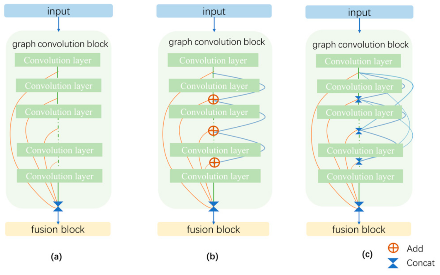
To extract information in different localities and wider ranges, it is often necessary to overlay deeper layers. However, because of the problem of gradient vanishing, excessive numbers of layers will lead to the over-smoothing of node information, eventually leading to degradation in performance. Inspired by the jump connection in CNNs, Xu et al. [23] developed a JK-Nets architecture and applied it to different graph-convolution models. Because the output of the shallow layer was more inclined to represent the local information of different neighborhoods, whereas the deep network was more inclined to represent global information, it was more reasonable to aggregate local and global information together for prediction. JK-Nets aggregate the output of different hidden layers as the input of the final layer (prediction layer). There are three ways to aggregate the output features of hidden layers of a node in JK-Nets architectures, as given below.
- Concat: This method performs a simple merge operation on all output features of hidden layers and obtains input of the prediction layer using a linear transformation. This method is suitable for small graphs or graphs having regular structures and low adaptability.
- Max-pooling: This method selects elements of the layer having the maximum information sequentially. Max-pooling is node-adaptive, and no additional learning parameters are introduced.
- LSTM-Attention: The key to LSTM-attention is the attention coefficient . For the first input to a bidirectional LSTM, each layer generates forward hidden features and backward hidden features . Next, these two features are merged to attain an attention score using linear mapping, which will be input into the SoftMax function and obtain the normalized attention coefficient . is the weighted average of the features of the hidden layers. The formula is as follows.
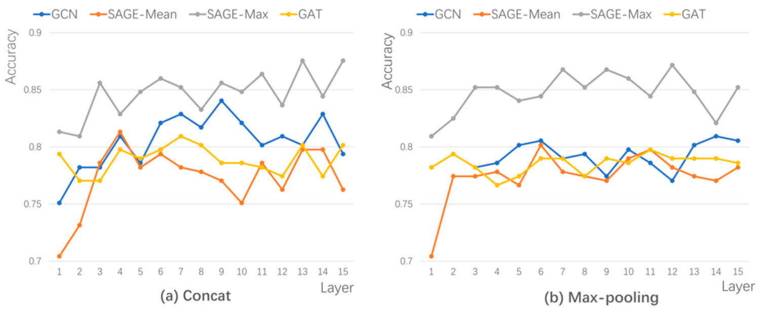
Owing to the high complexity of the LSTM-attention method, the computation process causes the overflow of graphics processing unit (GPU) memory when the model stacks over nine layers; therefore, LSTM-attention was excluded in our study. As shown in Figure 1, the model still maintains a high accuracy rate when the two aggregation methods (Concat and Max-pooling) are superimposed with 15 layers, and the model performance does not degrade significantly. In this study, Concat, with a slightly higher accuracy than Max-pooling, was used to connect the layers.
In addition, Li [25] borrowed some concepts from CNNs—specifically, residual/dense connections and dilated convolutions—and adapted them to the GCN. Extensive experiments were conducted, and the results showed the positive effects of these deep GCN frameworks. Figure 2 compares the three methods of JK-Net, ResNet, and DenseNet. The difference between DenseNet and ResNet is in the methods used for aggregating feature representations. ResNet simply adds all the feature representations, whereas DenseNet conducts a concatenation operation to connect the feature representations, similar to Concat in JK-Nets. In contrast, DenseNet connects and aggregates all hidden layers, but JK-Nets only connects the last layer.
3.2. Dual Graph of Road Network and Its Selection Feature
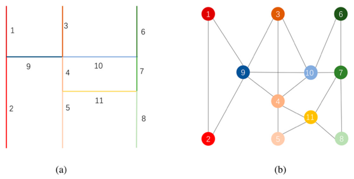
To apply GCNs for road network selection, we abstracted the road network into a graph structure after processing abnormal roads. Currently, two existing methods have been reported in the literature to abstract a road network into a graph.
- Direct representation: Because the road network is naturally a graph structure, it can directly take the road as the edge of the graph and the road intersection as the node.
- Dual representation: The road is abstracted as the node, with the intersection regarded as an edge [46].
In graph theory, nodes are often used to represent target objects, and edges represent the relationships between the objects. The target object of road network selection is a road; therefore, a dual representation that regards roads as nodes may be expected to perform better. In addition, GCNs tend to aggregate the characteristics of nodes rather than edges. In summary, in this study, the road network was abstracted as an undirected unweighted dual graph, as shown in Figure 3, and the problem of road network selection was transformed into a problem of node classification in the GCNs.
The characteristics of roads are the key basis for road network selection, which can quantitatively reflect the significance of roads and guide model training. Yuan et al. [47] evaluated the importance of features through Gini impurity and found that the degree, type, and length parameters of the roads had the greatest influence on the selection results. Notably, Gini impurity refers to the probability of incorrectly classifying a randomly chosen element in the dataset, the smaller the value of which, the better the classification effect becomes. Because the dual graph of a road network can directly express the topological features of a road network, we ignored the degree of roads. Notably, length is an important geometric feature of roads, while the type of road reflects their realistic function, which is regarded as a semantic feature. In summary, we used the road type, length, and coordinates as selection parameters as the node feature representation of the dual graph.
3.3. Design of the Selection Model Structure
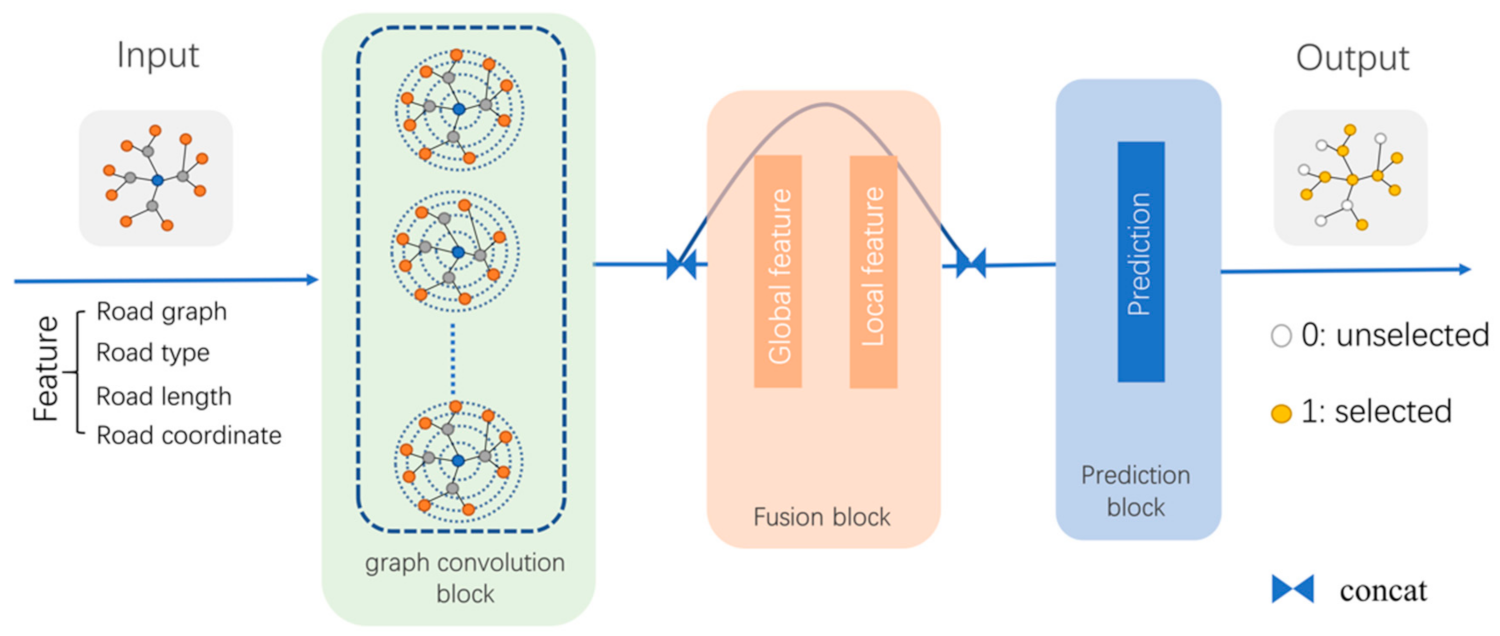
The model was divided into three parts: a graph-convolution block, a fusion block, and a prediction block, as shown in Figure 4. The graph-convolution block was used to extract the local spatial features of the road network, the fusion block was used to fuse global features and different local features, and the prediction block was used to predict the selected results.
Three different deep architectures, JK-Nets, ResNet, and DenseNet, were designed for the graph-convolution block, as shown in Figure 2. These architectures aggregated all the outputs of the graph-convolution layer and served as inputs to the next layer. Notably, the graph-convolution layer extracted the features of the local information, and the deeper the graph-convolution layer, the wider the range that was utilized. Therefore, the outputs of the different graph-convolution layers represented the features of different ranges.
Because the fusion block was connected to the graph-convolution block, the input of the fusion block was the output of the graph-convolution block. The output of the graph-convolution block were the features of different neighborhoods aggregated (by Concat), which were transformed into global features of the graph in the fusion block and then aggregated as the input of the prediction block. Road network selection is a dichotomous problem and, therefore, the output layer of the prediction block has only two neurons, which represent the probability of selection and non-selection.
Because of the complexity of neural networks, implementing neural network models from scratch is time-consuming and laborious. Fortunately, deep learning frameworks carry out the modular encapsulation of various layers or blocks, and these encapsulation blocks can be used to build models quickly and easily. PyTorch Geometric (PyG) is an extended library developed by PyTorch for deep learning on graphs; it supports transferring data into graphs and inputting them to models directly. Therefore, our experiment used PyG to build the GCN models. The blocks mentioned in Figure 4 were programmed successively and contained three types of connections between the layers (JK-Nets, ResNet, and DenseNet) and the four types of neural network architectures (GCN, SAGE-Mean, SAGE-Max, and GAT). The fusion block used a multilayer perceptron (MLP) of a single hidden layer to combine global and local features. The prediction block used the full connection layer and the SoftMax activation function to probabilize the prediction results.
3.4. Accuracy Evaluation Indexes
To evaluate the quality of prediction results, we established two evaluation indices. First, considering the imbalance of positive and negative samples, we adopted the area under the ROC curve (AUC) [48] as the indicator to evaluate the generalization ability of the selection models. Because it is not affected by the distribution of the sample, AUC is a measure commonly used in sample imbalance problems. The value of AUC is the probability that the predicted score of the positive sample is greater than that of the negative sample when selecting a positive sample and a negative sample from the sample pairs. If N samples are sorted from small to large according to the predicted score, the AUC is calculated as follows.
where represents the ordinal number of sample after sorting, with a minimum value of 1 and a maximum value of is the positive example set; and and represent the number of positive and negative samples, respectively.
The second method evaluates the rationality of the selection results. Taking the selection results of experts as the standard, we calculated the selection accuracy, line density, prediction time, and other indicators for comparative analysis. The specific results of the analysis are presented in Section 4.2. Notably, if the positive sample is the selected road and the negative one is the unselected road, the results of model prediction and expert selection can be integrated into four groups: correct selection (true positive, TP), wrong selection (false positive, FP), correct deletion (true negative, TN), and wrong deletion (false negative, FN). A confusion matrix representation is presented in Table 1.
The accuracy of the model refers to the ratio of the number correctly predicted by the selected model to the total number and can be represented as follows.
3.5. Implementation Process
3.5.1. Study Area
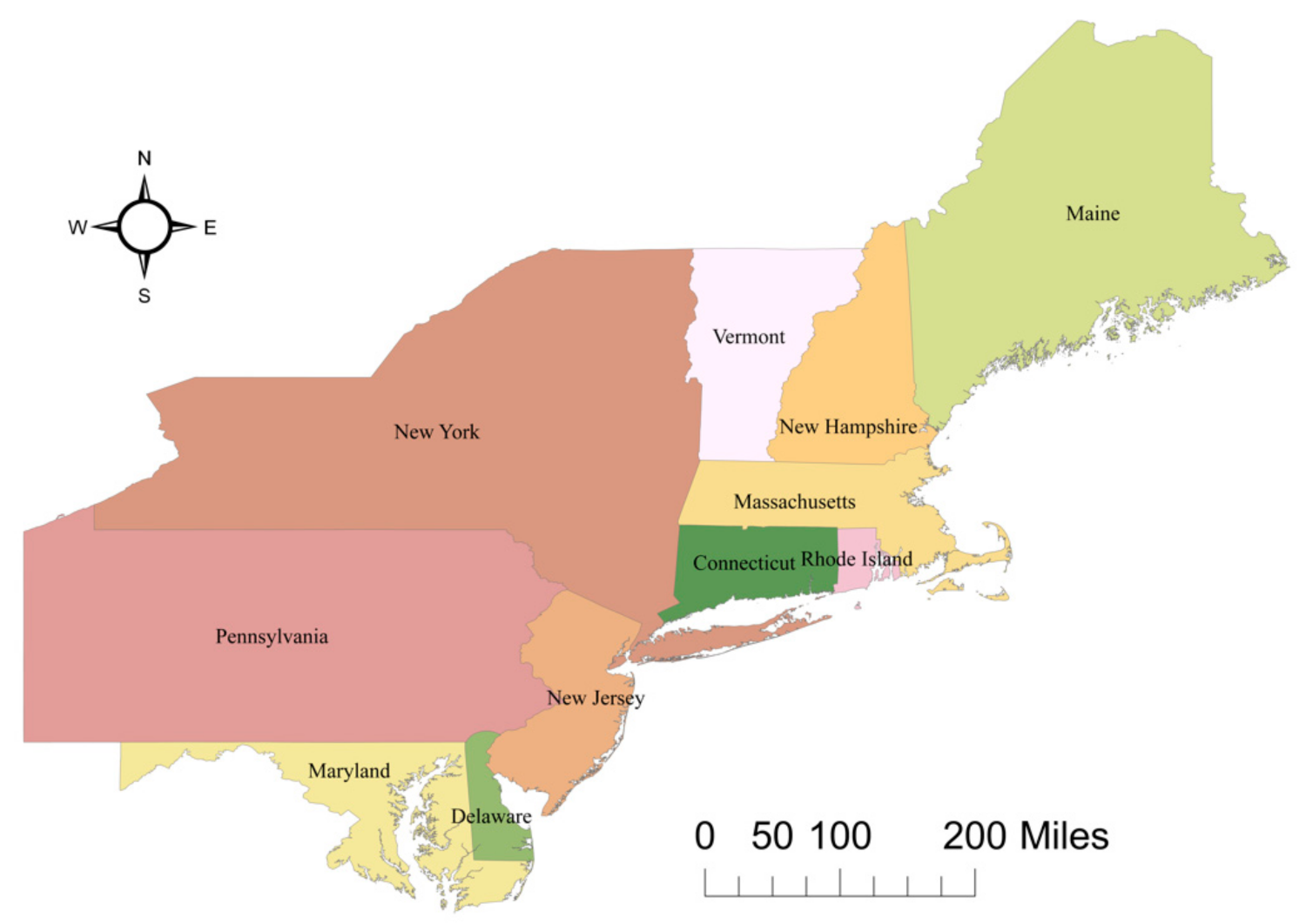
We selected the northeastern region of the United States of America as our study area because the distribution of the road network is comparatively more complex, with different densities and various road structures, while road networks in other regions are too dense and mostly grid structure. Therefore, the road network in the Northeast is more representative, which can show the compatibility of our model. Notably, in this study, we adopted a small-scale road network with less semantic information and more spatial information because our main research purpose was to explore the ability of GCNs to learn the spatial characteristics of road networks. In summary, we downloaded small-scale maps (1:1,000,000 and 1:2,000,000) of a road network in the northeast of the USA, with a total of 5172 roads, including 11 states. The 11 states were (from north to south) Maine, New Hampshire, Vermont, New York, Massachusetts, Rhode Island, Connecticut, Pennsylvania, New Jersey, Delaware, and Maryland (Figure 5).
3.5.2. Data Processing
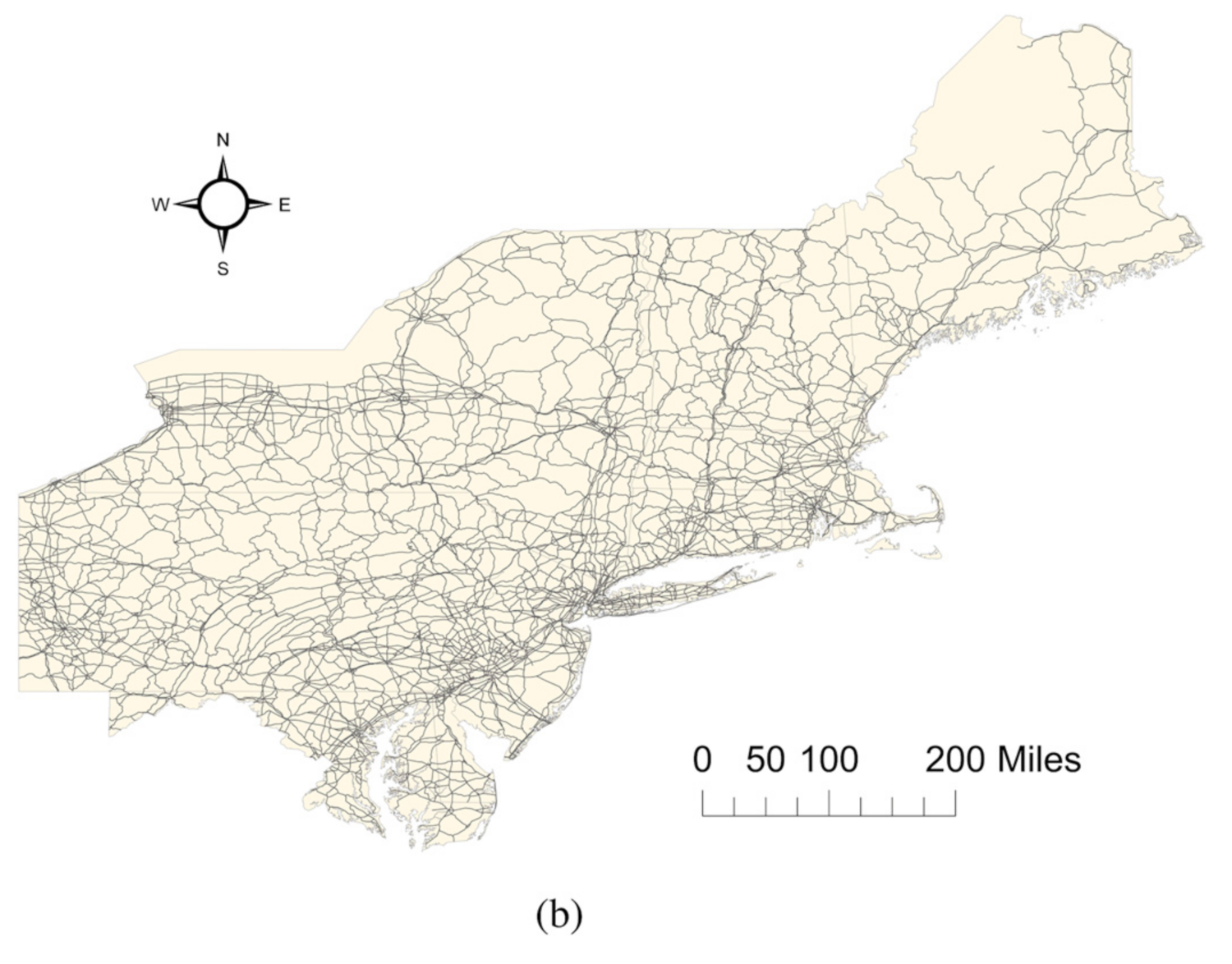
First, we downloaded the small-scale maps at scales of 1:1,000,000 and 1:2,000,000 from the United States Geological Survey (USGS) official website and then used ArcGIS to split the road network in the experimental area, as shown in Figure 6. Figure 6a represents the road network at a scale of 1:1,000,000, and Figure 6b shows a scale of 1:2,000,000.
Notably, the datasets downloaded from the USGS were preprocessed before being input into the model. This procedure mainly included processing abnormal roads, labeling roads, and constructing road features and a dual graph. Specifically, we removed isolated roads by topology inspection and manually labeled all of the roads on the basis of a standard road network. The detailed label work is as follows. A “selection” field of integral type was added to the attribute sheet of 1:100,000 map as the label field, and the value of the “selection” field was assigned as follows. If the path overlapped in the two layers, it was valued as 1; otherwise, it had a value of 0. Finally, a Python program was written to automatically build a bipartite graph. The main tasks of this program were to consider the spatial coordinates, road type, and road length of the road as the selection basis, measure the characteristics of the road, numeralize and normalize the features, generate the edge index by judging the intersection, and generate a bipartite graph based on the node characteristics and edge index.
3.5.3. Model Construction and Training
The graph-convolution blocks were combined into 12 groups on the basis of three deep architectures and four models, and some hyperparameters were used to train these groups for a fair comparison. Hyperparameters refer to the parameters in models that cannot be learned; these parameters can determine the optimal parameters that the model finally learns. They mainly include the activation function, number of hidden layers, number of neurons in hidden layers, and dropout rate. In our study, to reduce the time spent searching, only the hyperparameters of the selection model, other than the activation function, were searched. We adopted the rectified linear unit (ReLU) function in the hidden layer, which is the most commonly used activation function in deep learning models. Using random search for the model parameters, we set 14 layers for the graph-convolution block, a total of 256 neurons in all the hidden layers, and a dropout rate of 0.1. In particular, the number of attention heads was set to four in the GAT architecture.
The purpose of model training is to find the optimal parameters for the selection model, and the backpropagation (BP) algorithm is the main algorithm for training neural network models in deep learning. It quickly calculates the gradient of parameters through the chain rule of derivatives and uses the gradient descent algorithm to update the parameters. Therefore, the BP algorithm was used to train the selection model in this study, and the training process was divided into three steps: forward propagation, back propagation, and parameter update.
4. Results and Discussions
4.1. Predicted Results of Models
Table 2 displays the optimal AUC scores of the 12 models with respect to the validation data. GraphSAGE had the lowest score and the worst performance. The scores of GCN and GAT were as high as 90%, with the GAT model’s scores being slightly higher. Otherwise, the scores of the three deep architectures showed little difference. DenseNet achieved a higher score than the others, among which GAT had the highest score, reaching 91.99%.
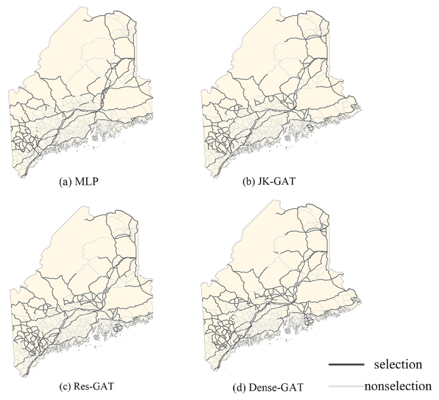
The findings of the above analysis revealed that the GAT model has the best performance; therefore, we used the trained GAT model to predict road network selection in Maine. We also used MLP and compared its selection effects with four other types of GCN models to prove the effectiveness of deepening GCNs; the results are shown in Figure 7.
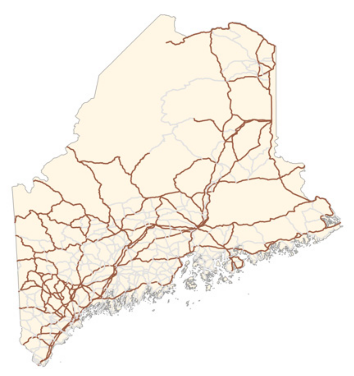
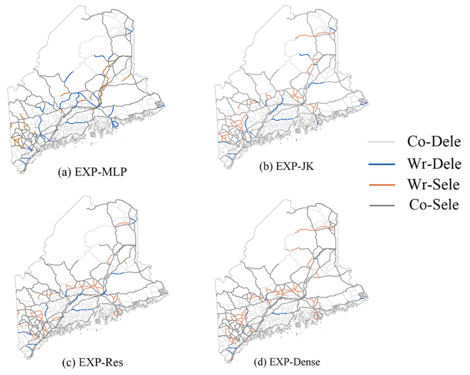
In order to intuitively analyze the selection results, we compared the road network selected by our models with a road network map with a scale of 1:2,000,000 selected by experts (as shown in Figure 8) and thereby obtained Figure 9.
The gray lines in the figure represent the correctly predicted road network; the light gray lines represent the unselected network, and the dark gray lines represent the selected network. The colored lines represent the inaccurately predicted roads; the orange lines represent the inaccurately selected roads, and the blue lines represent the incorrectly deleted roads.
4.2. Analysis and Discussion
To further analyze the quality of the selected results, we used the measures of accuracy rate, line density, and prediction time. Each index was calculated using a Python program (see Table 3).
MLP is a classical neural network model, which includes three parts: an input layer, a hidden layer, and an output layer, like GCNs. The difference between the two models is that MLP cannot directly extract the topological features of road networks, such as degree centrality and closeness centrality. However, end-to-end learning for graph data structure is an advantage of the GCN model, which can directly take the dual graph of the road network as input data and use a graph-convolution operation to extract topological features. As a result, GCNs are less computationally intensive than MLP in the process of data processing.
As for the selection results, the MLP model obtained the lowest accuracy rate (with a rate of 85.83%) and the smallest line density, with incorrect deletion occurring more than incorrect selection. However, in terms of prediction time, MLP was much less time-consuming than GCN. This is because the MLP model structure is relatively simple. The input layer is responsible for processing input data. The hidden layer is usually comprised of multiple layers and is responsible for extracting abstract features from data. The output layer is responsible for calculating the feature representation of the hidden layer and outputting the prediction results. The GCN model is divided into a graph-convolution module, a fusion module, and a prediction module. The graph-convolution module extracts neighbor information and uses different connection strategies to aggregate information in deeper ranger. Therefore, the computational complexity is increased, resulting in a longer prediction time, but the results can also be more accurate.
Among three types of GCN models, it may be observed that the road connectivity of JK-GAT (the combination of JK-Nets and GAT) and Res-GAT (the combination of ResNet and GAT) indicated good results, with relatively balanced rates of selection and deletion. Figure 10 shows a distribution histogram of the predicted results of the GCN models. The predicted results of the first two models were roughly the same, and the distributions of correct selections and wrong selections were relatively uniform, which can maintain the distribution and density of the road network. However, there was a large difference between the numbers of incorrectly selected and deleted roads in Dense-GAT, which may destroy the distribution characteristics of the road network and greatly reduce the selection performance.
Notably, JK-GAT obtained the best performance in terms of accuracy rate (with a rate of 88.12%), whose line density was closest to the results selected by the experts. Moreover, as for the prediction time, Res-GAT obtained the lowest time (2.7 s), while the prediction time of Dense-GAT was as high as 5.84 s because of the complexity of its structure. As mentioned above, every hidden layer is linked to the others in the DenseNet architecture (as shown in Figure 2), while JK-Nets only connects them to the last layer and ResNet simply adds them without Concat, so DenseNet took the longest time.
Through the above analysis, we can draw a conclusion that our models have excellent performance according to the high accuracy rate. Furthermore, the linear density and result figure (Figure 7), which are statistically and visually similar to the results of the experts’ selections, demonstrate that our selection model can extract spatial features. However, more details can still be discussed—for example, whether the selection models we proposed are able to consider geometrical and semantic information.
The Figure 11 below shows the distribution of road types in our experimental area. It may be clearly observed that the more important the road type, the higher the probability of selection. Almost all interstate roads and US Routes were selected, and most of the unselected roads were State Routes.
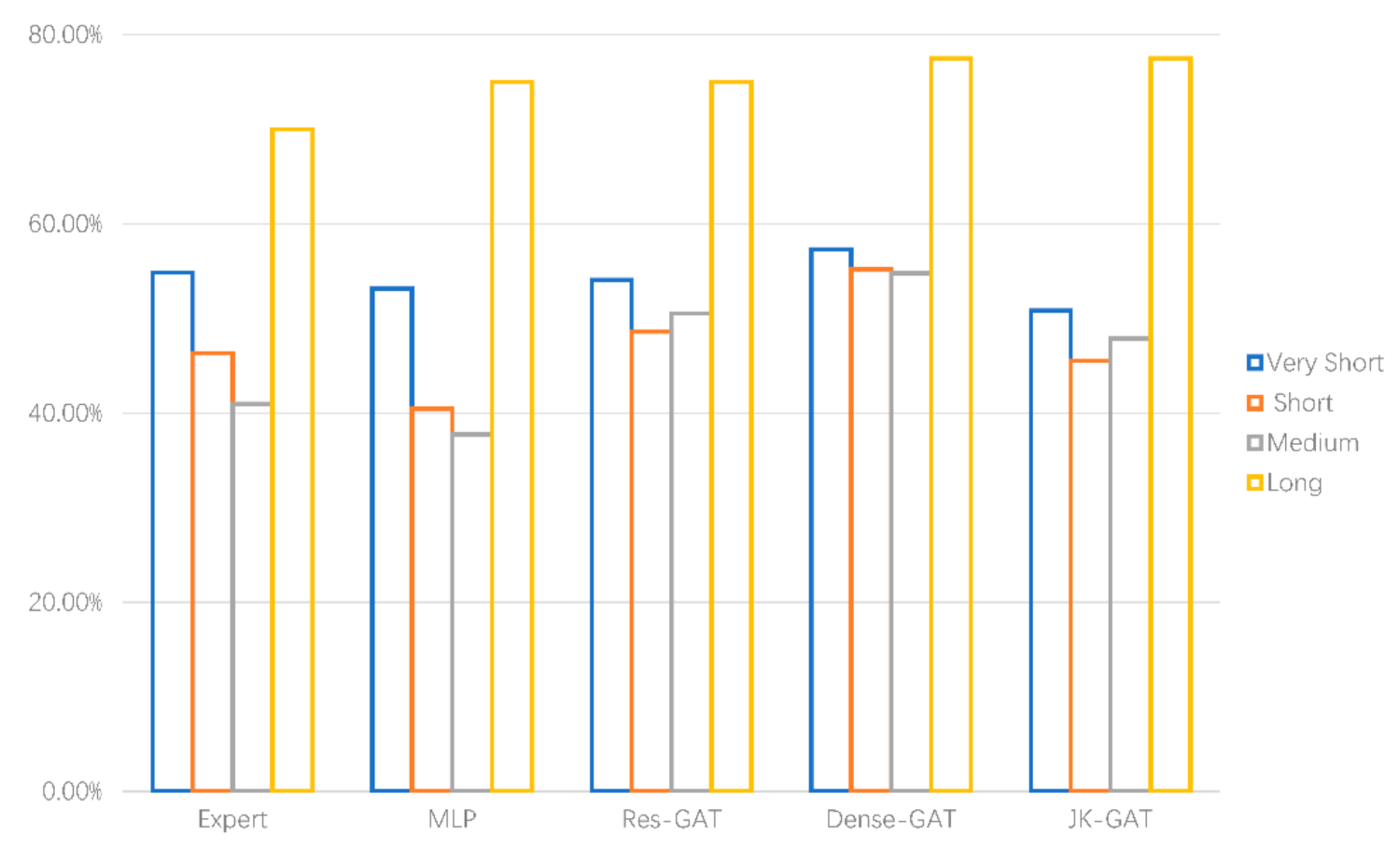
Because the length of road is relatively complex, we divided the entire length into four categories through Natural Breaks, with a distribution diagram shown below (Figure 12). Then, we calculated the rates of selected roads in each group (the selection rate is calculated as Equation (9)). Finally, the selection results of each model are compared with those of the experts. The comparative results are shown below in Table 4 and Figure 13. As may be noted from the figure, the selection results of the four models were very similar to those of experts, without much difference. However, when the road length was considered separately, MLP was closer to expert selection. This also indirectly indicates that topological information had little influence on MLP. In other words, topological information was not a significant feature for deep learning in the MLP model, and our models are more suitable to exploit the topological feature.
SR (Selection Rate) = selected roads/roads in each length group
5. Conclusions and Future Work
This study adopted GCN as a novel deep learning method for automatic road network selection. Road network selection can be regarded as a supervised classification task in intelligent methods, which can be divided into traditional machine learning and deep learning. Traditional machine learning models for classification mainly include SVM, decision tree, and random forest. Deep learning models, mainly including MLP, CNNs, and GCNs, are superior to traditional machine learning models because they reduce the process of manual feature construction (mainly the geometrical and semantic information, except for topological information). Traditional machine learning methods rely heavily on feature engineering. Those features are the basis of model training, and bad feature engineering results in considerable subjectivity of the entire training process. Furthermore, GCNs differ from other deep learning models in that they are able to automatically extract spatial features (especially topological features) through a graph-convolution operation. Other neural network models still have the limitations of traditional machine learning because they transform the graph structure of road networks into a tabular structure by calculating road centrality, density, and other topological indicators and then input them into the model for prediction. We adopted GCNs to select roads because they can directly take the original road data as input and use a graph-convolution operation to construct the spatial features of the road network.
In addition to the theoretical discussion, we have also conducted empirical research. The northeastern region of the United States of America was our experimental area, and 1:100,000- and 1:200,000-scale road networks from the USGS were used as the experimental data to predict and evaluate the proposed deep GCN models. The results showed that the selection accuracy of deep GCN models was as high as 88%, with the connectivity between roads maintained effectively. The density of the road network selected by our models was not much different from that selected by experts, which indicates that our models maintain the distribution characteristics of the road network. In addition, deep architectures such as JK-Nets, ResNet, and DenseNet broke through the three-layer limitation of deep learning models, reaching 14 layers in our experiment. All of the above results indicate that GCNs have the ability to extract the spatial characteristics of road networks, and the deepening methods can effectively solve the problem of gradient vanishing.
However, this study still involves some limitations. First of all, maps with different scales should be explored. We only used a small-scale map, and the selection effect of GCN models in medium and large-scale maps needs to be further explored. Different scales mean different selection and the importance of road features. For example, in small-scale maps, information on shops and traffic flow along the street is not considered. Moreover, the topological characteristics are more complex in large-scale maps. In the future, comparative experiments on different scales should be conducted to explore the applicability of deep GCN models.
Secondly, the use of other deep strategies to connect layers should be investigated. Although the deep strategies discussed in the present work can make GCNs overlay at a deeper level, the improvement of selection accuracy is not obvious. Different methods can be explored in the future, such as a combination with dilated convolutions.
Next, the extensibility of our method has not been discussed. A comparative study on road networks in different regions can be conducted to verify whether GCNs have different performance in different regions or road networks with different characteristics—and, if so, what influences these variances?
Finally, more types of GCN models can be used. In this paper, only four models based on graph convolution were used for comparative experiments. Although GAT achieved the best performance, it requires considerable memory and time, and the selection result is still far from practical application. There are many variations of graph convolution, and further study is required to determine which model is most suitable for road network selection. Indeed, specialized graph-convolution models may be developed for road network selection in future research.
Author Contributions
Conceptualization, Jing Zheng; methodology, Jing Zheng, Ziren Gao, and Jingsong Ma; software, Kang Zhang; validation, Kang Zhang and Jingsong Ma; formal analysis, Jing Zheng; investigation, Kang Zhang; resources, Jie Shen; data curation, Ziren Gao; writing—original draft preparation, Jing Zheng; writing—review and editing, Jing Zheng, Ziren Gao, and Jingsong Ma; supervision, Jingsong Ma; project administration, Jie Shen; funding acquisition, Jie Shen. All authors have read and agreed to the published version of the manuscript.
Funding
This research was funded by the National Natural Science Foundation of China, grant number 41871371.
Institutional Review Board Statement
Not applicable.
Informed Consent Statement
Not applicable.
Data Availability Statement
Not applicable.
Acknowledgments
The authors would like to thank the websites https://gadm.org/ (accessed on 3 May 2020) and https://www.usgs.gov/ (accessed on 3 May 2020) for providing the free maps.
Conflicts of Interest
The authors declare no conflict of interest.
References
- Mackaness, W.A.; Beard, K.M. Use of Graph Theory to Support Map Generalization. Cartogr. Geogr. Inf. Syst. 1993, 20, 210–221. [Google Scholar] [CrossRef]
- Wang, J.Y.; Cui, T.J.; Wang, G.X. Application of Graph Theory in Automatic Selection of Road Network. J. Geomat. Sci. Technol. 1985, 1, 79–86. [Google Scholar]
- Thomson, R.C.; Richardson, D.E. The ‘Good Continuation’Principle of Perceptual Organization Applied to the Generalization of Road Networks. In Proceedings of the ICA 19th International Cartographic Conference, Ottawa, ON, Canada, 14–21 August 1999; pp. 1215–1223. [Google Scholar]
- Thomson, R.; Brooks, R. Generalisation of Geographical Networks. Gen. Geogr. Inf. 2007, 255–267. [Google Scholar] [CrossRef]
- Hu, Y.G.; Chen, J.; Li, Z.L. Selective Omission of Road Features Based on Mesh Density for Digital Map Generalization. Acta Geod. Cartogr. Sin. 2007, 351–357. [Google Scholar] [CrossRef]
- Aurenhammer, F. Voronoi Diagrams—a Survey of a Fundamental Geometric Data Structure. ACM Comput. Surv. 1991, 23, 345–405. [Google Scholar] [CrossRef]
- Yang, M.; Ai, T.H.; Zhou, Q. A Method of Road Network Generalization Considering Stroke Properties of Road Object. Acta Geod. Cartogr. Sin. 2013, 42, 581–587. [Google Scholar]
- Cai, Y.X.; Guo, Q.S. Method For Streets Progressive Selection Based On Neural Network Techniques. J. Geomat. 2008, 05, 24–26. [Google Scholar]
- Liu, K.; Li, J.; Shen, J.; Ma, J.S. Selection of Road Network Using BP Neural Network and Topological Parameters. J. Geomat. Sci. Technol. 2016, 33, 325–330. [Google Scholar]
- Liu, P.; Yuan, L.H.; Zhang, K.; Shen, J.; Ma, J.S. Intelligent Selection of OSM Road Network Based on RBF Neural Network. Geomat. World 2019, 26, 8–13. [Google Scholar]
- Jiang, B.; Harrie, L. Selection of Streets from a Network Using Self-Organizing Maps. Trans. GIS 2004, 8, 335–350. [Google Scholar] [CrossRef]
- Li, M.Z.; Xu, Z.; Li, Z.L.; Zhang, H.; Ti, P. A Hierarchical Random Graph Based Selection Method for Road Network Generalization. J. Geo-Inf. Sci. 2012, 14, 719–727. [Google Scholar] [CrossRef]
- Deng, H.Y.; Wu, F.; Zhai, R.J.; Liu, W.W. A Generalization Model of Road Networks Based on Genetic Algorithm. Geomat. Inf. Sci. Wuhan Univ. 2006, 164–167. [Google Scholar] [CrossRef]
- Wu, Z.H.; Pan, S.R.; Chen, F.W.; Long, G.D.; Zhang, C.Q.; Yu, P.S. A Comprehensive Survey on Graph Neural Networks. IEEE Trans. Neural Netw. Learn. Syst. 2020, 32, 4–24. [Google Scholar] [CrossRef] [Green Version]
- Cho, K.; Merriënboer, B.V.; Gulcehre, C.; Bahdanau, D.; Bougares, F.; Schwenk, H.; Bengio, Y. Learning Phrase Representations Using RNN Encoder-Decoder for Statistical Machine Translation. arXiv 2014, arXiv:1406.1078. [Google Scholar]
- Hochreiter, S.; Schmidhuber, J. Long Short-Term Memory. Neural Comput. 1997, 9, 1735–1780. [Google Scholar] [CrossRef] [PubMed]
- Ai, T.H. Some Thoughts on Deep Learning Enabling Cartography. Acta Geod. Cartogr. Sin. 2021, 50, 1–13. [Google Scholar]
- Kipf, T.N.; Welling, M. Semi-Supervised Classification with Graph Convolutional Networks. arXiv 2016, arXiv:1609.02907. [Google Scholar]
- Wilder, B.; Ewing, E.; Dilkina, B.; Tambe, M. End to End Learning and Optimization on Graphs. Adv. Neural Inf. Process. Syst. 2019, 32, 4672–4683. [Google Scholar]
- Li, Q.M.; Han, Z.C.; Wu, X.M. Deeper Insights into Graph Convolutional Networks for Semi-Supervised Learning. In Proceedings of the Thirty-Second AAAI Conference on Artificial Intelligence, New Orleans, LA, USA, 2–7 February 2018. [Google Scholar]
- Huang, G.; Liu, Z.; Van Der Maaten, L.; Weinberger, K.Q. Densely Connected Convolutional Networks. In Proceedings of the IEEE Conference on Computer Vision and Pattern Recognition, Honolulu, HI, USA, 21–26 July 2017; pp. 4700–4708. [Google Scholar]
- Yu, F.; Koltun, V. Multi-Scale Context Aggregation by Dilated Convolutions. arXiv 2015, arXiv:1511.07122. [Google Scholar]
- Xu, K.; Li, C.T.; Tian, Y.L.; Tomohiro, S.; Kawarabayashi, K.; Jegelka, S. Representation Learning on Graphs with Jumping Knowledge Networks. In Proceedings of the International Conference on Machine Learning, Stockholm, Sweden, 10–15 July 2018; pp. 5453–5462. [Google Scholar]
- He, K.M.; Zhang, X.Y.; Ren, S.Q.; Sun, J. Deep Residual Learning for Image Recognition. In Proceedings of the IEEE Conference on Computer Vision and Pattern Recognition, Las Vegas, NV, USA, 27–30 June 2016; pp. 770–778. [Google Scholar]
- Li, G.H.; Muller, M.; Thabet, A.; Ghanem, B. DeepGCNs: Can GCNs Go As Deep As CNNs? In Proceedings of the IEEE/CVF International Conference on Computer Vision (ICCV), Seoul, Korea, 27 October–3 November 2019. [Google Scholar]
- Hamilton, W.L.; Ying, R.; Leskovec, J. Inductive Representation Learning on Large Graphs. In Proceedings of the 31st International Conference on Neural Information Processing Systems, Long Beach, CA, USA, 4–9 December 2017; pp. 1025–1035. [Google Scholar]
- Veličković, P.; Cucurull, G.; Casanova, A.; Romero, A.; Lio, P.; Bengio, Y. Graph Attention Networks. arXiv 2017, arXiv:1710.10903. [Google Scholar]
- Grover, A.; Leskovec, J. Node2vec: Scalable Feature Learning for Networks. In Proceedings of the 22nd ACM SIGKDD International Conference on Knowledge Discovery and Data Mining, San Francisco, CA, USA, 13–17 August 2016; pp. 855–864. [Google Scholar]
- Guo, M.; Qian, H.Z.; Huang, Z.S.; Liu, H.L.; Ju, J.C. ID3 Decision Tree Oriented Knowledge Reasoning Model and Its Application in Road Network Selection. J. Geomat. Sci. Technol. 2012, 29, 308–312. [Google Scholar]
- Quinlan, J.R. Induction of Decision Trees. Mach. Learn. 1986, 1, 81–106. [Google Scholar] [CrossRef] [Green Version]
- Liu, K.; Ma, J.S. Research on Intelligent Selection of Road Network Automatic Generalization Based on Kernel-Based Machine Learning; Nanjing University: Nanjing, China, 2017. [Google Scholar]
- Gori, M.; Monfardini, G.; Scarselli, F. A New Model for Learning in Graph Domains. In Proceedings of the IEEE International Joint Conference on Neural Networks, Montreal, QC, Canada, 1 July–4 August 2005; Volume 2, pp. 729–734. [Google Scholar]
- Scarselli, F.; Gori, M.; Tsoi, A.C.; Hagenbuchner, M.; Monfardini, G. The Graph Neural Network Model. IEEE Trans. Neural Netw. 2008, 20, 61–80. [Google Scholar] [CrossRef] [PubMed] [Green Version]
- Micheli, A. Neural Network for Graphs: A Contextual Constructive Approach. IEEE Trans. Neural Netw. 2009, 20, 498–511. [Google Scholar] [CrossRef] [PubMed]
- Bruna, J.; Zaremba, W.; Szlam, A.; LeCun, Y. Spectral Networks and Locally Connected Networks on Graphs. arXiv 2013, arXiv:1312.6203. [Google Scholar]
- Belkin, M.; Niyogi, P. Laplacian Eigenmaps and Spectral Techniques for Embedding and Clustering. Proc. Nips 2001, 14, 585–591. [Google Scholar]
- Defferrard, M.; Bresson, X.; Vandergheynst, P. Convolutional Neural Networks on Graphs with Fast Localized Spectral Filtering. Adv. Neural Inf. Process. Syst. 2016, 29, 3844–3852. [Google Scholar]
- Zhang, Z.W.; Cui, P.; Wang, X.; Pei, J.; Yao, X.R.; Zhu, W.W. Arbitrary-Order Proximity Preserved Network Embedding. In Proceedings of the 24th ACM SIGKDD International Conference on Knowledge Discovery & Data Mining, London, UK, 19–23 August 2018; pp. 2778–2786. [Google Scholar]
- Bahdanau, D.; Cho, K.; Bengio, Y. Neural Machine Translation by Jointly Learning to Align and Translate. arXiv 2014, arXiv:1409.0473. [Google Scholar]
- Hamaguchi, T.; Oiwa, H.; Shimbo, M.; Matsumoto, Y. Knowledge Transfer for Out-of-Knowledge-Base Entities: A Graph Neural Network Approach. arXiv 2017, arXiv:1706.05674. [Google Scholar]
- Ying, R.; He, R.; Chen, K.; Eksombatchai, P.; Hamilton, W.L.; Leskovec, J. Graph Convolutional Neural Networks for Web-Scale Recommender Systems. In Proceedings of the 24th ACM SIGKDD International Conference on Knowledge Discovery & Data Mining, London, UK, 19–23 August 2018; pp. 974–983. [Google Scholar]
- Wang, H.W.; Zhang, F.Z.; Wang, J.L.; Zhao, M.; Li, W.J.; Xie, X.; Guo, M.Y. Exploring High-Order User Preference on the Knowledge Graph for Recommender Systems. ACM Trans. Inf. Syst. TOIS 2019, 37, 1–26. [Google Scholar] [CrossRef]
- Wang, M.Q.; Ai, T.H.; Yan, X.F.; Xiao, Y. Grid Pattern Recognition in Road Networks Based on Graph Convolution Network Model. Geomat. Inf. Sci. Wuhan Univ. 2020, 45, 1960–1969. [Google Scholar]
- Jepsen, T.S.; Jensen, C.S.; Nielsen, T.D. Relational Fusion Networks: Graph Convolutional Networks for Road Networks. IEEE Trans. Intell. Transp. Syst. 2020. [Google Scholar] [CrossRef]
- Yu, B.; Yin, H.T.; Zhu, Z.X. Spatio-Temporal Graph Convolutional Networks: A Deep Learning Framework for Traffic Forecasting. arXiv 2017, arXiv:1709.04875. [Google Scholar]
- Xu, Z.B.; Wang, Z.H.; Yan, H.W.; Wu, F.; Duan, X.Q.; Sun, L. A Method for Automatic Road Selection Combined with POI Data. J. Geo-Inf. Sci. 2018, 20, 159–166. [Google Scholar]
- Yuan, L.H.; Ma, J.S. Study on Ensemble Learning and Multi-Parameters System for OSM Road Network Selection; Nanjing University: Nanjing, China, 2018. [Google Scholar]
- Maas, A.L.; Hannun, A.Y.; Ng, A.Y. Rectifier Nonlinearities Improve Neural Network Acoustic Models. In Proceedings of the 30th International Conference on Machine Learning, Atlanta, GA, USA, 17–19 June 2013; Volume 30, pp. 1–6. [Google Scholar]
Figure 1.
Comparison of the JK-Net architecture of (a) Concat and (b) Max-pooling, representing the accuracy of different layers.
Figure 1.
Comparison of the JK-Net architecture of (a) Concat and (b) Max-pooling, representing the accuracy of different layers.

Figure 2.
Different ways to connect deep layers: (a) JK-Net, (b) ResNet, and (c) DenseNet.

Figure 3.
Road network (a) abstracted as an undirected unweighted dual graph (b).

Figure 4.
Components of our selection model.

Figure 5.
Map of the 11 states in the United States of America considered in our study.

Figure 6.
Small-scale map for northeastern United States of America road network: (a) 1:1,000,000 and (b) 1:2,000,000.
Figure 6.
Small-scale map for northeastern United States of America road network: (a) 1:1,000,000 and (b) 1:2,000,000.


Figure 7.
Maps with road network obtained using different models: (a) multilayer perceptron MLP; (b) JK-GAT; (c) Res-GAT; and (d) Dense-GAT.
Figure 7.
Maps with road network obtained using different models: (a) multilayer perceptron MLP; (b) JK-GAT; (c) Res-GAT; and (d) Dense-GAT.

Figure 8.
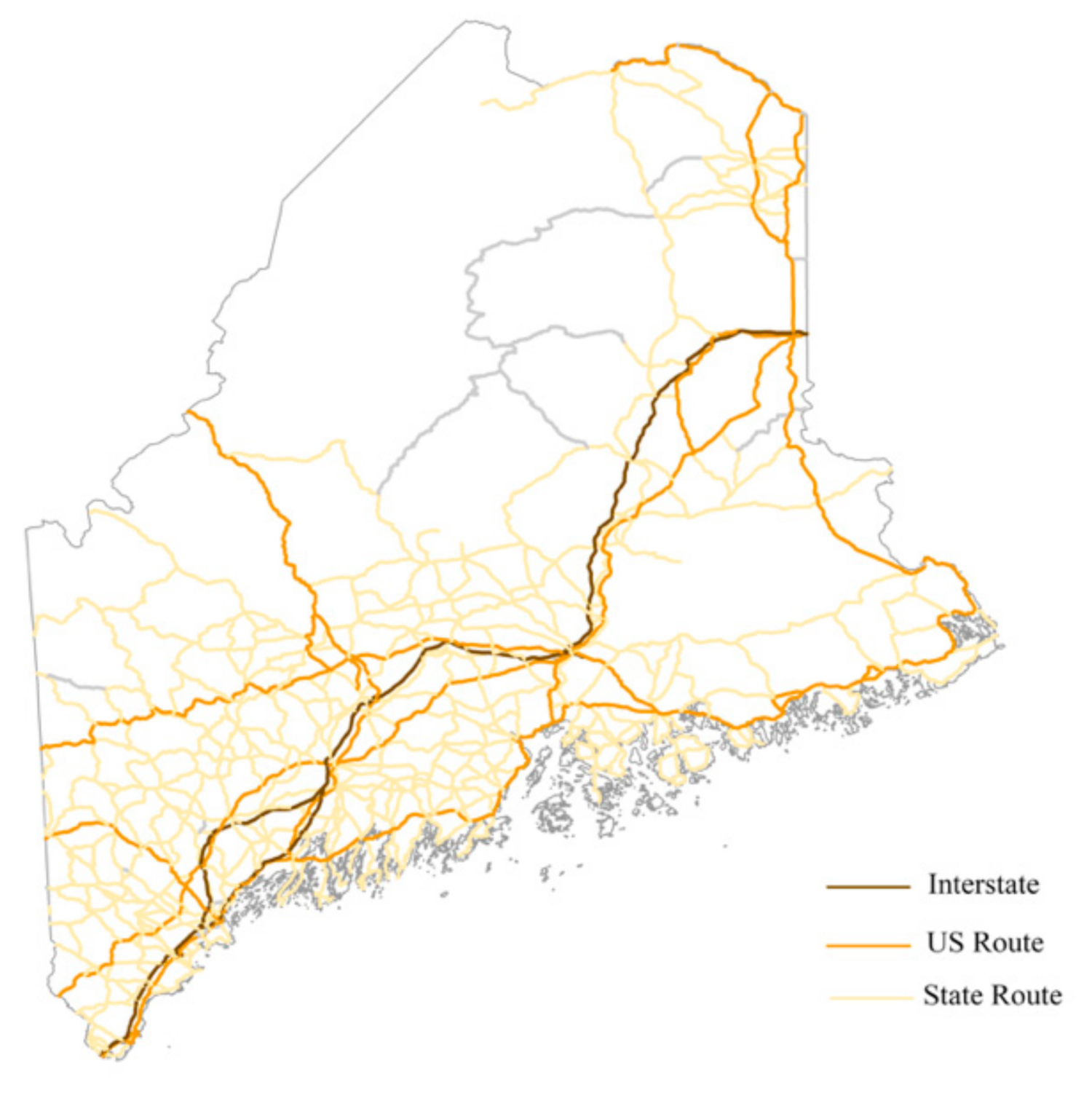
Standard road network map at 1:2,000,000 scale in the Maine area.

Figure 9.
Combinations of the road network obtained using different models and the road network selected by experts: (a) expert and multilayer perceptron (EXP-MLP); (b) expert and JK-GAT (EXP-JK); (c) expert and Res-GAT (EXP-Res); and (d) expert and Dense-GAT (EXP-Dense). Co-Dele represents correctly deleted roads, Wr-Dele represents incorrectly deleted roads, Wr-Sele represents incorrectly selected roads, and Co-Sele represents correctly selected roads.

Figure 10.
Distribution histogram of the predicted results of the GCN models.

Figure 11.
Distribution of road types in Maine.

Figure 12.
Distribution of road length in Maine.

Figure 13.
Histogram of selection rate of each length group for different models.


Table 1.
Confusion matrix representation of the classification model.
| Model | Unselect (0) | Select (1) | |
|---|---|---|---|
| Expert | |||
| Unselect (0) | Correct deletion (TN) | Wrong selection (FP) | |
| Select (1) | Wrong deletion (FN) | Correct selection (TP) | |
Table 2.
Optimal area under the ROC curve (AUC) scores of the 12 models.
| Convolution | GCN | SAGE-Mean | SAGE-Max | GAT | |
|---|---|---|---|---|---|
| Connection | |||||
| JK | 88.38 | 87.76 | 87.04 | 91.68 | |
| Res | 89.41 | 88.89 | 86.67 | 91.25 | |
| Dense | 89.70 | 89.49 | 84.92 | 91.99 | |
Table 3.
Accuracy rate, line density, and prediction time of different models calculated using the Python programming language.
Table 3.
Accuracy rate, line density, and prediction time of different models calculated using the Python programming language.
| Incorrect Deletion | Incorrect Selection | Accuracy Rate (%) | Density (km/km2) | Prediction Time (s) | |
|---|---|---|---|---|---|
| Expert | - | - | - | 0.0431 | - |
| MLP | 109 | 71 | 85.83 | 0.0405 | 0.125 |
| JK-GAT | 82 | 69 | 88.12 | 0.0453 | 3.59 |
| Res-GAT | 65 | 89 | 87.88 | 0.0471 | 2.57 |
| Dense-GAT | 40 | 120 | 87.41 | 0.0509 | 5.84 |
Table 4.
Selection rate of each length group for different models.
| SR | Very Short | Short | Medium | Long |
|---|---|---|---|---|
| Expert | 54.85% | 46.31% | 40.96% | 70% |
| MLP | 53.16% | 40.46% | 37.77% | 75% |
| JK-GAT | 50.85% | 45.55% | 47.87% | 77.5% |
| Res-GAT | 54.08% | 48.6% | 54.79% | 75% |
| Dense-GAT | 57.32% | 55.22% | 54.79% | 77.45% |
Publisher’s Note: MDPI stays neutral with regard to jurisdictional claims in published maps and institutional affiliations. |
© 2021 by the authors. Licensee MDPI, Basel, Switzerland. This article is an open access article distributed under the terms and conditions of the Creative Commons Attribution (CC BY) license (https://creativecommons.org/licenses/by/4.0/).
Share and Cite
MDPI and ACS Style
Zheng, J.; Gao, Z.; Ma, J.; Shen, J.; Zhang, K. Deep Graph Convolutional Networks for Accurate Automatic Road Network Selection. ISPRS Int. J. Geo-Inf. 2021, 10, 768. https://0-doi-org.brum.beds.ac.uk/10.3390/ijgi10110768
AMA Style
Zheng J, Gao Z, Ma J, Shen J, Zhang K. Deep Graph Convolutional Networks for Accurate Automatic Road Network Selection. ISPRS International Journal of Geo-Information. 2021; 10(11):768. https://0-doi-org.brum.beds.ac.uk/10.3390/ijgi10110768
Chicago/Turabian StyleZheng, Jing, Ziren Gao, Jingsong Ma, Jie Shen, and Kang Zhang. 2021. "Deep Graph Convolutional Networks for Accurate Automatic Road Network Selection" ISPRS International Journal of Geo-Information 10, no. 11: 768. https://0-doi-org.brum.beds.ac.uk/10.3390/ijgi10110768
Note that from the first issue of 2016, this journal uses article numbers instead of page numbers. See further details here.