Watershed Drought and Ecosystem Services: Spatiotemporal Characteristics and Gray Relational Analysis

Abstract

This study explored the spatiotemporal characteristics of drought and ecosystem services (using soil conservation services as an example) in the YanHe Watershed, which is a typical water basin in the Loess Plateau of China, experiencing soil erosion. Herein, soil conservation was simulated using the Soil and Water Assessment Tool (SWAT), and the relationship between drought, soil conservation services, and meteorological, vegetation, and other factors since the implementation of the ‘Grain for Green’ Project (GFGP) in 1999, were analyzed using the gray relational analysis (GRA) method. The results showed that: (1) The vegetation cover of the Watershed has increased significantly, and evapotranspiration (ET) increased by 14.35 mm·a⁻¹, thereby increasing water consumption by 8.997 × 10⁸ m³·a⁻¹ (compared to 2000). (2) Drought affected 63.86% of the watershed area, gradually worsening from south to north; it decreased in certain middle areas but increased in the humid areas on the southern edge. (3) The watershed soil conservation services, measured by the soil conservation modulus (SCM), increased steadily from 116.87 t·ha⁻¹·a⁻¹ in 2000 to 412.58 t·ha⁻¹·a⁻¹ in 2015, at a multi-year average of 235.69 t·ha⁻¹·a⁻¹, and indicated great spatial variations, with a large variation in the downstream and small variations in the upstream and midstream areas. (4) Integrating normalized difference vegetation index (NDVI) data into SWAT model improved the model simulation accuracy; during the calibration period, the coefficient of determination (R²) increased from 0.63 to 0.76 and Nash–Sutcliffe efficiency (NSE) from 0.46 to 0.51; and during the validation period, the R² increased from 0.82 to 0.93 and the NSE from 0.57 to 0.61. (5) The GRA can be applied to gray control systems, such as the ecosystem; herein, vegetation cover and drought primarily affected ET and soil conservation services. The analysis results showed that vegetation restoration enhanced the soil conservation services, but increased ET and aggravated drought to a certain extent. This study analyzed the spatiotemporal variations in vegetation coverage and the response of ET to vegetation restoration in the YanHe Watershed, to verify the significant role of vegetation restoration in restraining soil erosion and evaluate the extent of water resource consumption due to ET in the semi-arid and semi-humid Loess-area basin during the GFGP period. Thus, this approach may effectively provide a scientific basis for evaluating the ecological effects of the GFGP and formulating policies to identify the impact of human ecological restoration on ecosystem services.

1. Introduction

Ecosystem services (ESs) are defined as “the natural environmental conditions and effects that are formed and maintained by ecosystems and ecological processes and upon which people rely for existence”; they are the benefits that humans gain directly or indirectly from the ecosystem [1]. Based on their contribution to human beings, ESs can be divided into four categories: Supply, regulation, support, and cultural services. Soil conservation services refer to the ability of the ecosystem to control and prevent soil erosion, and store and maintain sediments. As an important regulating service, it helps prevent regional land degradation and reduce the risk of flooding [2]. With the launch of the Millennium Ecosystem Assessment (MEA), particularly the 2003 report, the study of ESs has become a research hotspot in the field of global change. The Loess Plateau in China is located in an ecologically sensitive area, with the coexistence of drought and soil erosion [3,4]. Drought can lead to vegetation degradation [5], reduction of net primary productivity of vegetation [6], land desertification [7], and soil erosion [8] in the natural ecosystem, and affect the supply of water resources [9], agricultural production [10], and energy and power supply [11] in the socioeconomic system. Soil erosion not only causes land degradation [12] and soil fertility decline [13] and affects agricultural production and food security [14], but also causes eutrophication of water bodies [15], siltation of reservoir channels [16], aggravation of flood disasters [17], and other problems in downstream areas. Because of these ecological problems, research on ESs in ecologically fragile areas has become a focus in academic research.

Since the 1970s, the Chinese government has adopted several soil and water conservation measures, including the construction of terraces and silt dams, to mitigate severe soil erosion [18]. In 1999, the government proposed and implemented a series of large-scale ecological modification projects, such as the ‘Grain for Green’ Project (GFGP) [19]. Relevant studies [20,21,22] have shown that the GFGP has significantly increased vegetation coverage, alleviated soil erosion, improved the ecological environment, and enhanced functioning of ecological services in the Loess Plateau. In the global terrestrial ecosystem, vegetation restoration is a primary method to prevent soil erosion, and the study of its impact on ESs has received increasing focus. Fu et al. [23] reported that vegetation has significantly improved in typical regions of the GFGP on the Loess Plateau, and soil conservation, hydrologic regulation, and carbon sequestration services have increased by varying degrees. Wang et al. [24] studied Yulin City in particular and found that soil erosion followed a downward trend with increasing normalized difference vegetation index (NDVI) values, and its temporal and spatial variations were primarily related to rainfall, slope, and land use. Kervroëdan et al. [25] revealed that vegetation-controlled runoff and erosion in the Loess Belt in Europe, by increasing hydraulic roughness and sediment retention; the ability of vegetation to control soil erosion increased with an increase in stem density, diameter, and leaf area. Gashaw et al. [26] reported that the reclamation of cultivated land and degradation of vegetation in the Andassa Watershed in Ethiopia increased food production and pollination, but degraded several other ESs to varying levels, indicating that vegetation has an irreplaceable role in regional ecosystems. Most studies on soil erosion control have analyzed the effect of vegetation macroscopically, with few studies examining the spatial and temporal distribution characteristics and influencing factors of vegetation restoration on soil conservation services.

Tobler’s First Law of Geography [27] states that “everything is related to everything else”. Vegetation restoration enhances soil conservation and reduces sediment load. However, vegetation growth increases regional evapotranspiration (ET) by changing surface roughness, surface reflectivity, interception of precipitation, and transpiration [28], which further aggravates regional water shortages [29] and the degree of drought [30]. Similar results have been reported by other researchers [31,32]. Drought is a major meteorological disaster affecting socioeconomic and natural ecosystems. Drought indices are the primary tools to identify and monitor drought and investigate drought characteristics [33]. Commonly used drought indices include the standardized precipitation index (SPI), standardized precipitation evaporation index (SPEI), evaporative stress index (ESI), and Palmer drought severity index (PDSI). Although the SPI index is widely accepted by climatologists and hydrologists, it is based only on accumulated precipitation and does not consider the impact of water demand on drought. To overcome this, the SPEI was developed by Vicente-Serrano et al. [34] to incorporate potential evapotranspiration (PET). Potop et al. [35] showed that the SPEI might better characterize drought in areas with significantly warm climates; however, it requires long time-series data. Most studies calculate the SPI and SPEI using data obtained from meteorological stations. Moreover, due to the inconsistent research scales, the drought rules observed at the point scale are not scientifically reliable for evaluating vegetation restoration and policymaking at the regional scale [36]. Remote sensing data provide multi-resolution (spectral and spatial) and abundant information [37]; hence, the construction of drought indices based on remote sensing data has gradually become the primary method for evaluating drought. The ESI is the ratio of actual to PET and can monitor drought caused by multiple factors, such as decreased precipitation and increased radiation [38]. The ESI has been widely used in several drought monitoring studies [39,40]. Yoon et al. [40] identified the advantages of ESI over other satellite-based drought assessment indices and explored its applicability as a new indicator of agricultural drought monitoring. Liu et al. [41] showed that the ESI indicated drought in arid river basins of Northwest China better than RDI. Therefore, in this study, the ESI was constructed to monitor drought in the YanHe Watershed.

The impact of vegetation restoration on spatiotemporal pattern changes of drought and soil conservation requires urgent investigation because of the adverse effects of drought on ecology and socio-economy, and the significant impact of vegetation restoration in enhancing soil conservation services [42]. However, the ecosystem is a gray system with complex response mechanisms between drought, soil conservation, and their respective influencing factors. Herein, we introduced the GRA method to evaluate the effect of vegetation restoration on drought and supply of ecosystem services. The ecosystem service cascade [43] indicates that the process by which humans obtain ESs from natural ecosystems [44] and is a gradual transformation of ecosystem structure and processes. Therefore, this study analyzed the process of increasing water consumption through vegetation restoration using remote sensing data, and quantified soil conservation services using the Soil and Water Assessment Tool (SWAT) model. The cascade model of process–effect–service was adopted to analyze drought and soil conservation services in the YanHe Watershed.

This study aimed to: (1) Understand the spatiotemporal variations of vegetation coverage and the response of ET to vegetation restoration in the YanHe Watershed since 2000; (2) explore the spatiotemporal characteristics and evolutionary trends of drought in the basin; and (3) evaluate spatiotemporal variations and the influencing factors of soil conservation services. The results of this study were used to analyze the excessive consumption of water resources caused by vegetation restoration in the YanHe Watershed during 2000–2015, and the significant role of vegetation restoration in restraining soil erosion. The research results are conducive to comprehensively evaluate the ecological effects of the GFGP, thereby provide a reference for ecological control on the Loess Plateau and guide the construction of ecological civilization.

2. Materials and Methods

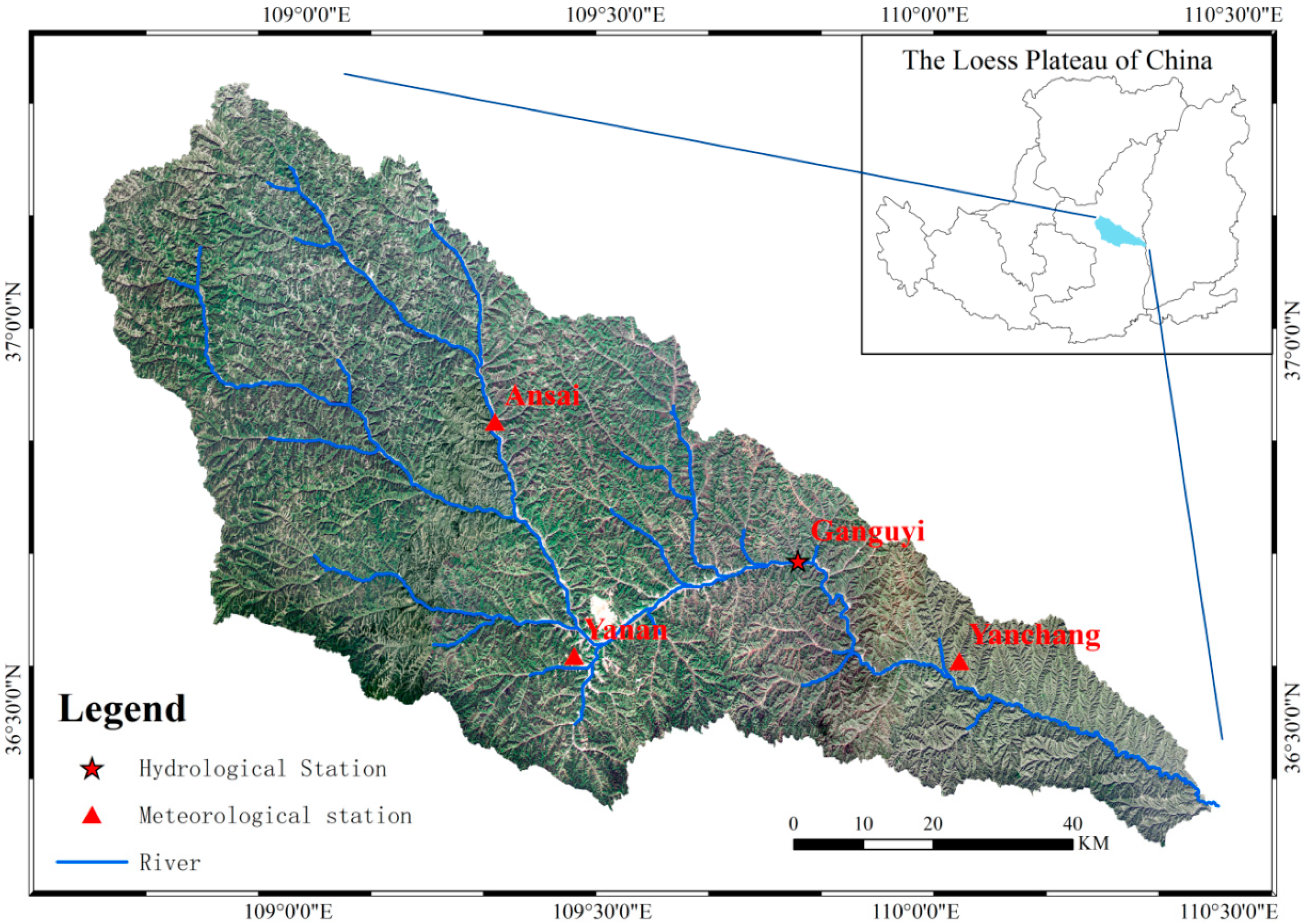
2.1. Overview of the Study Area

The YanHe River is a primary tributary in the middle reaches of the Yellow River; it originates from the Baiyu Mountains in Jingbian County, Shaanxi Province, and flows through the Zhidan, Ansai, and Baota counties [45]. After 286.9 km, it flows into the Yellow River in Yanchang County. The YanHe Watershed (36°27′–37°58′ N, 108°41′–110°29′ E) covers 7725 km² and has an altitude of 461–1787 m (average elevation 1212 m) (Figure 1), with an average slope of 4.3% and gully density of 4.7 km/km². The regional terrain is high in the northwest and low in the southeast, with forms including the hilly and gully regions (lower reaches), valley and plain regions (upper reaches), and residual loess platform regions (middle reaches). The study area lies in a warm temperate zone that has a continental semi-arid monsoon climate, with an average annual precipitation of 509 mm, approximately 78% of which occurs between June and October as rainstorms. The average annual temperature is 8.8–10.2 °C, average annual evaporation 1000 mm, and annual total radiation 125–134 kcal/cm² [46]. The main soil type is loose and soft loessial soil with poor erosion resistance. The YanHe Watershed is a part of the Loess Hilly-Gully Region, with fragmented landforms and crisscross gullies. Soil erosion is most severe in the YanHe Watershed area of the Loess Plateau, occurring in approximately 80% of the total area [47]. The GFGP, by implementing the largest set of revegetation measures in the YanHe Watershed, has changed the vegetation cover since 1999. Vegetation types vary with environmental gradients; steppes and desert steppes occur in the northwest, temperate forest-steppes in the middle, and warm temperate-deciduous broadleaf and mixed coniferous-deciduous broadleaf forests in the southeast of the watershed.

2.2. Data Sources and Preprocessing

This study utilized multiple datasets, including the digital elevation model (DEM), meteorological, hydrological, soil, land use, vegetation, and ET data. (1) DEM data, with a resolution of 30 m, were downloaded from the Geospatial Data Cloud (http://www.gscloud.cn/). (2) Soil data were derived from the China Soil Dataset based on the World Soil Database (HWSD) of the National Tibetan Plateau Data Center (http://westdc.westgis.ac.cn/). (3) Land use data, with a resolution of 30 m, were downloaded from the Resource and Environmental Science Data Center of the Chinese Academy of Sciences (http://www.resdc.cn/) and reclassified into six land use types. (4) Meteorological data from 1999 to 2015, including daily precipitation, relative humidity, wind speed, maximum and minimum temperature (solar radiation data simulated by SWAT weather generator), were downloaded from the China Meteorological Data Sharing Network (https://data.cma.cn/). (5) Hydrological data for 2000–2015, including daily runoff and sediment transport, of the Ganguyi Hydrological Station were sourced from the ‘Statistical Yearbook of Hydrology of the People’s Republic of China; (6) Vegetation and ET data for 2000–2015 were obtained from MOD13 (16 days/250 m) and MOD16 (8 days/500 m, yearly/500 m), released by the National Aeronautics and Space Administration (NASA) (https://search.earthdata.nasa.gov/search). The MODIS Re-projection Tools provided by NASA were used to convert the original sinusoidal projection of the MOD13/16 datasets to Universal Transverse Mercator projection (WGS_84_UTM_Zone_49N). The corresponding MODIS products were combined to obtain the monthly NDVI and ET levels of the watershed, based on the Maximum Value Composites and Extract Multi Values to Points tools, respectively, through masking.

2.3. Research Methods

2.3.1. Gray Relational Analysis

Gray relational analysis (GRA) is a multivariate statistical analysis method that assesses the degree of correlation among factors according to their similarity or difference in development trends [48]. As the similarity among the geometric shape of the time series increases, the correlation among these factors becomes more significant. Based on this principle, the major and minor factors that affect the system’s development can be determined. According to Gray System Theory, ecosystems with complicated factor relationships and unclear internal principles are gray control systems. Accounting for the interference of unknown and undetermined factors has increased our understanding of ESs [49]. Gray relational analysis is also suitable for small data samples that do not meet standard distribution laws. While the number of GRA calculations is relatively small, the results are consistent with the qualitative analysis results. Therefore, GRA can be used to analyze the impact of vegetation restoration on drought and supply of ESs. Evaluations using this method are usually based on the gray relational coefficient, degree, and sequence. The specific steps are as follows:

• The evaluation criterion (reference sequence) and evaluation object (comparison sequence) were determined.
• The difference in absolute values was reduced by unifying the data into an approximate range, focusing on data changes and trends.
• The gray relational coefficient, ξ_i(k), was calculated as

  $${\xi }_i\left(k\right)=\frac{{\min }_i{\min }_k\left|y\left(k\right)-x_i\left(k\right)\right|+\rho {\max }_{i}ma{k}_k\left|y\left(\mathrm{k}\right)-x_i\left(k\right)\right|}{\left|y\left(k\right)-x_i\left(k\right)\right|+\rho {\max }_{i}ma{k}_k\left|y\left(\mathrm{k}\right)-x_i\left(k\right)\right|}$$

  (1)

  where ξ_i(k) is the correlation coefficient between reference sequence y(k) and several comparison sequences x₁, x₂, K, and x_n at each moment; ρ is the distinguishing coefficient; usually ρ = 0.5.
• The gray relational degree, r_i, was obtained as a quantitative expression of the degree of association between the reference and comparison sequences as

  $${\mathrm{r}}_i=\frac{1}{n}{\displaystyle {\sum }_{k=1}^n{\xi }_i\left(k\right)}$$

  (2)

  where r_i is the gray correlation degree.
• A correlation sequence of the evaluation subject was established according to the calculated value of the gray relational degree.

2.3.2. Drought Index Based on Remotely Sensed Data

The evaporative stress index (ESI) was used to assess the degree of drought, and the data source was the MOD16 product, which has a good simulation effect on land ET. The ESI considers the role of ET in reflecting the response of vegetation and soil moisture to drought, as the ratio of ET to PET reflects water supply and demand and responds rapidly to water consumption by plants. Anderson et al. [50] standardized the ratio of actual ET to PET (f_PET), which was termed the evaporative stress index (ESI), calculated as follows:

$${\mathrm{ESI}}^{\left(i\right)}=\frac{f_{PET}^{\left(i\right)}-\overline{f_{PET}}}{{\alpha }_{f_{PET}}},i=1,2,\dots ,N$$

(3)

where N is the length of the data sequence, $\overline{f_{PET}}$ the mean $f_{PET}^{\left(i\right)}$, and α_fPET the standard deviation $f_{PET}^{\left(i\right)}$. A positive ESI indicates that the area is wet, while a negative ESI indicates that the area is dry; the specific correspondence is shown in

Table 1. Drought category according to evaporative stress index (ESI).

ESI	Drought Category
ESI ≥ 0	–
−1.0 < ESI < 0	Mild drought
−1.5 < ESI ≤ −1.0	Moderate drought
−2.0 < ESI ≤ −1.5	Severe drought
ESI ≤ −2.0	Extreme drought

.

2.3.3. Soil Conservation Services Assessment

The SWAT model was used to simulate soil conservation services in the YanHe Watershed. The SWAT model, with a strong physical mechanism [51], is a long time-series watershed-scale distributed hydrological model developed by the United States Department of Agriculture-Agricultural Research Center (USDA-ARC) based on the Simulator Water Resources in Rural Basins (SWRRB) model [52]. It has been widely used in the simulation and prediction of hydrological processes [53] and is highly applicable to the Loess Plateau [54,55]. Equation (4) calculates the actual soil erosion using the Modified Universal Soil Loss Equation (MUSLE). This study assumed the absence of vegetation cover when calculating the potential soil erosion. Equation (5) presents the calculation of the amount of soil conservation.

$$\mathrm{sed}=11.8·{\left(Q_{surf}·q_{peak}·are{a}_{hru}\right)}^{0.56}·K_{USLE}·{\mathrm{C}}_{USLE}·P_{USLE}·L{S}_{USLE}·CFRG$$

(4)

$${\mathrm{sed}}_c=11.8·{\left(Q_{surf}·q_{peak}·are{a}_{hru}\right)}^{0.56}·K_{USLE}·\left(1-{\mathrm{C}}_{USLE}\right)·P_{USLE}·L{S}_{USLE}·CFRG$$

(5)

where sed is the actual amount of soil erosion (metric tons), sed_c the amount of soil conservation, Q_surf the surface runoff volume (mm·ha⁻¹), p_each the peak runoff rate (m³·s⁻¹), area_hru the area of the hydrological response unit (HRU) (ha), K_USLE the USLE (universal soil loss equation) soil erodibility factor, C_USLE the USLE cover and management factor, P_USLE the USLE support practice factor, LS_USLE the USLE topographic factor, and CFRG the coarse fragment factor.

The calibration and validation procedures were based on the SUFI-2 algorithm of the SWAT-CUP [56]. The Nash–Sutcliffe efficiency (NSE) and the coefficient of determination (R²) were used to evaluate the simulation accuracy of the SWAT model.

$$\mathrm{NSE}=1-\frac{{\displaystyle {\sum }_{i=1}^n}{\left(Q_{mi}-Q_{oi}\right)}^2}{{\displaystyle {\sum }_{i=1}^n}{\left(Q_{oi}-Q_o\right)}^2}$$

(6)

$${\mathrm{R}}^2=\frac{{\left[{\displaystyle {\sum }_{i=1}^n}\left(Q_{oi}-Q_o\right)\left(Q_{mi}-Q_m\right)\right]}^2}{{\displaystyle {\sum }_{i=1}^n}{\left(Q_{oi}-Q_o\right)}^2{\displaystyle {\sum }_{i=1}^n}{\left(Q_{mi}-Q_m\right)}^2}$$

(7)

where n is the number of observations; Q_oi and Q_mi are observed and predicted values at time i, respectively; Q_o and Q_m are the means of the observed and predicted values, respectively; NSE is the performance of the model output relative to the mean of the observed data; and R² is the consistency of the trend between the observed and predicted values. Generally, the model performance was considered ‘satisfactory’, if R² and NSE values were >0.5 for a monthly time-step [57].

The ArcSWAT2012 software was used to construct the SWAT model of the YanHe Watershed. Flow direction and accumulation were calculated based on DEM and the river network of the basin was extracted with 10,000 ha as the minimum catchment area threshold. The whole basin was divided into 47 sub-basins [58]; by superimposing land use, soil, and slope data, the 47 sub-basins were further divided into 1511 HRUs [59]. Finally, attribute data, such as soil and weather databases, and weather generators, were imported into the SWAT model. The first year (2000) was used as a warm-up period to mitigate the initial conditions. The SWAT parameters were calibrated using monthly sediment data from the Ganguyi station for a period of eight years (2001–2008) and then validated using monthly sediment data for seven years (2009–2015). The model output included monthly runoff, sediment, and other data for each HRU during the simulation period. Based on previous studies [60], the soil conservation modulus (SCM) was divided into five gradients: Lower SCM (0–250 t·ha⁻¹), low SCM (250–500 t·ha⁻¹), medium SCM (500–750 t·ha⁻¹), high SCM (750–1000 t·ha⁻¹), and higher SCM (1000–1500 t·ha⁻¹).

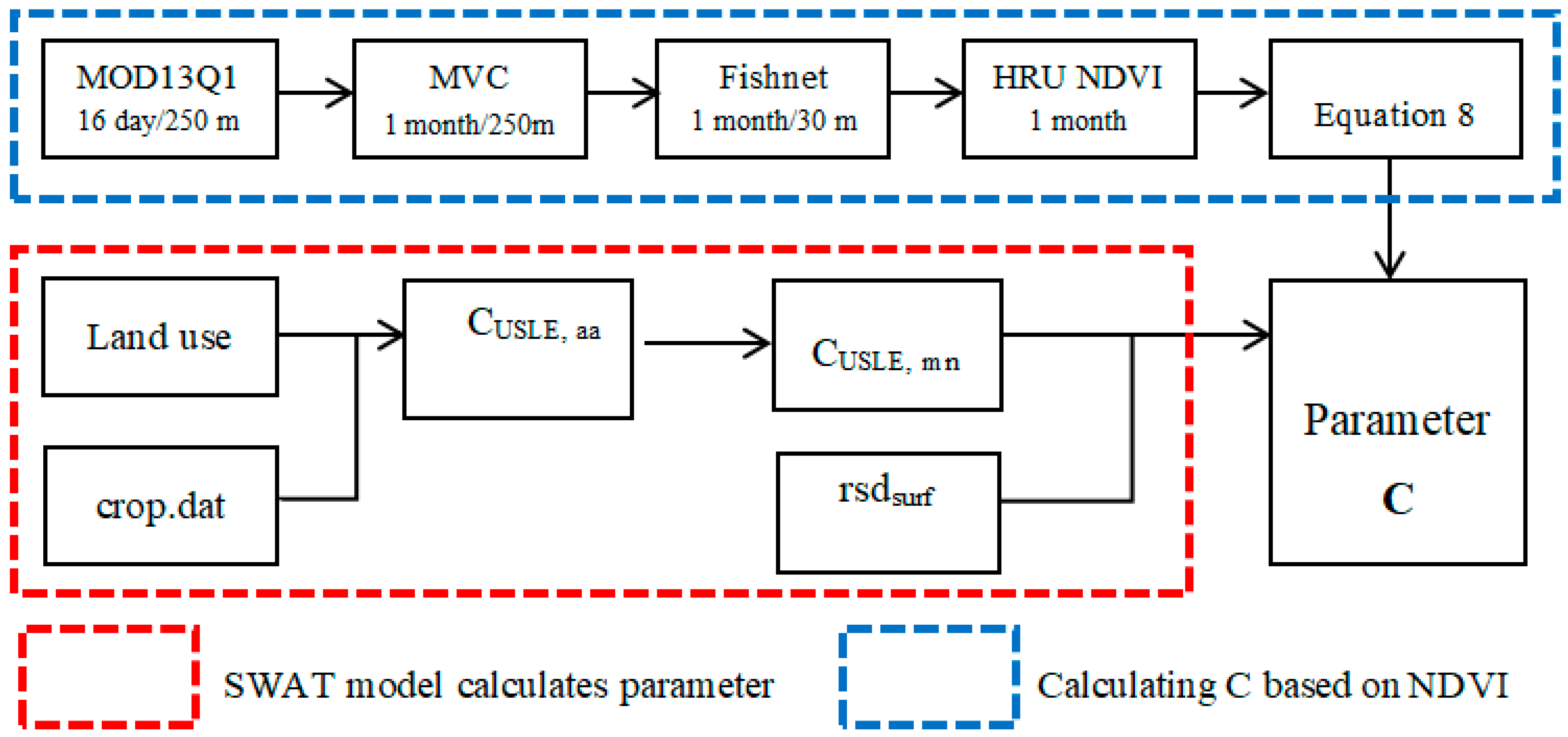
2.3.4. Integration of Remotely Sensed NDVI into SWAT

Under natural conditions, DEM and soil data vary slowly [61]; hence, these were not considered in this study. In comparison, human activity and vegetation restoration affected land use changes in the YanHe Watershed, but only one period of land use data was included in the original SWAT model.

The SWAT model reads the annual average C factor (C_USLE,aa) of a particular land use type from the crop database (crop.dat); calculates the minimum C factor (C_USLE,mn) of this land use; and calculates C_USLE based on C_USLE,mn, and soil surface residue (rsd_surf). In the long-term series simulation, the original model does not consider the impact of land use transfer on vegetation coverage changes and has some other limitations. Therefore, the study proposed recalculating C_USLE using the remotely sensed NDVI to reflect real vegetation cover changes.

MOD13Q1 is a long-term serial product of the MODIS series, which can express vegetation changes in agricultural land in different seasons and farming modes without additional measurements or special satellite-data processing [62]. Considering the spatial resolution of the land use, soil, and slope data and the smallest unit of HRU as 30 × 30 m, we generated a 30 × 30 m fishnet based on the DEM raster map. Using the “Extract Multi Values to Points” tool provided by ArcGIS, the NDVI values were then extracted for every point and the average NDVI of each HRU was calculated to obtain the monthly NDVI dataset.

Van der Knijff [63] established the relationship between NDVI and C_USLE based on National Oceanic and Atmospheric Administration (NOAA) Advanced Very-High-Resolution Radiometer (AVHRR) data as follows:

$${\mathrm{C}}_{USLE}=\exp \left[-\alpha ·\frac{NDVI}{\beta -NDVI}\right]$$

(8)

where α and β are constants. Van Leeuwen and Sammons [64] showed that when using MODIS-NDVI data, α and β should be 2.5 and 1, respectively. Therefore, we calculated the new C_USLE value based on Equation (8), for α = 2.5 and β = 1. The SWAT source code was also modified and NDVI data were introduced. Figure 2 shows the flowchart of the C_USLE modification in the SWAT model based on the NDVI data.

2.3.5. Mann-Kendall Test

The Mann–Kendall (MK) trend test is a nonparametric test method [65] widely used for trend analysis of vegetation and hydrological series. The MK test sample does not need to conform to a certain distribution and is not affected by outliers. The τ-value in the MK test reflects the correlation between the test sequence and time, and the p-value represents the significance level of the test results. The test results were divided into seven categories according to τ- and p-values to determine the trend change (

Table 2. Trend classification in terms of p-value and τ using the Mann–Kendall (MK) trend test.

τ	p-Value	Trend Type	Trend Features
	p ≤ 0.01	3	Increased very significantly
τ > 0	0.01 < p ≤ 0.05	2	Increased significantly
	0.05 < p ≤ 0.1	1	Slightly increased
τ = 0		0	No significant change
	0.05 < p ≤ 0.1	–1	Slightly decreased
τ < 0	0.01 < p ≤ 0.05	–2	Decreased significantly
	p ≤ 0.01	–3	Decreased very significantly

).

3. Results

3.1. Spatiotemporal Variations of Vegetation Cover and Evapotranspiration

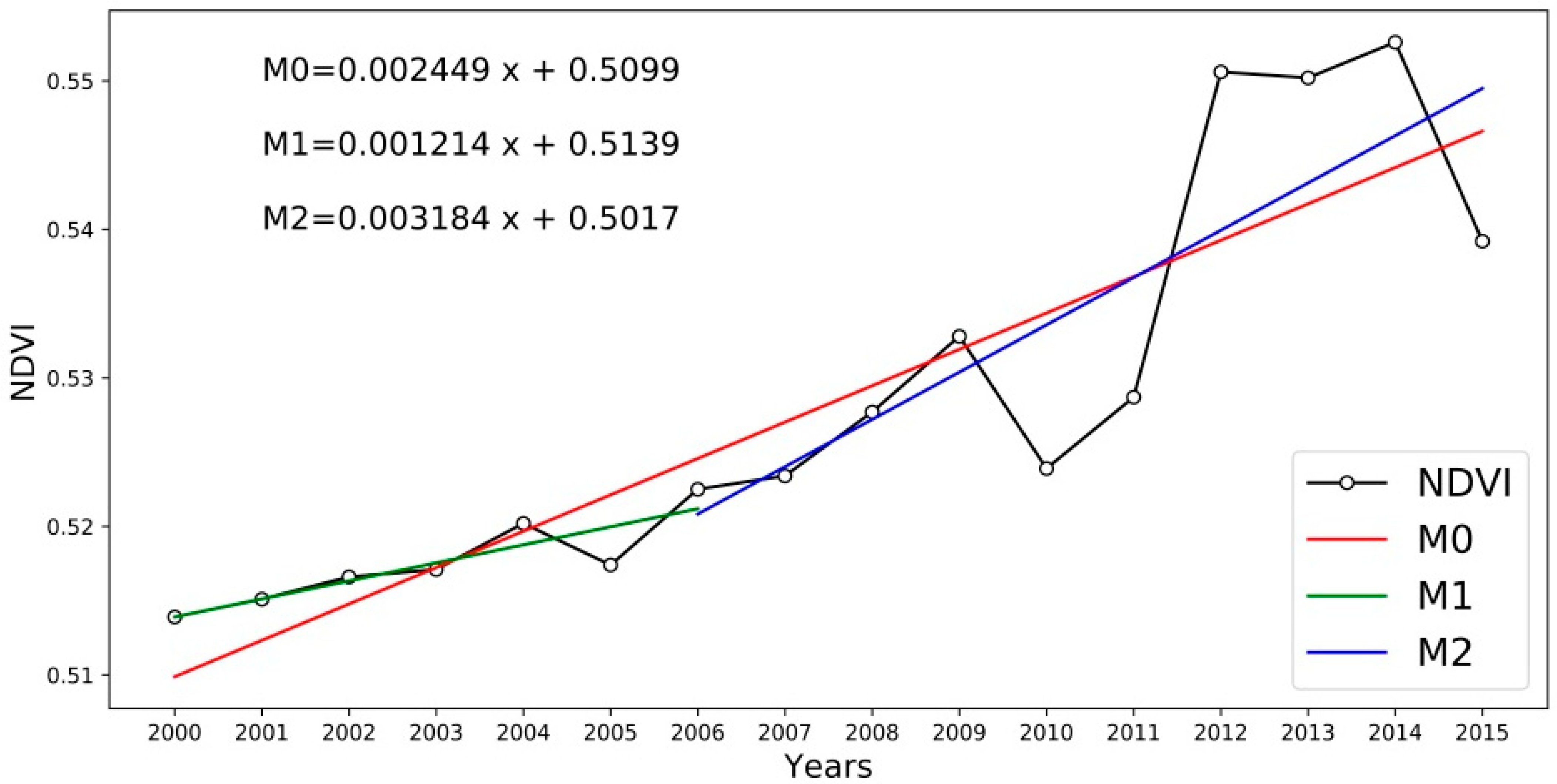
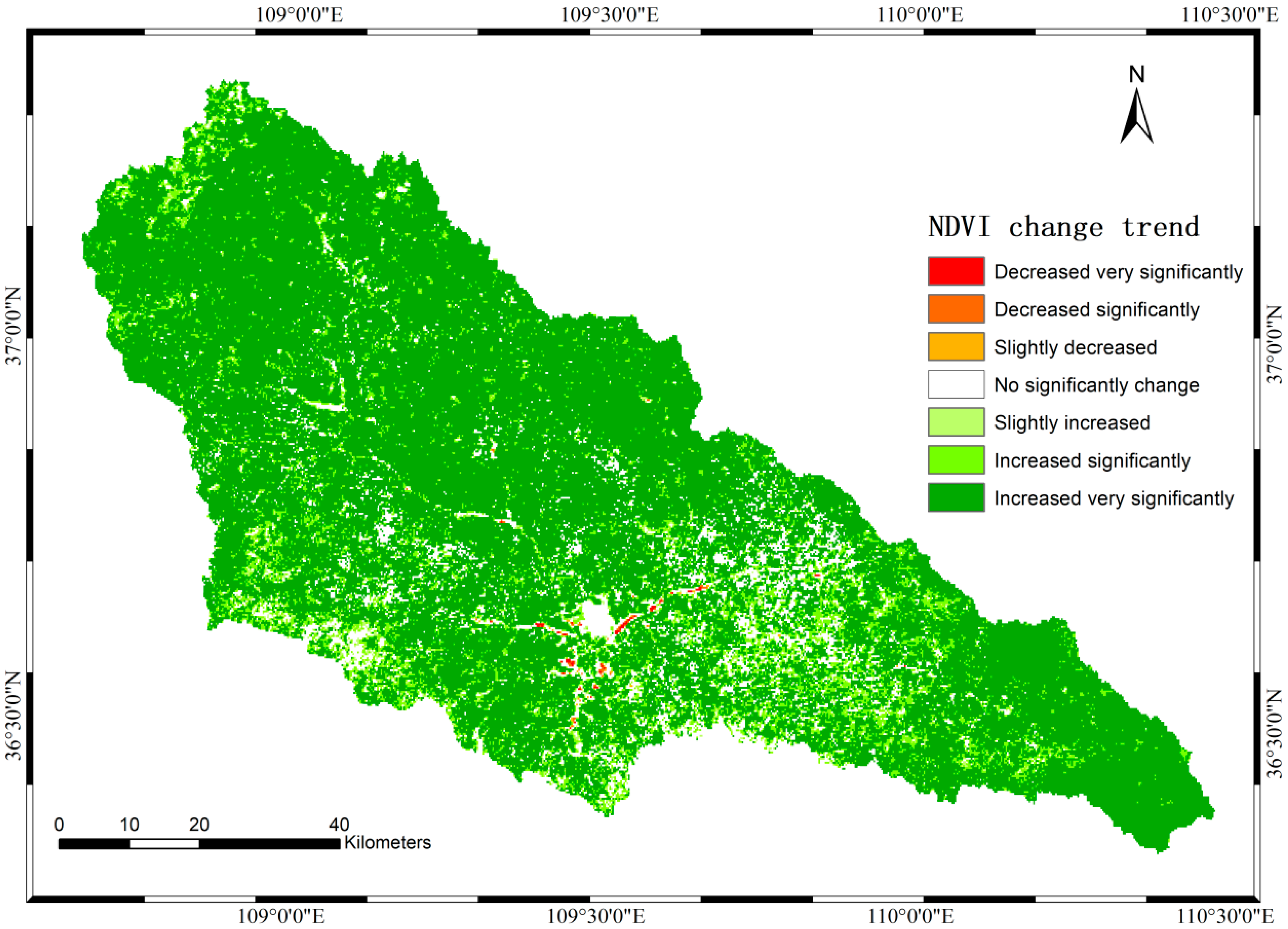
3.1.1. Changes in Vegetation Cover

The NDVI effectively monitors regional and global vegetation and is a major factor in the inversion of vegetation coverage. It is suitable for vegetation monitoring in the middle stage of vegetation development or in areas with medium vegetation cover, such as the YanHe Watershed. Several types of remote sensing techniques are utilized in such monitoring, among which MODIS NDVI has a strong temporal sequence and is available for free. Moreover, studies have shown that MODIS NDVI is more suitable for indicating vegetation conditions on the Loess Plateau; therefore, it was adopted in this study. Figure 3 shows the interannual change trend of NDVI in the YanHe Watershed from 2000 to 2015, which fluctuated between 0.514 and 0.553, with a multi-year average of 0.5282. Under the influence of human factors, vegetation cover steadily increased, with an average growth rate of 0.0245 × 10a⁻¹. The ecological protection project achieved notable results. During the initial stage of the GFGP (2000–2005), vegetation cover increased at a slower rate than the average for the entire period (0.0121 × 10a⁻¹). During the middle and later periods of the GFGP (2006–2015), the NDVI increased at a rate of 0.0318 × 10a⁻¹. In the later stages, the government focused primarily on protecting vegetation from damage. Natural environmental factors played a significant role in vegetation growth in the YanHe Watershed, resulting in a slight decrease in NDVI values in some years (2010 and 2015).

The MK trend of NDVI represents the spatial distribution of vegetation change in the YanHe Watershed during 2000–2015 (Figure 4). After commencing the GFGP, vegetation followed a significant growth trend in most parts of the YanHe Watershed, with extremely significant and significant increases accounting for 78.08% and 11.87% of the total area, respectively. Areas with noticeable vegetation growth were distributed primarily in the upstream and downstream areas of the YanHe River. The upper reaches of the river are characterized by complex topography, with steep slopes (>25°) accounting for more than 70% of the area [66], which has the most severe soil erosion in the whole basin and is a key area for the implementation of the GFGP. Thus, the vegetation cover in this area improved significantly. In the downstream area, agricultural activities were frequent; vegetation cover was poor at the start of the study; however, it was well restored after the implementation of the GFGP. In the middle reaches before the GFGP, the vegetation was relatively dense and had not changed significantly since 2000. The regions with significant vegetation degradation accounted for less than 1% of the total watershed area and were primarily distributed in the urban areas of Yan’an City. During urbanization, land use types are transformed from agricultural land and grassland to construction land, resulting in vegetation destruction and a declining NDVI trend. In general, after implementing the GFGP, the NDVI in the study area exhibited a steady increasing trend, indicating that the vegetation status of the YanHe Watershed, along with the ecological environment, had overall improved over time.

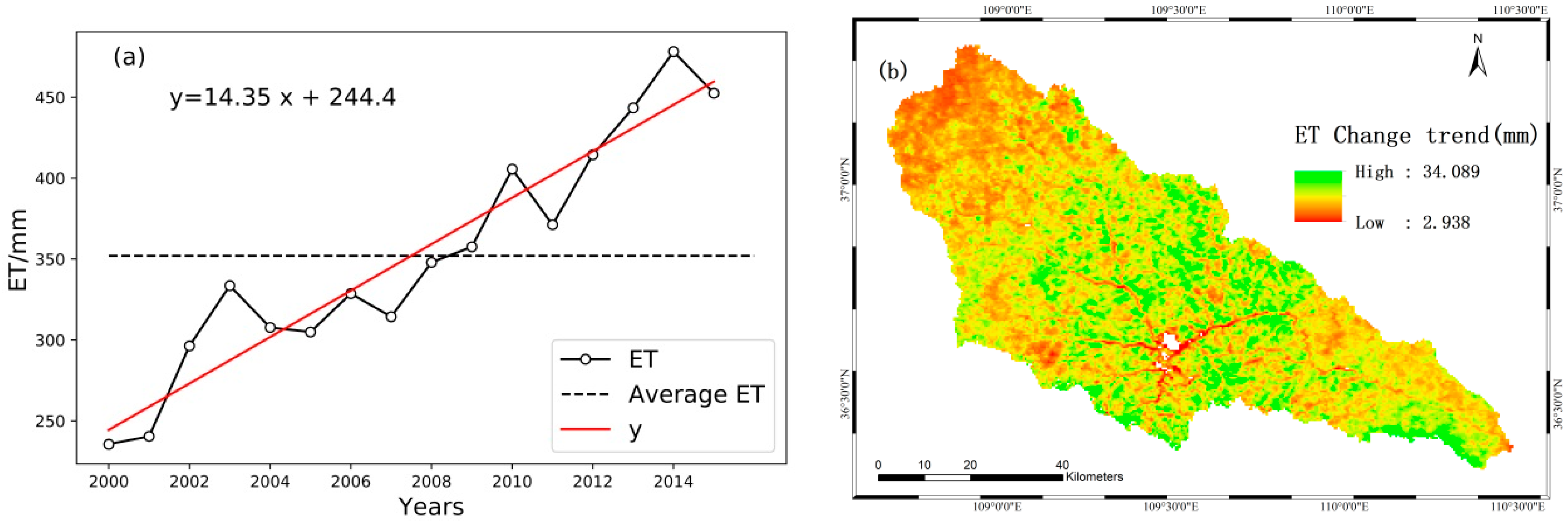
3.1.2. Changes in Evapotranspiration

Figure 5a shows the interannual variation trend of ET in the YanHe Watershed from 2000 to 2015. Annual average value of ET fluctuated between 235.55 and 478.19 mm·a⁻¹, and the multi-year average value of ET was 352.01 mm·a⁻¹ (dotted line in Figure 5a). The ET followed a significant growth trend of 14.35 mm·a⁻¹. The annual average ET was the lowest (235.55 mm·a⁻¹) in 2000 and the highest (478.19 mm·a⁻¹) in 2014. However, the annual average values of ET in 2004, 2007, 2011, and 2015 were slightly lower than those in the corresponding previous years. In general, the changing trend of ET in the YanHe Watershed was consistent with the overall change in vegetation, indicating that the GFGP affected regional vegetation growth and the hydrological cycle process and had a significant impact on terrestrial ET.

The results in Figure 5b show the MK trend in the spatial distribution of ET in the YanHe Watershed from 2000 to 2015. ET in the watershed had increased significantly during the 15 years (2000–2015) (except for a few areas with significance <95%), with noticeable regional differences. Because of the fertile soil, adequate water sources, flat terrain, and frequent human activities, vegetation cover near the river was relatively stable since 2000, and ET increased slowly. As urbanization restricted the area around Yan’an New City, vegetation restoration was not apparent, and ET remained almost unchanged. The increase in ET in the northern part of the basin was slightly higher than that near the river. Agricultural land and grassland were widely distributed in this area, but an increase in ET was not evident due to limited water availability and heat conditions, and limited changes in vegetation coverage. Adequate water and heat conditions are suitable for vegetation growth; therefore, a medium increase in ET was widely distributed in this region, with scattered areas of significant ET increase.

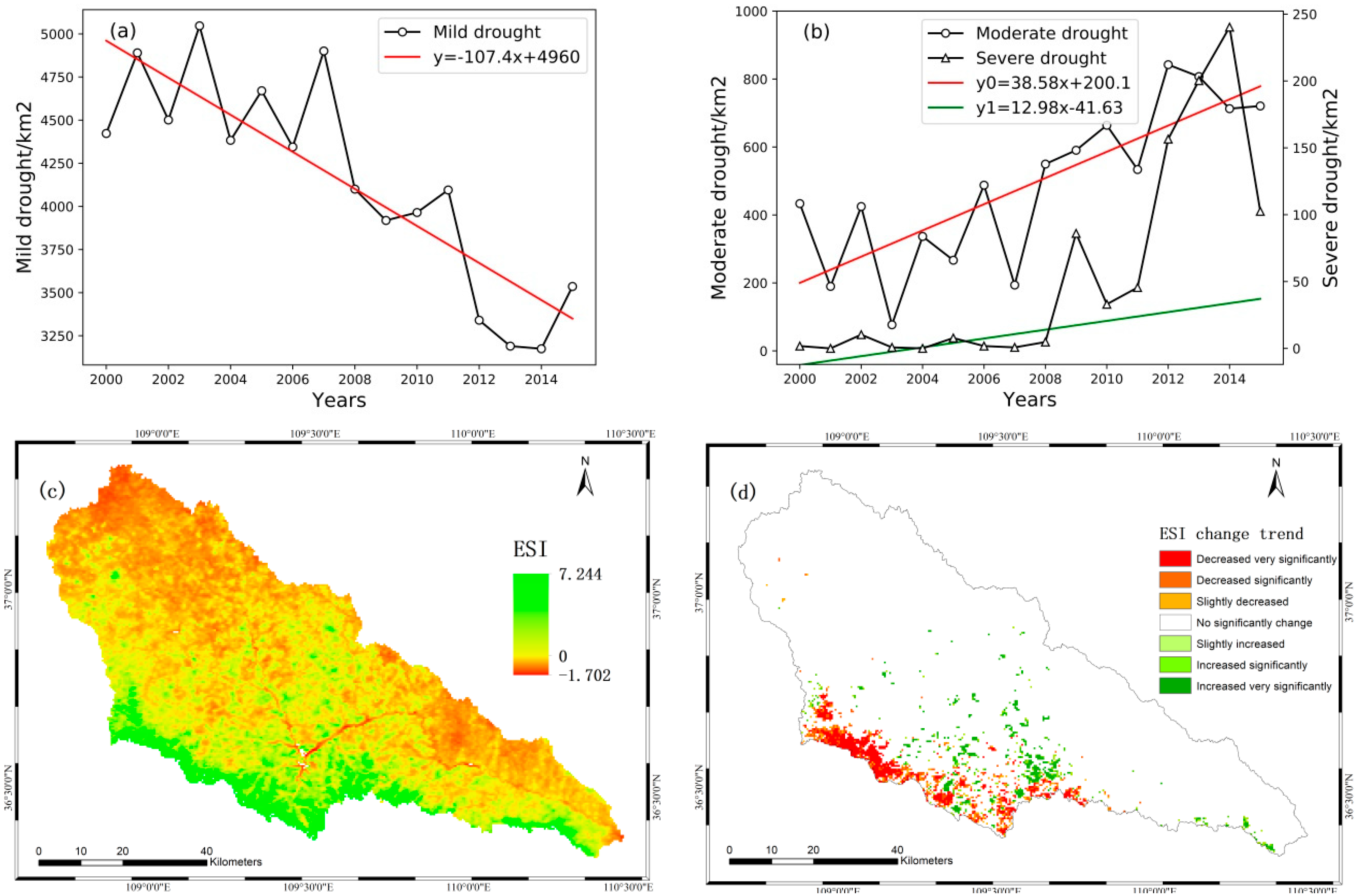
3.2. Drought Assessment Based on ESI

The variation trends of different drought levels in the YanHe Watershed from 2000 to 2015 are shown in Figure 6a,b. The mild drought area declined significantly, reaching 107.4 km²·a⁻¹. From 2000 to 2007, the proportion of mild drought fluctuated, with no apparent increasing or decreasing trend during the early growth and development of the vegetation. The area of mild drought continued to decline during 2007–2014, rebounding slightly in 2015 due to the increasing impact of vegetation restoration on the regional water balance during the later stage of the GFGP. In contrast, the moderate and severe drought areas fluctuated upward, with rates of 38.58 km²·a⁻¹ and 12.98 km²·a⁻¹, respectively. From 2000 to 2015, the YanHe Watershed experienced a significant decrease in mild drought and increases in no drought (normal level), moderate drought, and severe drought conditions. A significant regional difference was observed between dry and wet conditions, indicating a serious imbalance between water supply and demand, which should be focused upon by the government and relevant departments.

The spatial distribution map of the average ESI from 2000 to 2015 represents the degree of drought in the YanHe Watershed (Figure 6c). The arid region accounts for 63.86% of the total area, of which mild, moderate, and severe droughts accounted for 60.52%, 3.30%, and 0.04%, respectively. Comparing Figure 5b and Figure 6c, the distribution pattern of the average ESI was found to be similar to the average ET over time, indicating that the degree and distribution of drought were significantly affected by ET. In Figure 6c, the positive ESI areas (green) are concentrated in the southern edge of the basin and scattered in the middle reaches, indicating a humid climate, and small impact of drought. The negative ESI area (orange-red) is widely distributed in the upper reaches of the YanHe River, indicating severe drought; it is also slightly distributed in the lower reaches of the basin, however, the degree of drought is low. This study is based on a pixel-by-pixel calculation of ESI based on remote-sensing MODIS products. By analyzing the spatial distribution of ESI results, the spatial variation characteristics of drought can be explored in detail, which help formulate the drought prevention measures.

Figure 6d shows the MK trend in the spatial distribution of ESI in the YanHe Watershed from 2000 to 2015. Areas with significantly worse droughts were concentrated in the southwest of the basin. The main vegetation types in this area included forest and grassland with severe ET, which accelerated the loss of water resources leading to dry conditions. In summary, it was observed that vegetation restoration aggravates drought, particularly in relatively humid areas with high vegetation coverage, which may negatively affect the balance of surface water, groundwater, and soil water storage. A continuation of this phenomenon could adversely affect the quality of forestry ecological projects and the impact of the GFGP.

3.3. Soil Conservation Services Simulation and Spatiotemporal Characteristics

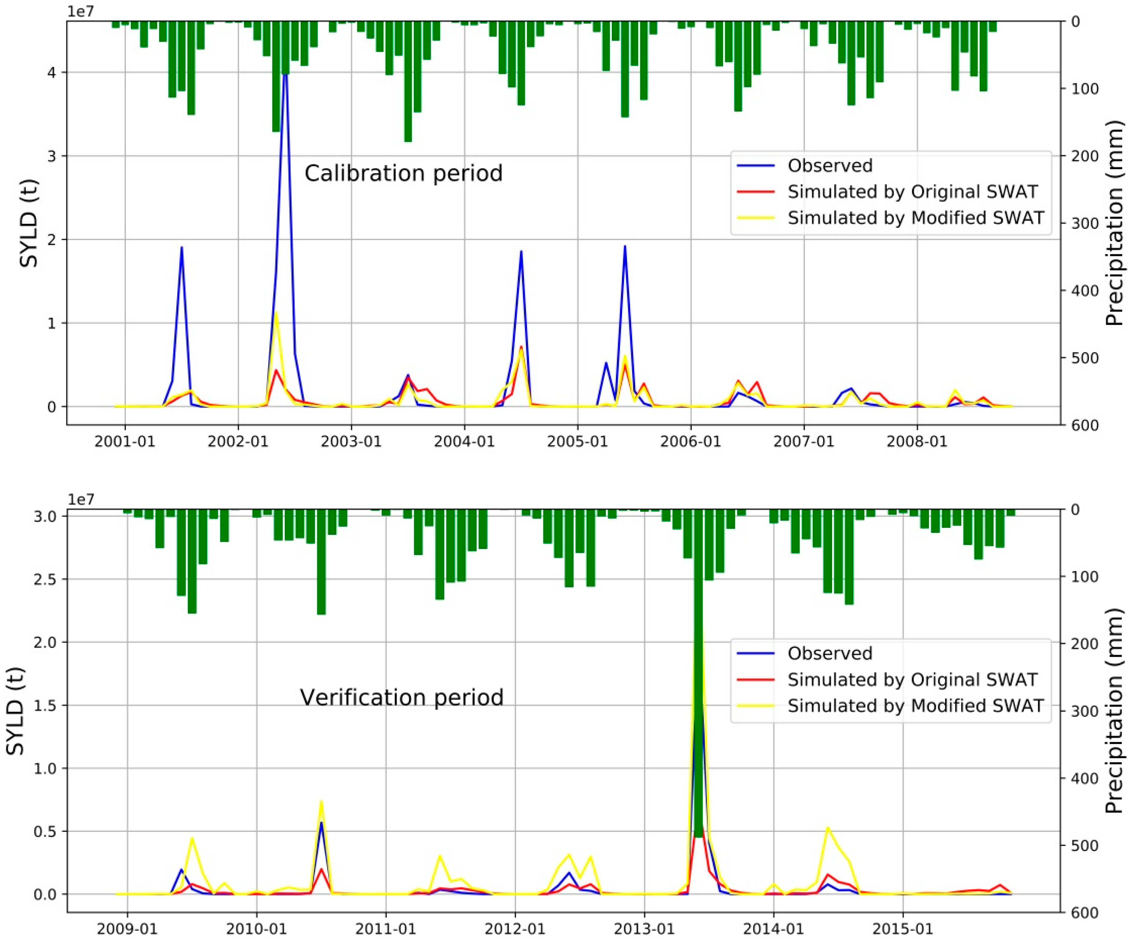
3.3.1. Evaluation and Calibration of the Modified SWAT

In this study, soil conservation in the YanHe Watershed was simulated using the modified SWAT model (Figure 7). The validation process involved input of the parameter values determined during the calibration process into the model. The simulation results for the YanHe Watershed improved during the calibration (R² and NSE increased from 0.63 to 0.76 and 0.46 to 0.51, respectively) and verification periods (R² and NSE increased from 0.82 to 0.93 and 0.57 to 0.61, respectively). After introducing the remote-sensing data, the SWAT sediment simulation increased the R², NSE, and the model simulation accuracy. During the calibration and verification periods, the monthly simulated value of sediment was consistent with the observed value and the modified model simulation result was closer to the observed value with a higher degree of correlation than that of the original model. In the study period, R² > 0.5 and NSE > 0.5 were achieved in the simulation results. Therefore, the modified SWAT model would be suitable for simulating sediment transport in the YanHe Watershed.

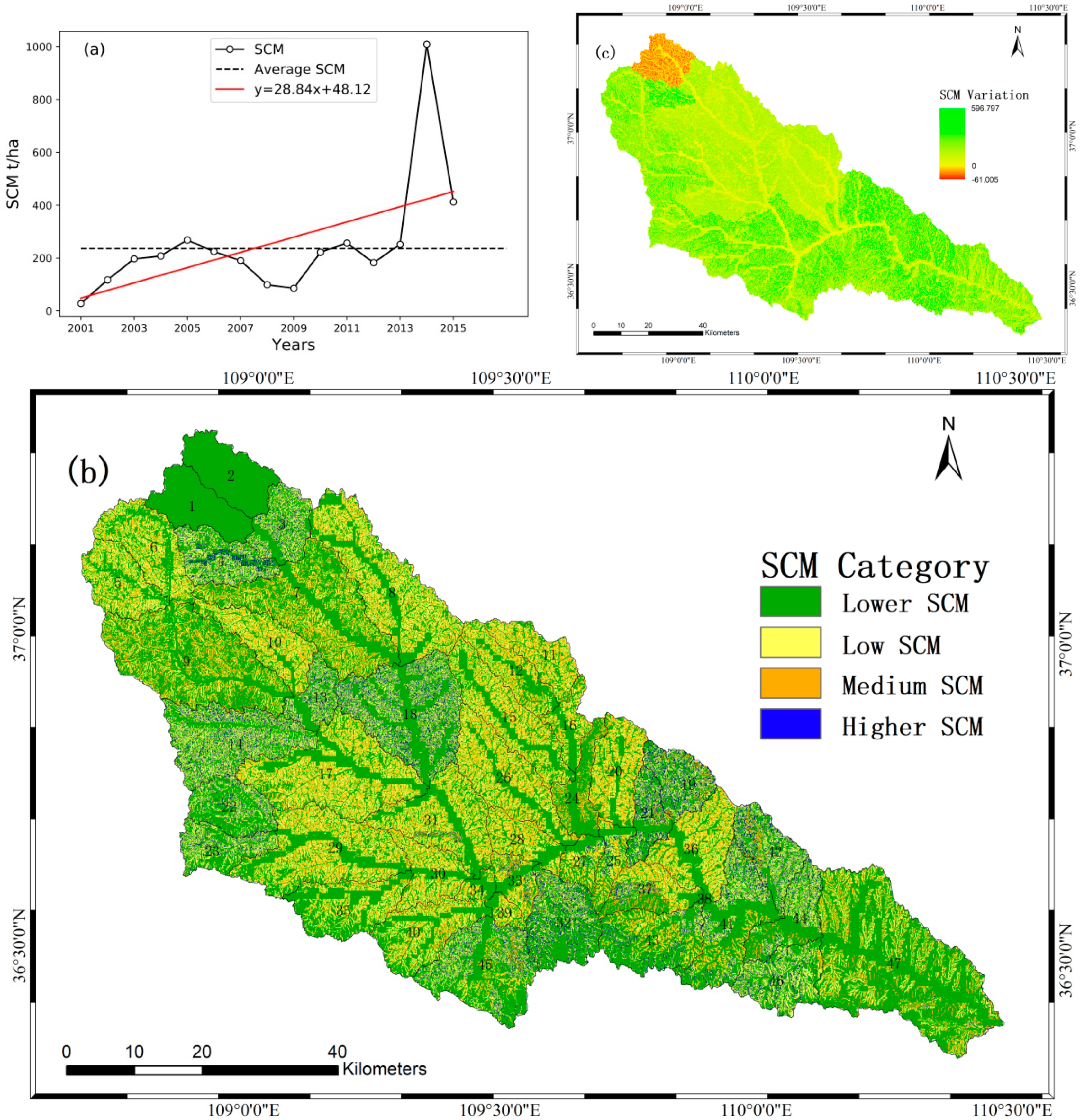
3.3.2. Spatiotemporal Variations of Soil Conservation Services

Figure 8a shows the annual average SCM time series of the YanHe Watershed during 2000–2015, which exhibited a varying and increasing trend, with a growth rate of 28.84 t·ha⁻¹·a⁻¹ and multi-year average of 235.69 t·ha⁻¹·a⁻¹ (dotted line in Figure 8a). The SCMs for 2001, 2005, 2010, and 2015 were 116.87, 224.20, 256.63, and 412.58 t·ha⁻¹·a⁻¹, respectively. From 2001 to 2005, SCM exhibited a steady growth trend as the vegetation in the watershed gradually recovered, sediment flux decreased, and soil erosion was controlled in the early stage of the GFGP. The climatic conditions during this period were relatively stable, with no extreme weather events. From 2006–2010, SCM first decreased and then increased as the GFGP process slowed and increases in vegetation were negligible. Compared to the previous period, the influence of vegetation factors decreased, and that of meteorological factors increased. Precipitation in 2008 and 2009 reduced the potential soil erosion and decreased SCM; however, it remained higher than that during the early stage of the GFGP. In the late stage of the GFGP (2011–2015), the government focused primarily on protecting the vegetation from destruction; hence, vegetation changes were not significant and the variations in SCM were primarily affected by meteorological conditions. As precipitation significantly varies the potential soil retention modulus, the SCM followed a trend consistent with the annual precipitation, particularly in 2013 (1009.03 t·ha⁻¹·a⁻¹).

Figure 8b shows the distribution pattern of SCM levels in the YanHe Watershed from 2000 to 2015, with significant spatial variations. The lower SCM accounted for 55.08% of the total area, most of which was located on both banks of the river, and the rest scattered on agricultural land. The soil erodibility factor (K) around the YanHe River was large; the erosion was severe and not conducive to the implementation of engineering measures. The surface soil activity of agricultural land was frequent because of human activities. In spring and winter, agricultural land was mostly without vegetation cover, with limited soil conservation functions. The low SCM accounted for 29.67% of the total area, which was concentrated at the bottom of the slope, with a low slope and undulating topography. The primary land use type was grassland, and the topography and surface cover of this area were relatively stable. The medium and high SCM had strong soil conservation functions, but their proportions were relatively small (10.47% and 4.78%, respectively). Most of them were located in the middle and lower reaches of the YanHe River because of the flat terrain, thick soil layer, and adequate water and heat conditions. The soil was not easily eroded, and acceptable vegetation and maintenance measures had been implemented. In contrast, soil erosion in the upper reaches was severe and not conducive to vegetation restoration because of the deep valleys, broken ground surface, and steep slopes (>25°). A high SCM was distributed in certain individual years. To reflect the average level of the soil retention function in the entire watershed, the high SCM was smoothed when calculating the multi-year average SCM.

Figure 8c shows the varying trend of the SCM in the YanHe Watershed. To reduce the impact of extreme climatic conditions, the variations in SCM during the late stage of the GFGP (2011–2015) over those during the early stage (2001–2005), were used to analyze the spatial trend in SCM. Soil conservation services in most areas of the YanHe River Basin have been increasing. The middle and lower reaches of the YanHe River are suitable for vegetation growth and ecological engineering development, which are important supply areas for soil conservation services in the basin. The upstream was found to be the key area of successful GFGP implementation, where soil erosion has been curbed and soil conservation functions have been enhanced. However, an increase in the supply of soil conservation services near the river was not apparent.

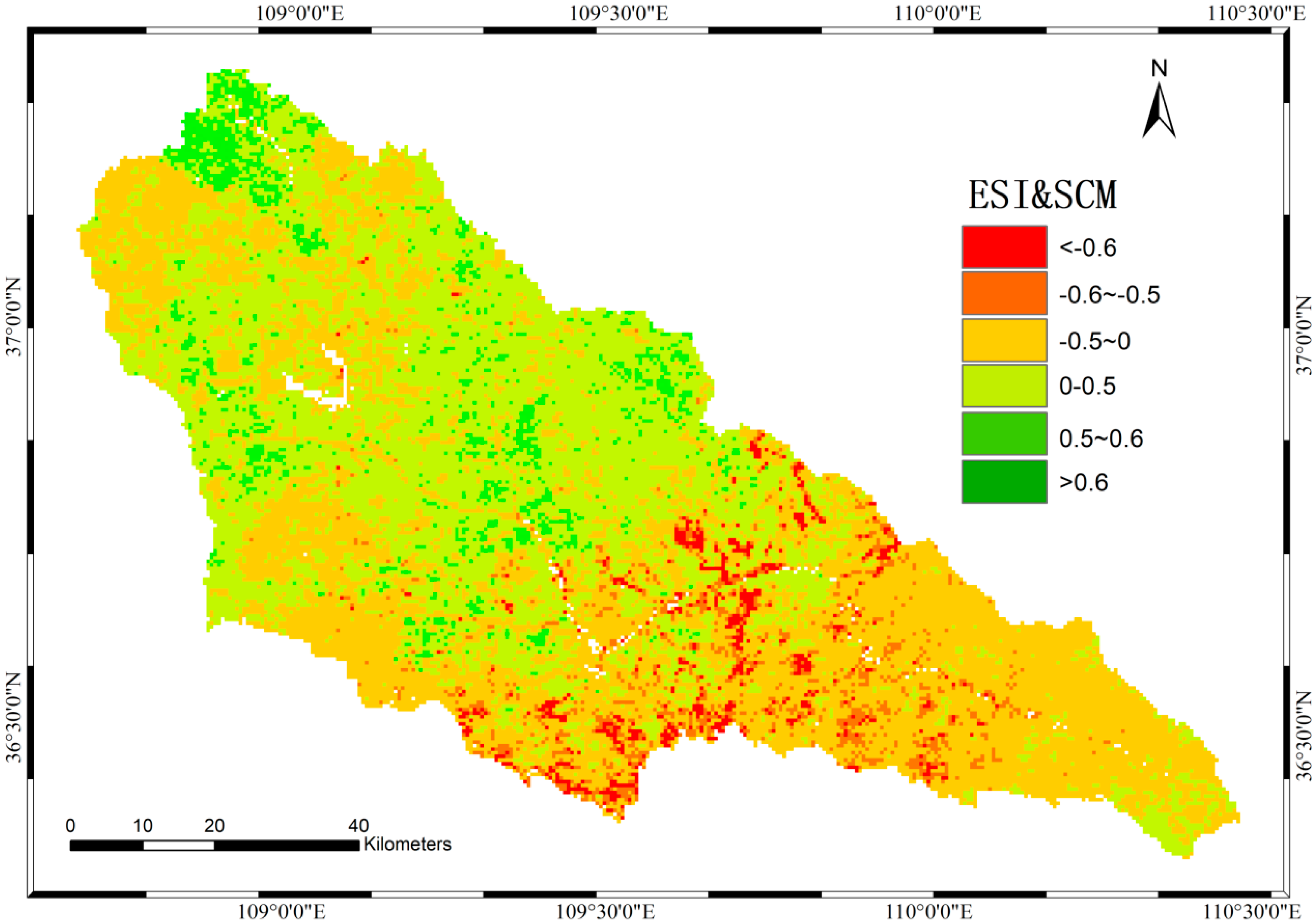
3.4. Coupling Analysis of Soil Conservation Services and Drought

Since 2000, soil conservation services and drought conditions in the YanHe Watershed have been constantly changing under the influence of vegetation restoration. Based on the monthly data of ESI, NDVI, precipitation (PCP), relative humidity (RH), wind speed (WIND), and temperature (TEM), the GRA method was adopted to evaluate the correlation between soil conservation services, drought, and other factors. The analysis results are presented in

Table 3. Connectivity between related factors and soil conservation services.

RESI	RNVDI	RPCP	RRH	RWIND	RTEM
0.9779	0.9766	0.9714	0.9552	0.7515	0.7273

. The correlation sequence of soil conservation services and related factors (was R_ESI > R_NVDI > R_PCP > R_RH > R_WIND > R_TEM, which showed that, among many factors, soil conservation services had the highest correlation with ESI, followed by NDVI and precipitation, and the least correlation with temperature.

Based on the GRA, the correlation between the SCM and ESI in the YanHe Watershed was analyzed on a spatial scale; the distribution of the spatial correlation coefficients between them are shown in Figure 9. The areas with negatively correlated SCM and ESI (red) are primarily distributed in the middle and lower reaches of the YanHe River, and the enhancement of soil conservation services in these regions was accompanied by the intensification of drought. Areas with a highly negative correlation (<−0.5) were scattered in the regions with high vegetation coverage. Vegetation can reduce the effect of raindrops, thereby reducing rainwater splash erosion; reduce the peak of floods; delay surface runoff; and reduce surface erosion by water; which effectively curbs watershed soil erosion and enhances soil conservation functions. However, the plant canopy intercepts rainfall and reduces the amount of water that reaches the ground. Vegetation restoration increases transpiration and biomass, resulting in increased surface crust and reduced infiltration. These factors lead to a decrease in groundwater recharge, an increase in water consumption from deep groundwater, a decrease in soil water content, and an aggravation of regional drought. The areas where SCM and ESI are positively correlated (green) are scattered in the upper reaches of the YanHe River, occupying a small proportion. Drought in these areas has been alleviated by the enhancement of soil conservation services. Because of the differences in vegetation types, topography, climate, and other factors, the correlation between soil conservation services and drought exhibited spatial variations.

4. Discussion

This study focused on drought and soil conservation services to evaluate the ecological effects of vegetation restoration in the YanHe Watershed. Using remote sensing data, this study analyzed spatiotemporal variations in vegetation cover and ET in the watershed. To meet the requirements of the study period and analyze data on a spatial scale, this study utilized currently available MODIS products. The results of this study are consistent with other studies: The GRGP significantly increased vegetation cover in the YanHe River Basin, and the large-scale restoration of vegetation [67,68] has been accompanied by a significant increase in regional ET and water consumption [69]. This study used ESI to characterize the degree of drought in the basin and evaluate the response of drought to the increase in ET. Compared to SPI and SPEI, the ESI accounted for the role of ET in the evolution of drought, which can better reflect the response of vegetation and soil moisture to drought [70], although it did not consider the impact of meteorological factors (precipitation) on drought. Herein, soil conservation services in the YanHe Watershed were simulated, based on the modified SWAT model which was integrated with remote sensing data. The original SWAT model calculates the C-factor based on land use data, which does not accurately express the variation in vegetation cover. The study recalculated C_USLE using a remotely sensed NDVI value to better reflect real vegetation cover changes when simulating soil conservation. The limitations of this study include: (1) Because of limited availability of remote sensing data sources, the modified SWAT did not integrate NDVI data with high temporal and spatial resolutions; however, the simulation accuracy was higher than that of the original model; (2) there is a lack of research on value accounting of ESs, which plays a limited role in the ecological compensation field of the basin. Further research should be conducted to consider the impact of climate change and human activities, analyze the relationship between drought and ESs from the perspective of physical mechanisms, and evaluate the value of ESs to guide eco-compensation.

5. Conclusions

The main findings of the study are as follows:

• GRA has significant advantages in studying the factors affecting ESs. Soil conservation services in the YanHe Watershed are closely related to ESI and NDVI, followed by rainfall. Spatial variations exist in the correlations between soil conservation services and drought. In the middle and lower reaches of the YanHe River, drought in the regions covered by vegetation was aggravated with the enhancement of soil conservation services. The drought in parts of the mountainous area in the upper reaches of the YanHe River decreased with the enhancement of soil conservation services.
• From 2000 to 2015, with the implementation of the GFGP, vegetation status significantly improved, but plant water consumption increased with increasing ET. The average annual growth rate of NDVI in the entire basin was 0.0245 × 10a⁻¹, whereas the growth rate of ET was 14.35 mm·a⁻¹.
• Arid regions in the YanHe Watershed accounted for 63.86% of the total area, and the spatial distribution of drought increased from south to north. From 2000 to 2015, the overall distribution pattern of wet and dry conditions in the basin varied negligibly. Drought in parts of the midstream area of the YanHe River has been alleviated, while the humid regions have become drier.
• Vegetation restoration can effectively weaken soil erosion and improve the soil conservation functions of ecosystems. The SCM increased from 116.87 t·ha⁻¹·a⁻¹ (2000) to 412.58 t·ha⁻¹·a⁻¹ (2015), indicating a steady growth trend of 28.84 t·ha⁻¹·a⁻¹.
• The integration of remote sensing NDVI into SWAT enabled the fusion of remote sensing and non-remote sensing data, which enhanced the reliability of the original model and improved simulation accuracy.

Considering the water conservation and supply of soil conservation services, vegetation restoration in the YanHe Watershed should incorporate low-water-consumption tree species and restrict density of afforestation. The study results will help in evaluating the ecological effects of the GFGP and provide valuable information for formulating ecological policies on the Loess Plateau thereby enabling sustainable development of the ecosystem.

References

1. Daily, G.C. Nature’s Services: Societal Dependence on Natural Ecosystems; Island Press: Washington, DC, USA, 1997. [Google Scholar]
2. Liu, Y.; Zhao, W.W.; Jia, L.Z. Soil conservation service: Concept, assessment, and outlook. Acta Ecol. Sin. 2019, 39, 432–440. (In Chinese) [Google Scholar]
3. Yang, X.M.; Wang, F.; Bento, C.P.M.; Xue, S.; Gai, L.T.; Dam, R.V.; Mol, H.; Ritsema, C.J.; Geissen, V. Short-term transport of glyphosate with erosion in Chinese loess soil—A flume experiment. Sci. Total Environ. 2015, 512–513, 406–414. [Google Scholar] [CrossRef] [PubMed]
4. Wang, F.; Mu, X.M.; Li, R.; Fleskens, L.; Stringer, L.C.; Ritsema, C.J. Co-evolution of soil and water conservation policy and human-environment linkages in the Yellow River Basin since 1949. Sci. Total Environ. 2015, 508, 166–177. [Google Scholar] [CrossRef] [PubMed] [Green Version]
5. Allen, C.D.; Macalady, A.K.; Chenchouni, H.; Bachelet, D.; McDowell, N.; Vennetier, M.; Kitzberger, T.; Rigling, A.; Breshears, D.D.; Hogg, E.H.; et al. A global overview of drought and heat-induced tree mortality reveals emerging climate change risks for forests. For. Ecol. Manag. 2009, 259, 660–684. [Google Scholar] [CrossRef] [Green Version]
6. Bennett, A.C.; McDowell, N.G.; Allen, C.D.; Anderson-Teixeira, K.J. Larger trees suffer most during drought in forests worldwide. Nat. Plants 2015, 1, 1–5. [Google Scholar] [CrossRef] [PubMed]
7. Yao, N.; Li, Y.; Lei, T.J.; Peng, L.L. Drought evolution, severity and trends in mainland China over 1961–2013. Sci. Total Environ. 2018, 616, 73–89. [Google Scholar] [CrossRef]
8. Dai, A. Increasing drought under global warming in observations and models. Nat. Clim. Chang. 2013, 3, 52–58. [Google Scholar] [CrossRef]
9. Zhang, Z.X.; Chen, X.; Xu, C.Y.; Hong, Y.; Hardy, J.; Sun, Z.H. Examining the influence of river–lake interaction on the drought and water resources in the Poyang Lake basin. J. Hydrol. 2015, 522, 510–521. [Google Scholar] [CrossRef]
10. Lesk, C.; Rowhani, P.; Ramankutty, N. Influence of extreme weather disasters on global crop production. Nature 2016, 529, 84–87. [Google Scholar] [CrossRef]
11. Stagge, J.H.; Kohn, I.; Tallaksen, L.M.; Stahl, S. Modeling drought impact occurrence based on meteorological drought indices in Europe. J. Hydrol. 2015, 530, 37–50. [Google Scholar] [CrossRef]
12. Guo, Z.L.; Huang, N.; Dong, Z.B.; Van Pelt, R.; Zobeck, T. Wind Erosion Induced Soil Degradation in Northern China: Status, Measures and Perspective. Sustain. Basel. 2014, 6, 8951–8966. [Google Scholar] [CrossRef] [Green Version]
13. Kagabo, D.M.; Stroosnijder, L.; Visser, S.M.; Moore, D. Soil erosion, soil fertility and crop yield on slow-forming terraces in the highlands of Buberuka, Rwand. Soil Tillage Res. 2013, 128, 23–29. [Google Scholar] [CrossRef]
14. Rienzi, E.A.; Fox, J.F.; Grove, J.H.; Matocha, C.J. Interrill erosion in soils with different land uses: The kinetic energy wetting effect on temporal particle size distribution. Catena 2013, 107, 130–138. [Google Scholar] [CrossRef]
15. Krasa, J.; Dostal, T.; Jachymova, B.; Bauer, M.; Devaty, J. Soil erosion as a source of sediment and phosphorus in rivers and reservoirs-watershed analyses using WaTEM/SEDEM. Environ. Res. 2019, 171, 470–483. [Google Scholar] [CrossRef] [PubMed]
16. Shi, Z.H.; Wang, L.; Liu, Q.J. Soil Erosion: From Comprehensive Control to Ecological Regulation. Bull. Chin. Acad. Sci. 2018, 33, 198–205. (In Chinese) [Google Scholar]
17. Li, Z.Y.; Fang, H.Y. Impacts of climate change on water erosion: A review. Earth Sci. Rev. 2016, 163, 94–117. [Google Scholar] [CrossRef]
18. Gao, J.L.; Zhang, J.G.; Zhu, L.L.; Ma, H.B.; Su, P.F.; Li, X. Change Characteristics of Key Measures of Soil and Water Conservation in Hill-gully Region of Loess Plateau. Bull. Soil Water Conserv. 2019, 39, 114–118. (In Chinese) [Google Scholar]
19. Zhang, H.Y.; Fang, N.F.; Shi, Z.H. Spatio-temporal patterns for the NDVI and its responses to climatic factors in the Loess Plateau, China. Acta Ecol. Sin. 2016, 36, 3960–3968. (In Chinese) [Google Scholar]
20. Zhang, B.Q.; Wu, P.T.; Zhao, X.N. Detecting and analysis of spatial and temporal variation of vegetation cover in the Loess Plateau during 1982–2009. Trans. Chin. Soc. Agric. Eng. 2011, 27, 287–293. (In Chinese) [Google Scholar]
21. Zhao, X.; Wu, P.; Gao, X.; Persaud, N. Soil quality indicators in relation to land use and topography in a small catchment on the Loess Plateau of China. Land Degrad. Dev. 2015, 26, 54–61. [Google Scholar] [CrossRef]
22. Bullock, A.; King, B. Evaluating China’s slope land conversion program as sustainable management in Tianquan and Wuqi Counties. J. Environ. Manag. 2011, 92, 1916–1922. [Google Scholar] [CrossRef] [PubMed]
23. Zhang, K.; Lu, Y.H.; Fu, B.J. Vegetation restoration and its impact on ecosystem services in typical areas of the Loess Plateau. J. Ecol. Rural Environ. 2017, 33, 23–31. (In Chinese) [Google Scholar]
24. Yang, B.; Wang, Q.J.; Xu, X.T. Evaluation of soil loss change after Grain for Green Project in the Loss Plateau: A case study of Yulin, China. Environ. Earth Sci. 2018, 77, 304. [Google Scholar] [CrossRef]
25. Léa, K.; Romain, A.; Mathieu, S.; Jean-François, O.; Michel-Pierre, F. Plant functional trait effects on runoff to design herbaceous hedges for soil erosion control. Ecol. Eng. 2018, 118, 143–151. [Google Scholar]
26. Gashaw, T.; Tulu, T.; Argaw, M.; Worqlul, A.W.; Tolessa, T.; Kindu, M. Estimating the impacts of land use/land cover changes on Ecosystem Service Values: The case of the Andassa watershed in the Upper Blue Nile basin of Ethiopia. Ecosyst. Serv. 2018, 31, 219–228. [Google Scholar] [CrossRef]
27. Tobler, W.R. Computer movie simulating urban growth in the Detroit region. Econ. Geogr. 1970, 46, 234–240. [Google Scholar] [CrossRef]
28. Shen, M.; Piao, S.; Jeong, S.J.; Zhou, L.M.; Zeng, Z.Z.; Ciais, P.; Chen, D.; Huang, M.T.; Jin, C.S.; Li, L.Z.X.; et al. Evaporative cooling over the Tibetan Plateau induced by vegetation growth. Proc. Natl. Acad. Sci. USA 2015, 112, 9299–9304. [Google Scholar] [CrossRef] [PubMed] [Green Version]
29. Cao, X.C.; Wang, Y.B.; Wu, P.T.; Zhao, X.N.; Wang, J. An evaluation of the water utilization and grain production of irrigated and rain-fed croplands in China. Sci. Total Environ. 2015, 529, 10–20. [Google Scholar] [CrossRef]
30. Shi, Y.F.; Liang, S.Q.; Peng, S.Z. Spatiotemporal Variation of Climate Drought in Loess Plateau Region during 1901–2017. Bull. Soil Water Conserv. 2020, 40, 283–289. (In Chinese) [Google Scholar]
31. Wang, Y.S.; Li, X.Y.; Shi, F.Z.; Zhang, S.L.; Wu, X.L. The Grain for Green Project intensifies evapotranspiration in the revegetation area of the Loess Plateau in China. Chin. Sci. Bull. 2019, 64 (Suppl. Z1), 588–599. (In Chinese) [Google Scholar] [CrossRef] [Green Version]
32. Ge, J.; Pitman, A.J.; Guo, W.D.; Zan, B.L.; Fu, C.B. Impact of revegetation of the Loess Plateau of China on the regional growing season water balance. Hydrol. Earth Syst. Sc. 2020, 24, 515–533. [Google Scholar] [CrossRef] [Green Version]
33. Yuan, S.S.; Quiring, S.M. Drought in the U.S. Great Plains (1980–2012): A sensitivity study using different methods for estimating potential evapotranspiration in the Palmer Drought Severity Index. J. Geophys. Res. Atmos. 2014, 119, 10996–11010. [Google Scholar] [CrossRef]
34. Vicente-Serrano, S.M.; Beguería, S.; López-Moreno, J.I. A Multiscalar Drought Index Sensitive to Global Warming: The Standardized Precipitation Evapotranspiration Index. J. Clim. 2010, 23, 1696–1710, 1712, 1714–1718. [Google Scholar] [CrossRef] [Green Version]
35. Potop, V.; Možný, M.; Soukup, J. Drought evolution at various time scales in the lowland regions and their impact on vegetable crops in the Czech Republic. Agric. For. Meteorol. 2012, 156, 121–133. [Google Scholar] [CrossRef]
36. Zhang, S.L.; Yang, D.W.; Yang, Y.T.; Piao, S.L.; Yang, H.B.; Lei, H.M.; Fu, B.J. Excessive Afforestation and Soil Drying on China’s Loess Plateau. J. Geophys. Res. Biogeo. 2018, 123, 923–935. [Google Scholar] [CrossRef]
37. Wei, X.H.; Rao, X.J.; Kong, X.Y.; Ma, H.W. Research on drought monitoring based on remote sensing data. Hubei Agric. Sci. 2016, 55, 4598–4603. (In Chinese) [Google Scholar]
38. Wang, W.; Huang, J.; Cui, W. Application comparison of drought indices in remote sensing monitoring of drought in Yunnan-Guizhou Plateau. Trans. Chin. Soc. Agric. Eng. 2018, 34, 131–139. (In Chinese) [Google Scholar]
39. Otkin, J.A.; Haigh, T.; Mucia, A.; Anderson, M.C.; Hain, C.R. Comparison of agricultural stakeholder survey results and drought monitoring datasets during the 2016 U.S. Northern Plains flash drought Weather. Climate 2018, 10, 867–883. [Google Scholar]
40. Yoon, D.H.; Nam, W.H.; Lee, H.J.; Hong, E.M.; Kim, T.; Shin, A.K.; Svoboda, M.D. Application of Evaporative Stress Index (ESI) for Satellite-based Agricultural Drought Monitoring in South Korea. J. Korean Soc. Agric. Eng. 2018, 60, 121–131. [Google Scholar]
41. Liu, Y.Q.; Hao, L.; Zhou, D.C.; Pan, C.; Liu Pl Xiong, Z.; Sun, G. Identifying a transition climate zone in an arid river basin using the evaporative stress index. Nat. Hazard. Earth Sys. Sci. 2019, 19, 2281–2294. [Google Scholar] [CrossRef] [Green Version]
42. Zhang, B.Q.; He, C.S.; Burnham, M.; Zhang, L.H. Evaluating the coupling effects of climate aridity and vegetation restoration on soil erosion over the Loess Plateau in China. Sci. Total Environ. 2016, 539, 436–449. [Google Scholar] [CrossRef] [PubMed]
43. Hains-Young, R.; Potschin, M. The links between biodiversity, ecosystem services and human well-being. In Ecosystem Ecology: A New Systhsis; Raffaelli, D., Frid, C., Eds.; Cambridge University Press: Cambridge, UK, 2010. [Google Scholar]
44. Daily, G.C.; Polasky, S.; Goldstein, J.; Kareiva, P.M.; Mooney, H.A.; Pejchar, L.; Ricketts, T.H.; Salzman, J.; Shallenberger, R. Ecosystem services in decision making: Time to deliver. Front. Ecol. Environ. 2009, 7, 21–28. [Google Scholar] [CrossRef] [Green Version]
45. Zhou, Z.X. The Coupling Analysis of Landscape Pattern and Hydrological Process in YanHe Watershed. Ph.D. Thesis, Shaanxi Normal University, Xi’an, Shaanxi, China, 2014. (In Chinese). [Google Scholar]
46. Yang, K.J.; Lu, C.H. Evaluation of land-use change effects on runoff and soil erosion of a hilly basin—The Yanhe River in the Chinese Loess Plateau. Land Degrad. Dev. 2018, 29, 1211–1221. [Google Scholar] [CrossRef]
47. Gao, P.; Jiang, G.T.; Wei, Y.P.; Mu, X.M.; Wang, F.; Zhao, G.J.; Sun, W.Y. Streamflow regimes of the Yanhe River under climate and land use change, Loess Plateau, China. Hydrol. Process. 2015, 29, 2402–2413. [Google Scholar] [CrossRef]
48. Rehman, E.; Ikram, M.; Feng, M.T.; Rehman, S. Sectoral-based CO2 emissions of Pakistan: A novel Grey Relation Analysis (GRA) approach. Environ. Sci. Pollut. R. 2020, 27, 29118–29129. [Google Scholar] [CrossRef]
49. Deng, J.L. Basic method of grey system. Huazhong Inst. Technol. Press 1987, 11, 1–24. (In Chinese) [Google Scholar]
50. Anderson, M.C.; Hain, C.; Wardlow, B.; Pimstein, A.; Mecikalski, J.R.; Kustas, W.P. Evaluation of Drought Indices Based on Thermal Remote Sensing of Evapotranspiration over the Continental United States. J. Clim. 2011, 24, 2025–2044. [Google Scholar] [CrossRef]
51. Zhou, J.; He, D.; Xie, Y.F.; Liu, Y.; Yang, Y.H.; Sheng, H.; Guo, H.C.; Zhao, L.; Zou, R. Integrated SWAT model and statistical downscaling for estimating streamflow response to climate change in the Lake Dianchi watershed, China. Stoch. Env. Res. Risk. Assess. 2015, 29, 1193–1210. [Google Scholar] [CrossRef]
52. Chen, D.S.; Li, J.; Zhou, Z.X.; Liu, Y.; Li, T.; Liu, J.Y. Simulating and mapping the spatial and seasonal effects of future climate and land -use changes on ecosystem services in the Yanhe watershed, China. Environ. Sci. Pollut. Res. 2018, 25, 1115–1131. [Google Scholar] [CrossRef]
53. Yan, R.; Zhang, X.Q.; Yan, X.J.; Zhang, J.J.; Chen, H. Spatial patterns of hydrological responses to land use/cover change in a catchment on the Loess Plateau, China. Ecol. Indic. 2018, 92, 151–160. [Google Scholar] [CrossRef]
54. Zhang, L.; Karthikeyan, R.; Bai, Z.; Srinivasan, R. Analysis of streamflow responses to climate variability and land use change in the Loess Plateau region of China. Catena 2017, 154. [Google Scholar] [CrossRef]
55. Ren, Z.P.; Feng, Z.H.; Li, P.; Wang, D.; Cheng, S.D.; Gong, J.F. Response of runoff and sediment yield from climate change in the Yanhe Watershed, China. J. Coastal. Res. 2017, 30–35. [Google Scholar] [CrossRef]
56. Abbaspour, K.C.; Rouholahnejad, E.; Vaghefi, S.; Srinivasan, R.; Yang, H.; Kløve, B. A continental-scale hydrology and water quality model for Europe: Calibration and uncertainty of a high-resolution large-scale SWAT model. J. Hydrol. 2015, 524, 733–752. [Google Scholar] [CrossRef] [Green Version]
57. Meaurio, M.; Zabaleta, A.; Uriarte, J.A.; Srinivasan, R.; Antigüedad, I. Evaluation of SWAT models performance to simulate streamflow spatial origin. The case of a small forested watershed. J. Hydrol. 2015, 525, 326–334. [Google Scholar] [CrossRef]
58. Chen, D.S.; Li, J.; Yang, X.N.; Zhou, Z.X.; Pan, Y.Q.; Li, M.C. Quantifying water provision service supply, demand and spatial flow for land use optimization: A case study in the YanHe watershed. Ecosyst. Serv. 2020, 43, 101117. [Google Scholar] [CrossRef]
59. Li, J.; Zhou, Z.X. Landscape pattern and hydrological processes in YanHe River basin of China. Acta Geogr. Sin. 2014, 69, 933–944. (In Chinese) [Google Scholar]
60. Jiang, C.L.; Zhang, L.J.; Zhang, H.W.; Jiang, C.Y.; Yu, Y.; Pan, T. Quantitative evaluation of soil conservation in 2000–2010 in Heilongjiang Province using RUSLE model. Chin. J. Eco Agric. 2015, 23, 642–649. (In Chinese) [Google Scholar]
61. Liu, J.M.; Yuan, D.; Zhang, L.P.; Zou, X.; Song, X.Y.; Gelfan, A. Comparison of Three Statistical Downscaling Methods and Ensemble Downscaling Method Based on Bayesian Model Averaging in Upper Hanjiang River Basin, China. Adv. Meteorol. 2015, 2016. [Google Scholar] [CrossRef]
62. Ma, T.X.; Duan, Z.; Li, R.K.; Song, X.F. Enhancing SWAT with remotely sensed LAI for improved modelling of ecohydrological process in subtropic. J. Hydrol. 2019, 570, 802–815. [Google Scholar] [CrossRef] [Green Version]
63. Van der Knijff, J.M.; Jones, R.J.A.; Montanarella, L. Soil Erosion Risk Assessment in Europe; EUR 19044 EN; Office for Publications of the European Communities: Luxembourg, 2000. [Google Scholar]
64. Van Leeuwen, W.J.D.; Sammons, G. Vegetation dynamics and erosion modeling using remotely sensed data (MODIS) and GIS. In Proceedings of the Tenth Biennial USDA Forest Service Remote Sensing Applications Conference, Salt Lake City, UT, USA, 5–9 April 2004. [Google Scholar]
65. Mann, H.B. Nonparametric tests against trend. Econometrica 1945, 13, 245259. [Google Scholar] [CrossRef]
66. Wang, Z.J. Research on the Characteristics of Vegetation and Erosion and Sediment Yield in the Yanhe River Basin. Ph.D. Thesis, Graduate School of the Chinese Academy of Sciences (Soil Conservation and Ecological Environment Research Center of the Ministry of Education), Beijing, China, 2014. (In Chinese). [Google Scholar]
67. Chen, H. Research on the Spatial and Temporal Changes and Driving Factors of Soil Erosion in the Watershed before and after Returning Farmland to Forest on the Loess Plateau. Ph.D. Thesis, Northwest Sci-tech University of Agriculture and Forestry, Yangling, Shaanxi, China, 2019. (In Chinese). [Google Scholar]
68. Zhang, B.Q.; Wu, P.T.; Zhao, X.N.; Wang, Y.B.; Gao, X.D. Changes in vegetation condition in areas with different gradients (1980–2010) on the Loess Plateau, China. Environ. Earth Sci. 2013, 68, 2427–2438. [Google Scholar] [CrossRef]
69. Shao, R.; Zhang, B.Q.; Su, T.X.; Long, B.; Cheng, L.Y.; Xue, Y.Y.; Yang, W.J. Estimating the Increase in Regional Evaporative Water Consumption as a Result of Vegetation Restoration Over the Loess Plateau, China. J. Geophys. Res. Atmos. 2019, 124, 11783–11802. [Google Scholar] [CrossRef]
70. Mokhtar, A.; He, H.; Alsafadi, K.; Li, Y.; Zhao, H.F.; Keo, S.; Bai, C.Y.; Abuarab, M.; Zhang, C.J.; Elbagoury, K.; et al. Evapotranspiration as a response to climate variability and ecosystem changes in southwest, China. Environ. Earth Sci. 2020, 79, 1–21. [Google Scholar] [CrossRef]
Figure 1. Basic information map of the YanHe Watershed.
Ijgi 10 00043 g001
Figure 2. Flowchart of CUSLE modification in the SWAT model based on NDVI data.
Ijgi 10 00043 g002
Figure 3. Interannual variation in NDVI in the YanHe Watershed from 2000–2015.
Ijgi 10 00043 g003
Figure 4. Spatial distribution of interannual change MK trend of NDVI in the YanHe Watershed from 2000–2015 (significance levels are 99% and 95%, respectively).
Ijgi 10 00043 g004
Figure 5. ET in the YanHe Watershed from 2000–2015: (a) Annual average ET time series; (b) Change trend map of ET (significance level 95%).
Ijgi 10 00043 g005
Figure 6. ESI in the YanHe Watershed from 2000–2015: (a) Time series of mild drought area; (b) time series of moderate and severe drought areas; (c) spatial variation of annual average ESI value; (d) change trend map of ESI (significance level 95%).
Ijgi 10 00043 g006
Figure 7. Temporal variability of observed and estimated monthly sediment yield from the original SWAT and modified SWAT with MODIS-NDVI. The bar plot represents the corresponding monthly rainfall.
Ijgi 10 00043 g007
Figure 8. Soil conservation modulus (SCM) in the YanHe Watershed from 2000–2015: (a) Time series of annual average SCM; (b) Spatial distribution of multi-year average SCM categories; (c) SCM change trend.
Ijgi 10 00043 g008
Figure 9. Spatial correlation coefficient between SCM and ESI.
Ijgi 10 00043 g009