A National Examination of the Spatial Extent and Similarity of Offenders’ Activity Spaces Using Police Data

Abstract

It is well established that offenders’ routine activity locations (nodes) shape their crime locations, but research examining the geography of offenders’ routine activity spaces has to date largely been limited to a few core nodes such as homes and prior offense locations, and to small study areas. This paper explores the utility of police data to provide novel insights into the spatial extent of, and overlap between, individual offenders’ activity spaces. It includes a wider set of activity nodes (including relatives’ homes, schools, and non-crime incidents) and broadens the geographical scale to a national level, by comparison to previous studies. Using a police dataset including n = 60,229 burglary, robbery, and extra-familial sex offenders in New Zealand, a wide range of activity nodes were present for most burglary and robbery offenders, but fewer for sex offenders, reflecting sparser histories of police contact. In a novel test of the criminal profiling assumptions of homology and differentiation in a spatial context, we find that those who offend in nearby locations tend to share more activity space than those who offend further apart. However, in finding many offenders’ activity spaces span wide geographic distances, we highlight challenges for crime location choice research and geographic profiling practice.

1. Introduction

Offenders’ routine activity locations—where they live, work, and carry out other non-criminal activities—play a significant role in shaping their crime locations [1,2,3]. Understanding the nature and spatial distribution of individual offenders’ activity locations thus has important implications for crime and policing policy and practice: for example, identifying places that individuals are at higher risk of offending, or identifying, in police investigations, suspects who would be more likely to have committed a given crime in a given location [4]. Yet little research to date has studied the full range of offenders’ routine activity locations, or addressed practically important questions such as the extent to which offenders’ activity locations are shared or can be differentiated, as we elaborate below.

Many police jurisdictions maintain databases which store the details of calls for service, criminal investigations, intelligence reports, arrests, stops/searches and other routine police activities that involve interacting with members of the public [5,6,7,8]. The details of such records can include information about the locations of offenses, incidents, police interactions, the home addresses of the parties involved and even where they work or attend school. Provided the data contains location and timing information with sufficient specificity, and can be collated if stored across multiple databases, it could be a rich source of information about offenders’ activity spaces (This paper focuses on locations where offenders have carried out routine activities, or travelled between them, collectively making up their ‘activity space’ [1]. The related concept of ‘awareness space’ additionally includes places known through sources other than direct experience [1], which are not identifiable from the present data.), particularly for those who have frequently come into contact with police as offenders, or as victims, witnesses, or members of the community. However, such data have not yet been used to study offenders’ activity locations other than their residential addresses and prior crime locations [3,9].

The aims of this paper are therefore two-fold: first, from a methodological perspective, to consider the range of routine activity locations that can be identified using the kind of police data described above; second, to answer several exploratory research questions relating to the nature and distribution of offenders’ activity locations as revealed by these data. We examine the distributions of activity locations of offenders identified for a burglary, robbery or sexual offense over timeframes of varying lengths prior to the most recent offense and geographic units of analysis of varying sizes. We focus on crimes that typically involve some form of search for a suitable victim or target (rather than the targeting of a specific victim already known to the offender) which is influenced by the offenders’ prior activity locations. The subset of crime types included here reflect a mixture of environments and land uses (residential, business/retail), motivations (material/non-material) and planning (strongly versus weakly premeditated) and thus are likely to be representative of a wider set of crime types. We also explore the extent to which the available activity locations of these offenders differentiate between them. The question of differentiation is particularly important for geographic profiling methods that seek to predict, given the locations of unsolved crimes, who may have committed them or where the offender might be found [10,11]. If activity spaces were shared by many offenders, they would be of little use for prioritizing among suspects.

We begin with a review of the small extant literature that has examined offenders’ routine activity spaces and expand on the concept of differentiation. We then provide details of the data used in this research and the methods used in the analyses before presenting and discussing the results. We conclude by highlighting the benefits and limitations of the data for both research and practice.

1.1. Offenders’ Activity Spaces

Understanding the nature of offenders’ activity spaces beyond their homes is an important research endeavor, given well established links between their activity spaces and offense locations. As Routine Activities Theory asserts, crime requires a convergence of motivated offenders and potential targets in time and space [12]. Furthermore, as Crime Pattern Theory explains, this convergence happens when and where the routine activities of offenders (forming their activity space) overlap with crime opportunities [1,2]. Offenders’ non-criminal and criminal activities alike equip them with knowledge of possible crime locations that is brought to bear on future decisions about where to commit crime [1,2]. Studies of aggregate crime patterns confirm that crime concentrates in or near routine activity locations likely to be common to many offenders, such as central business districts, shopping precincts and transit hubs [13,14]. At an individual level, many studies demonstrate that people are more likely to commit crime closer to their home than further away [15]. Furthermore, interview studies of small samples of offenders have highlighted that offenders tend to commit crimes at or near a range of other routine activity locations such as work, friends and family members’ homes, recreation sites, or prior crimes [16,17,18,19,20,21,22]. Studies using Discrete Spatial Choice Modelling (DSCM) have even quantified the increase in odds of a location being chosen based on its proximity to offenders’ previous addresses, their family members’ current or previous addresses, and the locations of their previous crimes, when controlling for proximity to their home [3,9,23,24,25,26]. Two further DSCM studies, both on young offenders, incorporated additional types of activity nodes to confirm that the odds of crime increase with proximity to any activity node [27,28].

However, few studies have described, quantitatively, offenders’ routine activity spaces in terms of the number of locations they frequent, or the geographic extent of these locations, over a given time period. Those that have vary in location, cohort, and method, but provide a rough baseline with which to compare the present study. For example, location tracking data from fourteen 19- to 44-year-old parolees on GPS monitoring in Florida revealed that offenders visited 4 non-home nodes (specific sites) on average (range 2 to 6) during the week prior to re-offending [29]. Their activity spaces covered an average of 27 miles squared (median 12, range 0.2 to 70).

In the Netherlands, 78 young offenders aged 18–26 who participated in an online survey reported visiting 6 nodes (neighborhoods) on average (range 1 to 15) in the month preceding their offenses [28]. These included home, school/work, friend/family residences and leisure activity nodes, with most offenders reporting at least one of each. The maximum distance between any individual offender’s nodes was 200 km (of a possible maximum distance between any two neighborhoods in the Netherlands of 300 km). In another Dutch interview-based study [27], 70 13- to 16-year-olds who offended in the subsequent 4 years reported an average of 7 activity nodes (200 m × 200 m cells in a map grid covering the Hague) in a 4-day period preceding the interview (median 5, range 1 to 15). Almost 75% of their time was spent at just two nodes (home and typically school), producing a relatively short (average 3 km) “radius of gyration”, a measure of the size of an individual’s activity space weighted by time spent in each node.

Considering not the number or geographic range of nodes but their overlap between individuals, a UK study found that there was a high correlation between the aggregated self-reported awareness spaces of 17 prolific property offenders and 13 non-offenders from the same county [20]. In other words, the nodes common to many offenders were also common to the general population in the study area. We expand on the issue of commonality versus differentiation in activity space in the next section.

1.2. Homology and Differentiation in Activity Spaces

In geographic profiling for criminal investigations, differentiation between suspects’ activity spaces would enable prioritization among suspects when comparing suspects’ known activity locations with the predicted base(s) of the offender [11,30]. Differentiation would mean that suspects fit the “geographic profile” to varying degrees. Conversely, if offenders’ activity spaces are relatively homogenous, it would be difficult to prioritize among the many potential suspects whose activity spaces are all equally consistent with them having committed an offense(s) in a given location.

This issue has been raised in the behavioral profiling literature. The ability to infer an offender’s characteristics from attributes of the crime relies on core assumptions of homology and differentiation [31,32,33]. Homology means offenders sharing certain crime attributes will also share certain personal characteristics; differentiation means differences in crime attributes indicate differences in offender attributes. The more distinctive (i.e., differentiating) the attribute(s)—of crime and criminal—the more reliably suspect pools can be narrowed [31,33].

With respect to the spatial dimension of offending, homology means that offenders sharing the locations of their crimes will also share other parts of their activity spaces. For example, if two burglars commit an offense in the same street, homology means they are more likely to live in the same neighborhood, attend the same school, or visit the same shopping center, as compared to two burglars offending in different streets. The DSCM studies discussed above are suggestive of homology between offenders’ crime locations and activity spaces. Since activity node locations predict crime locations [27], offenders with similar activity node locations would, logically, offend in similar locations, having gained awareness of the same crime opportunities. However, the reverse does not logically follow, though geographic profiling relies on inferring potential activity node locations from offense locations. Illustrative of this point, Costanzo et al. [34] found that offenders with nearby home addresses tended to travel in a similar direction to offend, but that offenders with nearby offenses had not necessarily come from similar directions to offend.

Exploring the link between co-offenders’ activity spaces and crime locations, Lammers [35] found that offenses committed at the same place and time (i.e., by co-offenders) were more likely to be committed in a neighborhood where at least two of the co-offenders had lived or committed a previous crime, than elsewhere. However, the co-offending pairs shared less than 50% of their residential or prior offense neighborhoods. Tayebi et al. [36] found that offenders who were more closely connected in a co-offending network lived closer together and shared more home and past offense neighborhoods (however, Malm et al. [37] found no correlation between network proximity and home proximity in a cannabis production network). Thus, past or present co-offending may entail similarity of some, but not all, elements of co-offenders’ activity spaces.

There is also evidence that offenders might be differentiated by their crime and routine activity locations. Nearby crimes are more likely to have been committed by the same offender than different offenders [38,39,40,41,42]. That all people exhibit highly distinctive spatio-temporal routine activity patterns [43], suggests that among offenders, activity spaces may also be distinctive.

However, neither the extent to which individual offenders’ activity spaces are shared (other than with co-offenders), nor the extent to which homology and differentiation are present in the relationship between offenders’ activity spaces and their crime locations, has been directly examined by any studies to date.

1.3. Present Study

We therefore aimed to explore the range of routine activity locations that can be identified in police data and to answer the following research questions relating to the nature, distribution and spatial similarity (or differentiation) between offenders’ activity spaces as revealed by these data. (1) What is the distribution of the number activity nodes per offender? (2) What is the distribution of activity space size per offender? (3) What proportion of offenders’ activity nodes are shared with other offenders? (4) Do offenders who offended in closer proximity to each other have similar activity spaces preceding the offense, relative to offenders who offended in different locations? (The present research considers purely spatial similarity, rather than the overlap of offenders’ activity space in both time and space. Offenders who have frequented the same location years apart could identify the same criminal opportunities to the extent that those opportunities reflect stable features of the environment. Future research might consider whether offenses close together in both time and space are associated with activity space overlapping in both time and space, which was not possible with the present data.)

2. Materials and Methods

2.1. Data

All data used in this study were extracted from the New Zealand Police national crime database (NIA; National Intelligence Application). First, a cohort of offenders was identified: as those who had committed a residential or non-residential burglary, commercial or personal robbery, or extra-familial sexual offense between 2009 and 2018 (detailed definitions of these and all other italicized parameters are provided in Supplementary Material S1). From these offenses, the most recent (“reference”) offense was identified for each offender and each offense type. Second, a range of activity locations associated with the offenders, recorded by police where required for operational purposes, were extracted as follows. (Herein ‘offender’ means the person who committed the reference offense. This is not meant to imply that they were the offender in reference to prior offenses where they were a victim or witness, or prior non-crime incidents. Further, the labels ‘burglar’, ‘robber’ and ‘sex offender’ in this paper are used for expediency and refer solely to the nature of the reference offense, not to prior offense histories.)

Offense data included non-traffic offenses committed by the offender. Incident data included non-traffic offenses involving the offender in a non-offending role (e.g., witness or victim) and non-traffic non-crime incidents involving the offender (e.g., domestic disputes, suspicious behavior, drunk and disorderly). Offenses and incidents dated back to 2004 (older records are patchy as not all were transferred during a change in databases).

Address data included past and present addresses of various types such as home, work, “spoken to at”, “seen at”, and “arrested at”. Manual inspection of NIA records confirmed the latter categories included a range of nodes such as acquaintances’ homes, commercial or public facilities, and on-street encounters with police.

Family home address data included past (during the offender’s lifetime) and present home addresses of family members, including intimate partner relationships and family relationships. A broader definition of family was included than used in previous studies [24,25], which were restricted to parents, children and siblings. The inclusion of extended family reflects the important role of wider family in many New Zealand (NZ) communities (e.g., Māori, Pacific and Asian cultures [44]). Although maximizing the range of activity nodes extracted was desirable, the inclusion of intimate partner relationships, which can be temporary, will also have introduced some error: home locations of partners may pre- or post-date the relationship and therefore may not have been visited by the offender.

Lastly, data on the school and other educational institutions attended by the offenders was also extracted, where recorded. Employment details recorded in NIA typically only included a company name with no specific details of location, branch or any other address, precluding sufficiently complete or accurate geocoding to enable their inclusion.

Reference offense and all activity location data except school/education included the geographic coordinates of the locations’ addresses. Addresses are automatically geocoded (allocated coordinates) within the NIA system when addresses are entered. School/education records included only the institution name, not address details, requiring these locations to be geocoded by the researchers. This was completed in R [45] using a Google Maps API to search for the institution name and return its address and coordinates (then transformed in ArcGIS), as described in Supplementary Material S3. The data were then pre-processed in R to exclude records considered too imprecise spatially or temporally to include in the analysis.

Pre-processing steps and filters are detailed in Supplementary Material S2, which also reports the number and percent of records from each dataset that were excluded with each filter. The exclusion of records with missing or imprecise spatial or temporal data resulted in the retention of between 86.2% and 97.0% of the activity locations in each dataset. These proportions exceed the minimum geocoding hit rates (completeness) suggested by recent studies to maintain the spatial distribution of the data, considering the types of offenses and size of the dataset [46,47]. The results of checks on geocoding accuracy and precision in the data following the exclusions are detailed in Supplementary Material S3. Over 95% of records from each dataset were geocoded to the correct location.

The activity locations were then filtered to those which pre-dated the reference offense. Supplementary Material S4 provides details as to how the dates of offenses, incidents, (family) address and education records were treated in identifying whether they were “prior” to the reference offense. This filter reflects our aim of exploring the data’s potential for crime location choice research and investigative use. Crime location choice research would limit offenders’ activity space to the period before they commit the reference offense to strengthen causal interpretations (e.g., exclude reverse causation). In police investigations, only activity locations known to police prior to the reference offense would be available to inform investigative decisions.

Table 1. Sample size in each dataset relative to each reference offense category.

Reference Offense	Offenders 1	Prior Offenses	Prior Incidents	Addresses	Family Addresses	Education	% with no Nodes
Res. Burg.	34,532	171,973	76,257	516,506	899,147	16,032	1.15
Non-res. Burg.	21,155	106,265	40,314	295,262	493,834	10,897	1.60
Com. Rob.	3975	22,450	8446	61,023	106,880	2761	0.49
Pers. Rob.	8737	43,393	18,809	144,423	285,510	5274	0.92
Sex Offenses	9749	17,546	14,194	85,413	114,677	1971	8.94

¹ There were 60,229 offenders, of whom 11,459 appeared in two offense categories, 2540 appeared in three, 424 appeared in four, and 27 appeared in all five offense categories.

shows the size of each dataset relative to each reference offense category following the above filters, expressed as the number of unique person-locations, where a location is either a discrete event in space and time (offenses/incidents) or an address without a specific related event record (offender and family addresses, education addresses). It also shows the proportion of offenders for whom there were no prior activity nodes in the data, and who were therefore excluded from the analysis.

Table 2. Offender demographic statistics

Reference offense	Median Age (IQR)	% Male	% Female
Res. Burg.	21 (13)	83.3%	16.6%
Non-res. Burg.	18 (12)	88.0%	12.0%
Com. Rob.	19 (8)	87.7%	12.3%
Pers. Rob.	19 (10)	80.7%	19.3%
Sex Offenses	27 (24)	96.8%	3.2%

provides basic demographic statistics for the offenders with activity nodes included in the analysis, for each offense type.

For the purposes of the present analyses, all prior activity nodes were then compiled for each offender and any locations (i.e., specific coordinates) that were duplicated (e.g., both a home address and prior offense location) were removed such that each location was only counted once per offender.

2.2. Analytic Approach

The research questions were addressed via a range of descriptive and inferential statistical analyses, using the software R, as described in turn below.

2.2.1. Number of Activity Nodes

We measured the number of activity nodes per offender at two spatial resolutions: distinct address coordinates and distinct small census units. The former enabled identification of how many exact locations are typically recorded for offenders, which would allow for finer grained analysis and mapping of suspects’ activity locations during investigations, where the aim is to identify and locate offenders. Census or other administrative units are, however, a more useful unit of activity space when assessing variability in the activity spaces of an offender population [48]. They can also be considered a proxy for unmeasured activity space: we do not visit places in isolation but tend to cluster our activities together; places immediately around or in between activity nodes are more likely to be in our activity space than places further away [49,50,51,52].

To measure activity nodes defined as small census units, for comparability with other studies of offender activity space we used the NZ Statistical Area 1 (SA1). SA1s typically contain 100–200 residents. Outliers include remote regions and bodies of water with no residential population; industrial, commercial or rural areas with residential populations under 100; and densely populated areas containing apartment blocks, retirement villages and residential facilities with populations above 500. The SA1 shapefile and metadata were downloaded from https://datafinder.stats.govt.nz/layer/98761-statistical-area-1-2019-generalised/. There were 29,879 SA1s, with a median area of 0.067 km² (mean 8.941 km², range 0.001 km²–5758.384 km²). (251 SA1s representing bodies of water (inlets, coastlines and lakes) were excluded from the area statistics as outliers with no land area. As a small number of offender node points fell within some of these SA1s they were retained in the analysis.) The median distance between the center of an SA1 and the center of its nearest neighbor SA1 was 199 m (mean 760 m, range 11 m–53.106 km). SA1s thus lie between the spatial units used by Menting et al. [28]—census units averaging 0.68 km² and 675 residents—and Bernasco’s [27] 200 m × 200 m grid cells. The SA1s of reference offense and activity locations’ coordinates were identified using the sf package in R [53].

2.2.2. Activity Space Size

The number of SA1s in an offender’s activity space is an indicator of relative activity space size, but it does not capture its geographical extent. For example, were offenders’ nodes confined to a small town, or part of a city, or an entire metropolitan area? Did they span multiple town/cities nearby or at opposite ends of the country? To gauge the geographic range of offenders’ activity spaces, we used a simple indicator of the distance over which their activity nodes extended: the length of the diagonal of a rectangle (bounding box) encompassing all an offender’s activity nodes (specific coordinates). This distance measure enabled faster processing (as calculable from Easting and Northing coordinates in meters, without the need to use spatial objects, in R) and simpler interpretation in relation to the above questions than area measures of activity space such as minimum bounding polygons and standard deviational ellipses [54] or the radius of gyration [27].

2.2.3. Shared Activity Space

To identify the distribution of shared activity space, we identified which SA1s were shared by multiple offenders, and then calculated the proportion of each offender’s SA1 nodes that were shared. We tested two definitions of “shared”: two or more offenders per SA1, and the top 25% most “popular” SA1s. Checks of the SA1s shared by the highest numbers of offenders showed these were, unsurprisingly, SA1s containing prisons, courts, police stations and city centers.

2.2.4. Homology and Differentiation

Previous studies examining homology and differentiation between offense attributes and offender characteristics have framed the question as a test of association: whether similarity/difference in offense attributes corresponds to similarity/difference in offender characteristics [32,33,55]. We applied the same approach, testing whether offenders who offended in nearby locations were more similar in their activity space than offenders whose offenses were further apart (i.e., whether reference offense proximity correlated with activity space similarity). We first identified pairs of offenders who had at least one activity node each and whose reference offenses fell in the same Territorial Authority (TA) boundary (i.e., the same city or region). TAs are administrative units reflecting the jurisdictions of New Zealand’s 67 local authorities. We then took random samples of pairs, separately for urban, city-based TAs and rural TAs that cover large areas containing smaller settlements. Stratifying the analysis by urban and rural groups ensured that the correlation results were not an artefact of urban offenders’ crimes and activity locations being in closer proximity and rural offenders’ crimes and activity locations being further apart, due to the difference in density of crime opportunities and routine activity locations in urban and rural environments. (The Urban group included all City Council TAs. Wellington was treated as a single TA made up of Wellington City, Lower Hutt City, Upper Hutt City, Porirua City and Kapiti Coast District. Although administered by different Councils, these areas make up a single conurbation reflected in commuting and routine activity patterns. The Rural group included all other TAs (District Councils).) For each analysis we sampled 10,000 pairs and computed correlations between the distance between the pairs’ reference offenses and three measures of the similarity of the pairs’ activity spaces. Kendall’s tau-b was used for all correlations because exploratory analyses showed the assumption of linearity was not met.

The similarity measures were as follows. First, we calculated the percentage of the first offender’s nodes (SA1s) that were shared with the second offender. This measured the degree of direct overlap between the offenders’ activity spaces, with percentage scores above 0 indicating at least one SA1 in common. Second, we calculated the minimum distance between any of the pair’s activity nodes, using specific coordinates. Third, we took the median of the distances between each of the first offender’s nodes and the nearest of the second offender’s nodes. The latter two measures capture how close in space the offenders’ activity nodes were, without necessarily falling into the same SA1s. The minimum distance indicates whether any of the pair’s nodes were close together; the median nearest neighbor distance provides an indication of overall spatial proximity, while reducing the influence of outliers which could be at great distances apart. The maps in Figure 1 illustrate the complementarity of these measures. Using three anonymized examples from the data, they show for three pairs of offenders the distribution of activity nodes in relation to their crime locations and the measures of spatial similarity of activity space between each pair. Please note that in Example B the pair’s reference offenses are so close together that their symbols overlap; likewise, in Example C, offender 2 has an activity node (a prior crime) in the same location as their reference offense thus the symbols overlap.

We also investigated whether homology was related to co-offending (i.e., the offender pair committed the reference offense together). Since very few of the random pairs were co-offenders (see Supplementary Material S5 for proportions), we took additional samples of offender pairs who had offended in the same location (within 100 m) as co-offenders, and as independent offenders (n = 1000 per sample). (Samples of 8000 were taken with replacement and reduced to unique pairs. For offenses with small numbers of co-offending pairs (smallest N = 221) this meant all pairs were included in the sample. This analysis was repeated with pairs of offenders who offended at the exact same coordinates but were not co-offenders. Although the sample sizes were much smaller (smallest N = 156), the results (not reported) were comparable to those for offenders who offended within 100 m of each other: all differences remained statistically significant; effect sizes were within ±0.16 of the 100 m results.) We then tested whether reference offense co-offenders displayed greater activity space similarity than those who offended in the same location independently. Mann-Whitney U tests were used as the assumption of normality was not met for any of the measures.

2.2.5. Analysis Dimensions

All analyses were conducted for each offense type separately. Given that crime locations are the product of the convergence of offenders’ activity space with crime opportunities, and opportunity structures differ for different offenses (e.g., residential and non-residential burglary), the relationship between crime locations and activity space can also differ between offense types.

We also considered different timeframes of varying duration preceding the reference offense. Activity space is dynamic: peoples’ activity space changes as places are added or stop being visited [56]. Less recently visited places have lower odds of crime location choice [3,9,25]. However, the temporal limit on node influence is not known, and some historical nodes may still have a bearing: childhood nodes could feature prominently in offenders’ “mental maps”; offenders might have returned to live at or near a past family home without this being known to police [57,58]. We therefore calculated activity space measures using activity nodes that were active (i.e., occurred or were end-dated) within the year, three years, five years, ten years, and more than ten years preceding the reference offense. Homology analyses were repeated across 1 year and “ever” timeframes.

3. Results

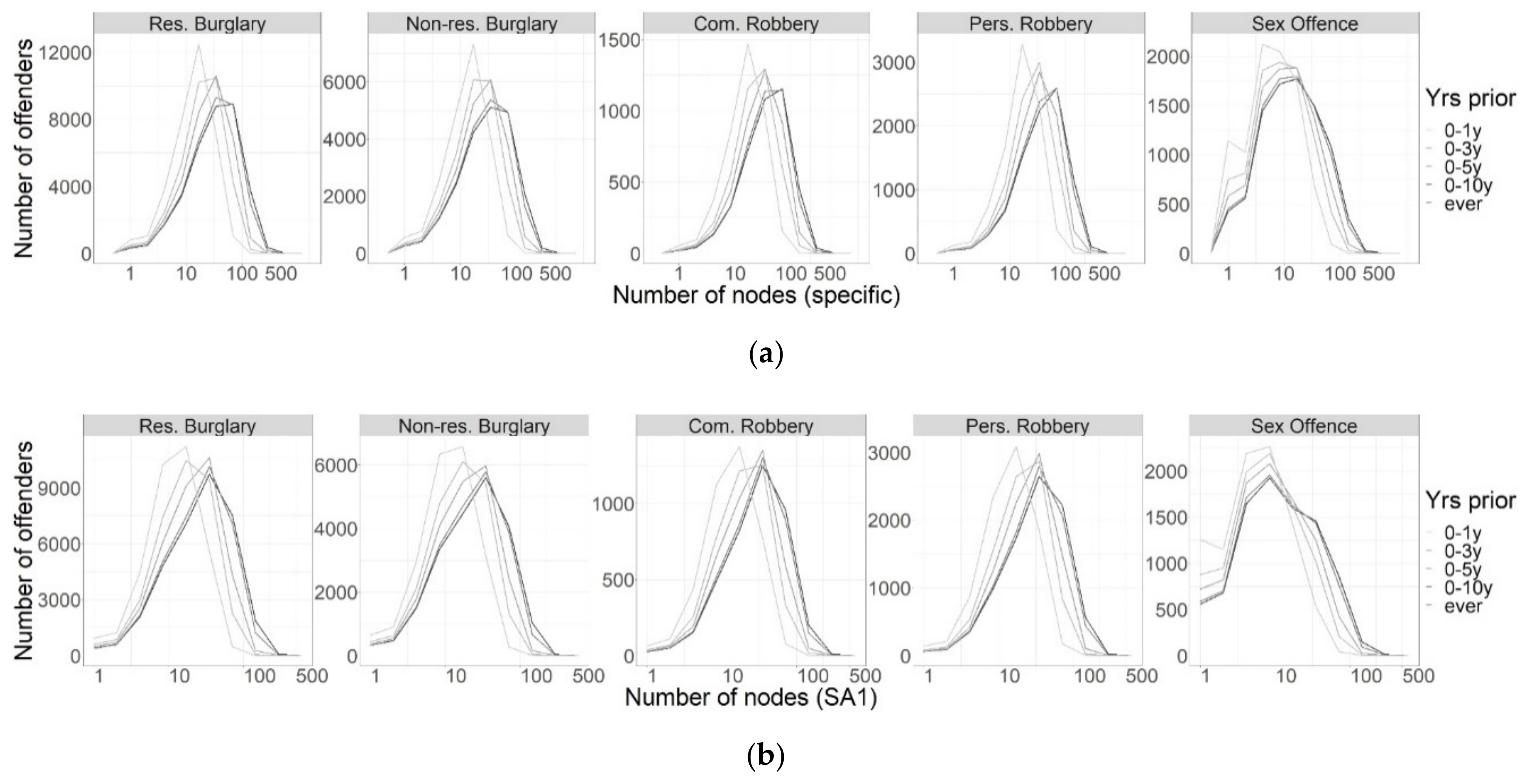
3.1. Number of Activity Nodes

Figure 2 presents the distributions of the number of activity nodes per offender, by offense type and pre-offense timeframe, for specific coordinates (top) and SA1s (bottom). The number of specific locations per offender ranged from 1 to 581 and the distributions are highly skewed: most offenders have a small number of nodes, and a small number of offenders have many nodes. The number of nodes increases with the length of the pre-offense period: as is to be expected since the measure is cumulative. The medians were comparable for burglary (from 14 for one year to 36 “ever”) and robbery (16 to 43) but smaller for sex offenses (6 to 13).

The number of SA1s per offender followed much the same distributions, except in the upper extremes. The median number of SA1s per offender ranged from 13/12 (0–1y) to 29/29 (“ever”) for residential/non-residential burglary, 14/15 to 32/24 for commercial/personal robbery and 5 to 11 for sex offenses. The maximum number of SA1s per offender was 481. As shown in Figure 1, distributions are very similar when comparing the top and bottom graphs, though the tails at the upper end of the distribution are truncated when specific locations are aggregated to SA1 resolution. This suggests a) that for most offenders, their few nodes are distributed among different SA1s and b) for the few offenders with many nodes, many of those nodes are clustered within SA1s.

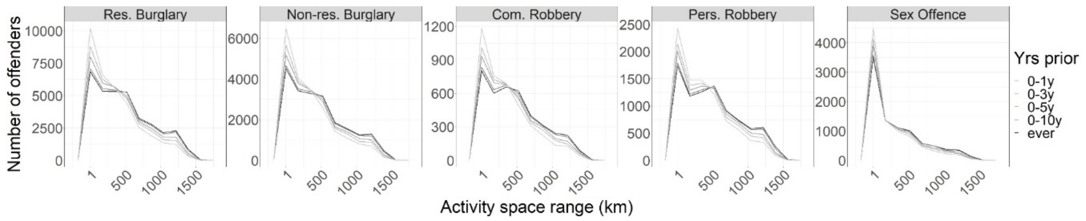
3.2. Activity Space Size

To put the number of SA1 nodes into a geographic context, 49.3% of offender SA1 nodes were located in the most populated urban TAs in NZ: Auckland, Wellington, Christchurch, and Hamilton. The numbers of SA1s per offender represent very small proportions of these urban areas, which contain between 1449 (Hamilton) and 13680 (Auckland) SA1s. For example, 13 SA1s represents 0.89% of Hamilton’s SA1s and 0.09% of Auckland’s; 29 represents 2.00% and 0.12% respectively; and the maximum of 421 (if they were all in the same city) represents 29.05%. and 3.08%. The activity spaces of offenders as recorded in police data, therefore, are typically constrained to a small portion of any given urban area in which they conduct their routine activities.

The distributions of activity space ranges, however, reveal that these activities are frequently distributed across multiple urban areas (while limited to small areas within each), as shown in Figure 3. The median distance range was 267 km/256 km for residential/non-residential burglary for 1 year (420 km/395 km ever), 268 km/319 km for commercial/personal robbery for 1 year (417/457 ever) and 78 km for sex offenses for 1 year (202 km ever). The maximum distance range was between 1400 and 1600 km for all offense types and activity node timeframes, representing nodes at opposite ends of the country (lengthwise). Interestingly, these maxima emerged early, appearing in the one-year pre-offense activity space timeframe. However, with increasing pre-offense time spans, there were increasing numbers of offenders whose activity spaces spanned multiple cities at greater distances apart.

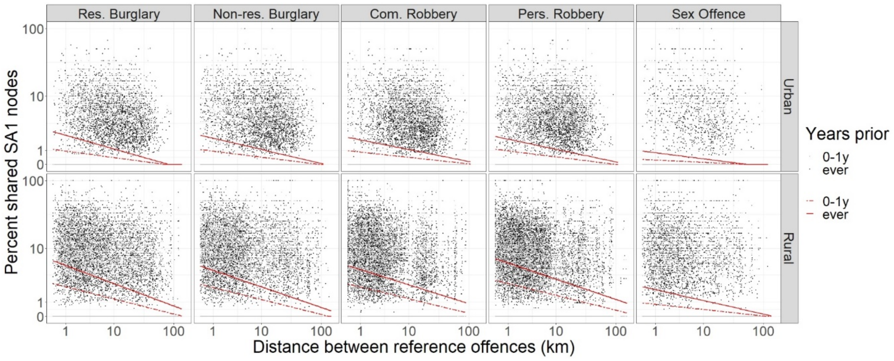
3.3. Shared Activity Space

Most offenders shared most or all of their activity nodes with at least one other offender (Figure 4, top). This is perhaps unsurprising given the volume and geographic spread of activity nodes, which would increase the likelihood of shared SA1s. Correspondingly, residential burglars, with the highest volumes of activity nodes, had larger proportions of SA1s shared with other residential burglars, while commercial robbers and sex offenders, with the lowest volumes of activity nodes, had smaller proportions of shared SA1s. Also as expected, the proportion of shared activity space increased as more activity nodes were included with increasing time prior to the reference offense (illustrated in Figure 4 by the darker lines extending higher on the y axis than the lighter lines, at upper limit of 100% on the x axis).

Even the proportion of activity space falling in the 25% most common SA1s was greater than 50% for most offenders (Figure 3, bottom). The medians were 68%/67% for one year to 68%/68% for residential/non-residential burglary, 58%/67% to 69%/70% for commercial/personal robbery and 52–56% for sex offenses. The upturns of the distributions at 0% and 100% shared reflect cases where offenders only have one activity node, meaning either all or no activity space is shared. Note also that the number of offenders sharing the 25% most common SA1s is relative to offense type. For example, the top 25% of SA1s for residential burglary offender nodes “ever” were shared by 55 or more offenders; the top 25% of SA1s for sex offender nodes “ever” were shared by 9 or more offenders.

Overall, these results point to a lack of distinctiveness in offender activity spaces recorded in police data, in that any given node is likely to be shared. The following analyses provide insight into whether the shared portions of individuals’ activity space are shared with the same or different offenders.

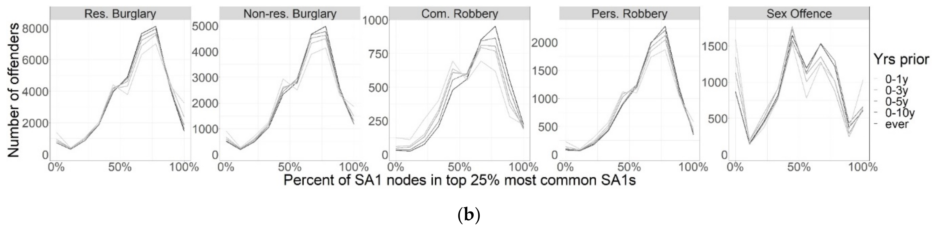
3.4. Homology and Differentiation

There were statistically significant but small correlations between the proximity of offenders’ reference offenses and the spatial similarity of their activity spaces. As shown by the fitted regression lines in red in Figure 5, broadly, the closer the reference offenses, the more shared activity space; the farther away the reference offenses, the less shared activity space. The correlations ranged from −0.07 for urban sex offenders’ 1-year pre-offense activity space to −0.24 for rural burglars’ “ever” (see Supplementary Material S5 for full results). The higher correlations for rural offenders on this measure are likely a product of the larger SA1s in rural areas, increasingly the likelihood of offenses and activity nodes falling into the same SA1.

Notably, the proportion of activity space shared between specific offender pairs is much smaller than that shared with offenders in general (see previous section), suggesting heterogeneity in offenders’ activity spaces. In Figure 5 about half of the offender pair points appear at 0% on the y axes. The median percentage shared activity space was 0% for all groups except rural residential burglars (2.1%), rural commercial robbers (3.0%) and rural personal robbers (4.5%). Almost no offender pairs shared 100% of their activity space.

As Figure 6 shows, to some extent, the closer any two offenders’ reference offenses, the closer together their nearest activity nodes; the farther away their offenses, the farther apart their nearest nodes. The correlations ranged from 0.14 for urban commercial robbers’ pre-offense activity space “ever”, to 0.29 for rural burglars’ 1-year pre-offense activity space (see Supplementary Material S5 for all results).

As shown in Figure 7, there was a general tendency that the closer any two offenders’ reference offenses, the closer their activity nodes on average; the farther away their offenses, the farther apart their nodes. The correlations ranged from 0.15 for rural commercial robbers’ pre-offense activity space “ever”, to 0.28 for urban burglars’ 1-year pre-offense activity space (see Supplementary Material S5 for all results).

Correlations were slightly weaker for the median nearest node distance than the minimum node distance for rural offenders. In contrast, correlations were slightly stronger for the median nearest node distance for urban burglary and robbery offenders. These small differences are potentially explained by the longer distances between nodes for rural offenders; urban offenders’ nodes would be closer together.

Burglars showed the strongest homology between offense proximity and activity space similarity, with very similar results for residential and non-residential burglars. Likewise, there were near identical results for commercial and personal robbers, both displaying less homology than burglars. Sex offenders showed the least homology as measured by percent shared activity space but more than robbers in terms of the distance between activity nodes.

Of pairs of offenders who offended in the same location, co-offenders shared more activity space, and had more proximal activity nodes than independent offenders. All tests of difference between co-offenders and other same location offenders were statistically significant, with small to moderate effect sizes (see Supplementary Material S6 for full results). On average, robbery and residential burglary co-offenders shared at least one exact location node (specific coordinates) in the “ever” timeframe, as indicated by median minimum node distances of 0. The minimum distance between nodes was under 200 m on average for burglary and robbery co-offenders, and under 500 m for independent burglars and robbers. Co-offending and independent sex offenders were less likely to share any nodes (specific coordinates or SA1s); their nearest nodes were also further apart on average (co-offenders: 50–540 m, independent: 280 m–1.86 km). Notably, even among co-offenders, the median distance from each of one co-offender’s nodes to the nearest of the other co-offender’s nodes was much longer, on average, than the minimum distance between their nodes.

Collectively these results suggest that offenders who offend in spatially similar locations tend to be spatially similar in parts of their activity space, though not necessarily in its entirety. Furthermore, these homology results are not solely attributable to co-offending. However, we also confirmed that co-offenders displayed greater activity space similarity than offenders who offended in the same location separately.

4. Discussion

We used routinely collected police data to provide insight into offenders’ activity spaces in terms of the number of activity nodes, their geographic range, and the extent to which they are shared between or differentiate offenders. We believe this to be the largest and most comprehensive study of offender activity space to date, considering the frequency and types of activity nodes included.

On the surface the one-year activity node distributions appear comparable to the results of Rossmo et al.’s [29] study of US parolees and Menting [28] and Bernasco’s [27] studies of young Dutch offenders, considering the different timeframes involved. Our medians were 13 to 15 for burglary/robbery and 5 for sex offenses, for nodes that were current during the year prior to the reference offense, compared with 4-7 nodes in the above studies over much shorter timeframes. However, our distributions were wider and appeared more skewed: a minority of offenders had no prior activity nodes on record; many offenders had few nodes; a few had very many. This result is likely a combination of both missingness and reality: we have more complete data for some individuals than for others, and some individuals genuinely have more activity nodes than others, as found in criminal cohorts in the 3 studies above and in the general population [51,56,59,60]. Future research could help establish the extent of (in)completeness by comparing police data at an individual level with alternative data sources such as surveys or GPS data as used in the studies above.

That the activity spaces frequently spanned multiple urban areas is consistent with the few NZ studies of the distances between offenders’ home addresses and their offenses, and of the mobility of New Zealanders in general. In NZ, the home-crime distances of sex offenders tend to be longer on average than overseas, with higher proportions of “commuter” offenders whose homes are outside the radius of their offenses [61,62,63,64]. Davidson’s [65] study of Christchurch burglars’ home-crime distances found more geographically constrained patterns but may not represent contemporary trends, given changes in societal travel patterns and mobility. In 21st Century New Zealand, people move frequently [66], family and friends can be widely dispersed across different towns and cities, and domestic travel by car or plane is common, despite the long distances involved [67,68,69,70,71,72]. The inclusion of prisons as activity nodes, sometimes recorded in the address data, would also have contributed to these distances because offenders may be transferred to prisons a long way from their community; they may also not return to the same community on release [73] (Prison addresses were not always readily identifiable in the data, precluding a comprehensive investigation into the extent to which they accounted for wide activity space ranges.). It is no surprise, therefore, that NZ offenders’ activity spaces spanned much longer distances than those of the offenders studied by Rossmo et al. [29], Menting [28] and Bernasco [27], given these studies were more geographically and temporally constrained, and involved cohorts with likely more limited mobility (offenders on GPS monitoring and young people). However, the extent to which our results are unique to New Zealand or indicate that offender populations have wider activity ranges than captured by studies with smaller study areas warrants further investigation. We encourage future studies of offender activity space in other countries to widen their spatial scope.

The analyses of the number and geographic range of activity nodes reveal potential and problems for the use of this data in research and practice. In terms of volume, the data are promising: there were a variety of activity nodes beyond home addresses available for the burglary, robbery and—to a lesser extent—sex offenders included in this study. There was also considerable information gain when extending the timeframe to less recent activity nodes (burglary median 29 nodes, robbery 34, sex offenses 11), though it remains for future research to explore whether this additional information yields any signal: we do not yet know whether these “older” activity nodes bear on the locations of future offenses. In contrast, the distributions were very similar regardless of the unit of analysis, which may partly reflect the small size of SA1s in the urban areas in which activity nodes were concentrated. Research and analysis may therefore benefit from the use of aggregate spatial units of SA1 size without much loss of information, at least in urban areas.

The geographic span of the offenders’ activity spaces indicates a potential limitation of this data. Given that offenders’ activity nodes were often widely dispersed, a high proportion of these nodes are likely to have little bearing on their choice of crime locations at a micro-geographic or neighborhood level. There may even be no activity nodes known to police in proximity to offenders’ latest offense locations. In crime location choice research, if the data do not include—with sufficient frequency—the more proximal activity nodes likely to have influenced a given crime location choice, models may fail to identify relationships between activity nodes and crime locations. In crime investigations, there is potential to miss possible suspects by narrowly focusing on those with local nodes in police data, highlighting the importance of supplementing police information with other sources of information on suspects’ activity nodes, be it through data sharing agreements with other agencies or on an individual basis for named suspects in a given investigation.

Any given activity node (SA1) was likely to be shared with other offenders who had committed the same reference offense, though these nodes were not necessarily “active” at the same time. This result is consistent with Hart and colleagues’ [60] finding that 80% of the paths between young Australians’ activity nodes were shared. The most frequently shared nodes reflected places expected to have high numbers of offenders residing or visiting (prisons, police stations, court houses) or high numbers of people in general (consistent with the findings of Menting et al. [20]). The latter would generate more activity node records in police data through higher levels of crime opportunity and higher odds of encountering police during proactive patrols.

Comparing any two offenders, however, showed much less overlap between their particular activity spaces, signaling considerable individual differences in offenders’ routine activity patterns as captured in this data. The homology and differentiation results suggest that those routine activity spaces were—marginally—more likely to converge the closer together offenders’ latest offenses were. Our results thus provide evidence of a small degree of spatial homology and differentiation, and some insights into its causes.

For example, reference offense co-offenders had greater activity space similarity than offenders who offended in the same location but independently. One potential explanation for this finding is that it reflects co-offenders who have also committed other crimes together in the past, and who thus share prior crime nodes. Other potential explanations reflect possible familial or social connections between co-offenders. On occasion, co-offenders may be family members [74,75], who may therefore share home addresses, family home address, or school nodes. However, more frequently, co-offenders are connected socially [76,77]. Human mobility studies have shown that people more closely connected in a social network have more similar activity spaces than those who are not socially connected [78,79,80,81]. Co-offenders’ social ties could be a product of living in close proximity or attending the same school, and both a cause and effect of sharing “hangout” nodes [77,82,83]. In NZ, as elsewhere, co-offending can occur as a part of membership of gangs, from the fluid, loosely connected structures of youth gangs, to more hierarchical organized crime groups [84,85,86,87,88]. Many youth gangs align themselves to particular neighborhoods reflective of the shared activity space of their members, and more formalized gangs are arranged into local “chapters” [84,85,86]. Consistent with Lammers’ study [35], however, co-offenders did not share most of their activity nodes.

However, since co-offenders only made up a small proportion of offender pairs used for the homology correlations (and excluding them made no difference to the results), other mechanisms must be at play. For example, those who share activity space are likely to become aware of the same criminal opportunities; those with different activity spaces are exposed to different opportunities. Social networks also play a role: previous co-offenders (who share prior crime nodes) share information with each other about crime opportunities that influences where they offend in the future not only together but separately [89,90].

Robbery offenders displayed less homology than burglars. This could be expected since robbery tends to concentrate in commercial areas with high numbers of potential targets [13,91,92], which would attract potential offenders with disparate residential nodes [2,34]. That homology was still present may reflect the range of nodes in the data: offenders committing robberies in the same commercial area may also have committed prior offenses or have had prior interactions with police in the vicinity.

Those committing sex offenses appear to be a more spatially heterogenous group, also displaying less spatial overlap or proximity in their activity spaces. This might be an effect of there being fewer nodes in the dataset for these offenders, which would mean less chance of finding overlapping or proximal nodes. It might also be an effect of the heterogenous nature of these offenses. The sex offenses included a wide range of behaviors, from indecent exposure to rape, and included offenses against children and adults. They could have occurred at the offender’s home, the victim’s home, or elsewhere [93,94,95,96,97]. Sex offenders’ strategies for identifying, approaching, and attacking victims vary widely from extended grooming to opportunistic “blitz” attacks [98,99,100,101,102]. Offenders might identify their victims through social networks (online or offline) or search for victims in target rich environments such as near schools or night-time economy districts [94,96,97,102,103,104]. All these factors would lead to variation in the relationship between offenders’ activity spaces and their crime locations. Furthermore, social connection and sharing of information between sex offenders, such as about the locations of criminal opportunities, appears to be less common than with property crime [97], which would reduce network driven homology effects. Future research might seek to isolate spatial homology effects for different subtypes of sex offenders.

Several limitations of the data are also worth considering in interpreting our results. First, the data only identifies co-offenders where there was sufficient evidence to proceed against each offender. In some cases, multiple offenders may have been involved in a crime but not recorded as offenders due to a lack of evidence. Furthermore, offender pairs were only identifiable as co-offenders if the offense was both offenders’ reference (i.e., latest) offense. Offender pairs would not be identified as co-offenders if one had committed a subsequent offense. To the extent that any co-offenders were thus treated as having offended independently, the differences between co-offenders and independent offenders will have been under-estimated.

Second, the data were not systematically recorded; they were only on file where collected for operational purposes. As noted, some offenders had more complete records, representing more of their routine activity space. Our conclusions are therefore limited to offenders’ activity spaces to the extent identifiable by routinely collected police data.

An additional caveat is that not all activity space is equal with respect to crime location choice. Activity nodes that are more recent, more frequently visited, and have been in activity space for a longer time have stronger associations with crime locations [27,28,105], as do activity nodes that provide the most relevant knowledge of criminal opportunity: prior crimes of the same nature [26,106]. We could therefore expect greater spatial similarity in those parts of offenders’ activity spaces that have had the greatest influence in producing similarity of their crime locations. Indeed, our results suggest that offenders who offend in spatially similar locations are spatially similar in parts of their activity space. Further research would be needed to determine, with the present dataset, which activity nodes are most predictive of crime locations, and whether homology effects are larger when activity space is isolated to, or weighted by, these most influential activity nodes.

5. Conclusions

Our exploration of police data on a wider range of activity nodes than included in previous studies suggests that geographic crime analysis and research could benefit from the use of such datasets, though with some caution. Our findings in relation to the distances within and between offenders’ activity nodes—and the implications we have highlighted for research and practice—are likely to generalize to other countries with similar levels of internal mobility and dispersed populations (at both micro and macro geographic scales). In addition, our findings in relation to the sparsity, and heterogeneity, of sex offenders’ activity nodes in this data are also likely to apply to equivalent datasets in other jurisdictions. However, despite these limitations, the data provided new direct evidence of the applicability of the homology and differentiation “profiling assumptions” in the geographic profiling context of offenders’ offense locations and activity spaces. We encourage further research, with data from police and alternative sources, into the specific elements of activity space that display greater homology and differentiation with respect to offenders’ crime locations, and which could further support geographic profiling by enabling specific nodes of potential suspects to receive more weight in prioritization decisions.

References

1. Brantingham, P.L.; Brantingham, P.J. Notes on the geometry of crime. In Environmental Criminology; Waveland Press: Prospect Heights, IL, USA, 1991; pp. 27–54. ISBN 978-0-8039-1678-4. [Google Scholar]
2. Brantingham, P.L.; Brantingham, P.J. Environment, routine, and situation: Toward a pattern theory of crime. In Routine Activity and Rational Choice-Advances in Criminological Theory; Clarke, R.V., Felson, M., Eds.; Transaction Publishers: Piscataway, NJ, USA, 1993; pp. 259–294. ISBN 978-1-56000-087-7. [Google Scholar]
3. Ruiter, S. Crime location choice. In The Oxford Handbook of Offender Decision Making; Bernasco, W., Van Gelder, J.-L., Elffers, H., Eds.; Oxford University Press: Oxford, UK, 2017; pp. 398–420. [Google Scholar]
4. Curtis-Ham, S.; Bernasco, W.; Medvedev, O.N.; Polaschek, D. A Framework for Estimating Crime Location Choice Based on Awareness Space. Crime Sci. 2020, 9, 1–14. [Google Scholar] [CrossRef]
5. Chesher, C. Digitising the Beat: Police Databases and Incorporeal Transformations. Convergence 1997, 3, 72–81. [Google Scholar] [CrossRef]
6. Garicano, L.; Heaton, P. Information Technology, Organization, and Productivity in the Public Sector: Evidence from Police Departments. J. Labor Econ. 2010, 28, 167–201. [Google Scholar] [CrossRef] [Green Version]
7. Home Office National Law Enforcement Data Programme. Law Enforcement Data Service (LEDS)–Privacy Impact Assessment Report; Home Office: London, UK, 2018.
8. Schellenberg, K. Police Information Systems, Information Practices and Individual Privacy. Can. Public Policy 1997, 23, 23–39. [Google Scholar] [CrossRef]
9. Long, D.; Liu, L.; Feng, J.; Zhou, S. Assessing the Influence of Prior on Subsequent Street Robbery Location Choices: A Case Study in ZG City, China. Sustainability 2018, 10, 1818. [Google Scholar] [CrossRef] [Green Version]
10. Canter, D. Geographical profiling of criminals. In Principles of Geographical Offender Profiling; Canter, D., Youngs, D., Eds.; Ashgate: Aldershot, UK, 2008; pp. 259–270. ISBN 978-0-7546-2547-6. [Google Scholar]
11. Rossmo, D.K. Geographic Profiling; CRC Press: Boca Raton, FL, USA, 2000; ISBN 0-8493-8129-0. [Google Scholar]
12. Cohen, L.E.; Felson, M. Social Change and Crime Rate Trends: A Routine Activity Approach. Am. Sociol. Rev. 1979, 44, 588–608. [Google Scholar] [CrossRef]
13. Weisburd, D.; Eck, J.E.; Braga, A.A.; Telep, C.W.; Cave, B.; Bowers, K.; Bruinsma, G.J.N.; Gill, C.; Groff, E.R.; Hibdon, J.; et al. Place Matters: Criminology for the Twenty-First Century; Cambridge University Press: Cambridge, UK, 2016. [Google Scholar]
14. Weisburd, D. The Law of Crime Concentration and the Criminology of Place. Criminology 2015, 53, 133–157. [Google Scholar] [CrossRef]
15. Townsley, M. Offender mobility. In Environmental Criminology and Crime Analysis; Wortley, R., Townsley, M., Eds.; Routledge: London, UK, 2016; pp. 142–161. ISBN 978-1-317-48710-4. [Google Scholar]
16. Canter, D.; Hodge, S. Criminals’ mental maps. In Atlas of Crime: Mapping the Criminal Landscape; Turnbull, L., Hendrix, E., Dent, B., Eds.; Oryx Press: Phoenix, AZ, USA, 2000; pp. 186–191. [Google Scholar]
17. Davies, A.; Dale, A. Locating the Stranger Rapist. Med. Sci. Law 1996, 36, 146–156. [Google Scholar] [CrossRef]
18. Pettiway, L.E. Copping Crack: The Travel Behavior of Crack Users. Justice Q. 1995, 12, 499–524. [Google Scholar] [CrossRef]
19. Rengert, G.; Wasilchick, J. Suburban Burglary: A Time and a Place for Everything; C.C. Thomas: Springfield, IL, USA, 1985; ISBN 978-0-398-05142-6. [Google Scholar]
20. Summers, L.; Johnson, S.D.; Rengert, G. The use of maps in offender interviewing. In Offenders on Offending: Learning about Crime from Criminals; Bernasco, W., Ed.; Willan: Collumpton, Devon, UK, 2010; pp. 246–272. [Google Scholar]
21. van Daele, S. Itinerant crime groups: Mobility attributed to anchor points? In Contemporary Issues in the Empirical Study of Crime; Governance of Security Research Paper Series; Pauwels, L., Ponsaers, P., Vande Walle, G., Vander Beken, T., Vander Laenen, F., Vermeulen, G., Cools, M., De Kimpe, S., De Ruyver, B., Easton, M., Eds.; Maklu: Antwerp, Belgium, 2009; Volume 1, pp. 211–225. [Google Scholar]
22. Wiles, P.; Costello, A. The “road to nowhere”: The evidence for travelling criminals. In Principles of Geographical Offender Profiling; Canter, D., Youngs, D., Eds.; Ashgate: Aldershot, UK, 2008; pp. 165–175. [Google Scholar]
23. Frith, M.J. Modelling Taste Heterogeneity Regarding Offence Location Choices. J. Choice Model. 2019, 33, 100187. [Google Scholar] [CrossRef]
24. Menting, B. Awareness × Opportunity: Testing Interactions between Activity Nodes and Criminal Opportunity in Predicting Crime Location Choice. Br. J. Criminol. 2018, 58, 1171–1192. [Google Scholar] [CrossRef]
25. Menting, B.; Lammers, M.; Ruiter, S.; Bernasco, W. Family Matters: Effects of Family Members’ Residential Areas on Crime Location Choice. Criminology 2016, 54, 413–433. [Google Scholar] [CrossRef]
26. Van Sleeuwen, S.E.M.; Ruiter, S.; Menting, B. A Time for a Crime: Temporal Aspects of Repeat Offenders’ Crime Location Choices. J. Res. Crime Delinq. 2018, 55, 538–568. [Google Scholar] [CrossRef]
27. Bernasco, W. Adolescent Offenders’ Current Whereabouts Predict Locations of Their Future Crimes. PLoS ONE 2019, 14, e0210733. [Google Scholar] [CrossRef]
28. Menting, B.; Lammers, M.; Ruiter, S.; Bernasco, W. The Influence of Activity Space and Visiting Frequency on Crime Location Choice: Findings from an Online Self-Report Survey. Br. J. Criminol. 2020, 60, 303–322. [Google Scholar] [CrossRef]
29. Rossmo, D.K.; Lu, Y.; Fang, T.B. Spatial-temporal crime paths. In Patterns, Prevention, and Geometry of Crime; Andresen, M.A., Kinney, J.B., Eds.; Routledge: London, UK, 2012; pp. 3–15. [Google Scholar]
30. Rossmo, D.K.; Rombouts, S. Geographic profiling. In Environmental Criminology and Crime Analysis; Wortley, R., Mazerolle, L., Eds.; Willan: Collumpton, Devon, UK, 2008; pp. 136–149. [Google Scholar]
31. Canter, D. Offender Profiling and Criminal Differentiation. Leg. Criminol. Psychol. 2000, 5, 23–46. [Google Scholar] [CrossRef] [Green Version]
32. Doan, B.; Snook, B. A Failure to Find Empirical Support for the Homology Assumption in Criminal Profiling. J. Police Crim. Psychol. 2008, 23, 61–70. [Google Scholar] [CrossRef]
33. Woodhams, J.; Toye, K. An Empirical Test of the Assumptions of Case Linkage and Offender Profiling with Serial Business Robberies. Psychol. Public Policy Law 2007, 13, 59–85. [Google Scholar] [CrossRef]
34. Costanzo, C.; Halperin, W.; Gale, N. Criminal mobility and the directional component in journeys to crime. In Metropolitan Crime Patterns; Figlio, R., Hakim, S., Rengert, G., Eds.; Criminal Justice Press: Monsey, NY, USA, 1986; pp. 73–96. [Google Scholar]
35. Lammers, M. Co-Offenders’ Crime Location Choice: Do Co-Offending Groups Commit Crimes in Their Shared Awareness Space? Br. J. Criminol. 2018, 58, 1193–1211. [Google Scholar] [CrossRef]
36. Tayebi, M.A.; Frank, R.; Glässer, U. Understanding the Link between Social and Spatial Distance in the Crime World. In Proceedings of the 20th International Conference on Intelligent User Interfaces, Redondo Beach, CA, USA, 6 November 2012. [Google Scholar]
37. Malm, A.; Kinney, J.B.; Pollard, N. Social Network and Distance Correlates of Criminal Associates Involved in Illicit Drug Production. Secur. J. 2008, 21, 77–94. [Google Scholar] [CrossRef]
38. Bernasco, W. Them Again?: Same-Offender Involvement in Repeat and near Repeat Burglaries. Eur. J. Criminol. 2008, 5, 411–431. [Google Scholar] [CrossRef] [Green Version]
39. Haginoya, S.; Hanayama, A.; Koike, T. Linkage Analysis Using Geographical Proximity: A Test of the Efficacy of Distance Measures. J. Criminol. Res. Policy Pr. 2020. [Google Scholar] [CrossRef]
40. Johnson, S.D.; Summers, L.; Pease, K. Offender as Forager? A Direct Test of the Boost Account of Victimization. J. Quant. Criminol. 2009, 25, 181–200. [Google Scholar] [CrossRef]
41. Tonkin, M.; Woodhams, J.; Bull, R.; Bond, J.W.; Palmer, E.J. Linking Different Types of Crime Using Geographical and Temporal Proximity. Crim. Justice Behav. 2011, 38, 1069–1088. [Google Scholar] [CrossRef]
42. Tonkin, M.; Santtila, P.; Bull, R. The Linking of Burglary Crimes Using Offender Behaviour: Testing Research Cross-Nationally and Exploring Methodology. Leg. Criminol. Psychol. 2012, 17, 276–293. [Google Scholar] [CrossRef] [Green Version]
43. De Montjoye, Y.-A.; Hidalgo, C.; Verleysen, M.; Blondel, V. Unique in the Crowd: The Privacy Bounds of Human Mobility. Sci. Rep. 2013, 3, 1376. [Google Scholar] [CrossRef] [Green Version]
44. Yeoman, A.; Cook, L.W. The Kiwi Nest: 60 Years of Change in New Zealand Families; Families Commission: Wellington, New Zealand, 2008.
45. R Core Team. R: A Language and Environment for Statistical Computing.; R Foundation for Statistical Computing: Vienna, Austria, 2013. [Google Scholar]
46. Andresen, M.A.; Malleson, N.; Steenbeek, W.; Townsley, M.; Vandeviver, C. Minimum Geocoding Match Rates: An International Study of the Impact of Data and Areal Unit Sizes. Int. J. Geogr. Inf. Sci. 2020, 34, 1306–1322. [Google Scholar] [CrossRef]
47. Briz-Redón, Á.; Martinez-Ruiz, F.; Montes, F. Re-Estimating a Minimum Acceptable Geocoding Hit Rate for Conducting a Spatial Analysis. Int. J. Geogr. Inf. Sci. 2019, 34, 1283–1305. [Google Scholar] [CrossRef]
48. Bernasco, W. Modeling Micro-Level Crime Location Choice: Application of the Discrete Choice Framework to Crime at Places. J. Quant. Criminol. 2010, 26, 113–138. [Google Scholar] [CrossRef]
49. Hanson, S.; Huff, O.J. Systematic Variability in Repetitious Travel. Transportation 1988, 15, 111–135. [Google Scholar] [CrossRef]
50. Pappalardo, L. The Origin of Heterogeneity in Human Mobility Ranges. In Proceedings of the CEUR Workshop Proceedings CEUR-WS, Bordeaux, France, 15 March 2016. [Google Scholar]
51. Pappalardo, L.; Simini, F.; Rinzivillo, S.; Pedreschi, D.; Giannotti, F.; Barabási, A.-L. Returners and Explorers Dichotomy in Human Mobility. Nat. Commun. 2015, 6, 8166–8173. [Google Scholar] [CrossRef] [PubMed] [Green Version]
52. Schönfelder, S.; Axhausen, K.W. Measuring the Size and Structure of Human Activity Spaces: The Longitudinal Perspective; ETH: Zurich, Switzerland, 2002. [Google Scholar]
53. Pebesma, E. Simple Features for R: Standardized Support for Spatial Vector Data. R J. 2018, 10, 439. [Google Scholar] [CrossRef] [Green Version]
54. Patterson, Z.; Farber, S. Potential Path Areas and Activity Spaces in Application: A Review. Transp. Rev. 2015, 35, 679–700. [Google Scholar] [CrossRef]
55. Mokros, A.; Alison, L.J. Is Offender Profiling Possible? Testing the Predicted Homology of Crime Scene Actions and Background Characteristics in a Sample of Rapists. Leg. Criminol. Psychol. 2002, 7, 25–43. [Google Scholar] [CrossRef]
56. Alessandretti, L.; Sapiezynski, P.; Sekara, V.; Lehmann, S.; Baronchelli, A. Evidence for a Conserved Quantity in Human Mobility. Nat. Hum. Behav. 2018, 2, 485–491. [Google Scholar] [CrossRef]
57. Canter, D.; Shalev, K. Putting crime in its place: A psychological process in crime site selection. In Principles of Geographical Offender Profiling; Canter, D., Youngs, D., Eds.; Ashgate: Aldershot, UK, 2008; pp. 259–270. ISBN 978-0-7546-2547-6. [Google Scholar]
58. Marchment, Z.; Bouhana, N.; Gill, P. Lone Actor Terrorists: A Residence-to-Crime Approach. Terror. Political Violence 2018, 1–26. [Google Scholar] [CrossRef]
59. González, M.C.; Hidalgo, C.A.; Barabási, A.-L. Understanding Individual Human Mobility Patterns. Nature 2008, 453, 779–782. [Google Scholar] [CrossRef]
60. Hart, T.C.; Birks, D.; Townsley, M.; Ruiter, S.; Bernasco, W. Activity nodes, activity spaces, and awareness spaces: Measuring geometry of crime’s constructs with smartphone data. In Space, Time, and Crime; Hart, T.C., Lersch, K.M., Chataway, M., Eds.; Carolina Academic Press: Durham, NC, USA, 2020; pp. 156–176. ISBN 978-1-5310-1540-4. [Google Scholar]
61. Hammond, L. Geographical Profiling in a Novel Context: Prioritising the Search for New Zealand Sex Offenders. Psychol. Crime Law 2014, 20, 358–371. [Google Scholar] [CrossRef] [Green Version]
62. Lundrigan, S.; Czarnomski, S.; Wilson, M. Spatial and Environmental Consistency in Serial Sexual Assault. J. Investig. Psych. Offender Profil. 2010, 7, 15–30. [Google Scholar] [CrossRef] [Green Version]
63. Lundrigan, S.; Czarnomski, S. Spatial Characteristics of Serial Sexual Assault in New Zealand. Aust. N. Z. J. Criminol. 2006, 39, 218–231. [Google Scholar] [CrossRef]
64. Scott, D. The Travelling Distances of Stranger Intruder Sex Offenders; New Zealand Police: Wellington, New Zealand, 2012.
65. Davidson, R.N. Patterns of Residential Burglary in Christchurch. N. Z. Geogr. 1980, 36, 73–78. [Google Scholar] [CrossRef]
66. Superu. Residential Movement within New Zealand: Quantifying and Characterising the Transient Population; Social Policy Evaluation and Research Unit: Wellington, New Zealand, 2018.
67. Ministry of Transport. 25 Years of New Zealand Travel: New Zealand Household Travel 1989–2014; Ministry of Transport: Wellington, New Zealand, 2015.
68. Ministry of Transport. New Zealand Household Travel Survey 2015–2017; Ministry of Transport: Wellington, New Zealand, 2017.
69. Ministry of Transport. Transport Outlook Current State 2016: A Summary of New Zealand’s Transport System; Ministry of Transport: Wellington, New Zealand, 2017.
70. Ministry of Transport. Inter-Regional Ground Travel by Residents. Available online: https://www.transport.govt.nz/mot-resources/research-papers/inter-regional-ground-travel-data-from-qrious/ (accessed on 1 April 2020).
71. Vuletich, S.; Becken, S. The Tourism Flows Model: Summary Document; Ministry of Tourism: Wellington, New Zealand, 2007.
72. Witten, K.; Huakau, J.; Mavoa, S. Social and Recreational Travel: The Destinations, Travel Modes and CO2 Emissions of New Zealand Households. Soc. Policy J. N. Z. 2011, 37, 172–184. [Google Scholar]
73. Robson, S.; Yesberg, J.A.; Wilson, M.S.; Polaschek, D.L.L. A Fresh Start or the Devil You Know? Examining Relationships between Release Location Choices, Community Experiences, and Recidivism for High-Risk Parolees. Int. J. Offender Ther. Comp. Criminol. 2019, 64, 35–653. [Google Scholar] [CrossRef] [PubMed]
74. Goldsmith, A.; Halsey, M. Cousins in Crime: Mobility, Place and Belonging in Indigenous Youth Co-Offending. Br. J. Criminol. 2013, 53, 1157–1177. [Google Scholar] [CrossRef]
75. Reiss, A.J., Jr.; Farrington, D.P. Advancing Knowledge about Co-Offending: Results from a Prospective Longitudinal Survey of London Males. J. Crim. Law Criminol. 1991, 82, 360–395. [Google Scholar] [CrossRef] [Green Version]
76. Mcgloin, J.M.; Povitsky Stickle, W. Influence or Convenience? Disentangling Peer Influence and Co-Offending for Chronic Offenders. J. Res. Crime Delinq. 2011, 48, 419–447. [Google Scholar] [CrossRef] [Green Version]
77. Weerman, F. Co-Offending as Social Exchange: Explaining Characteristics of Co-Offending. Br. J. Criminol. 2003, 43, 398–416. [Google Scholar] [CrossRef]
78. Liu, Z.; Qiao, Y.; Tao, S.; Lin, W.; Yang, J. Analyzing Human Mobility and Social Relationships from Cellular Network Data. In Proceedings of the 13th International Conference on Network and Service Management (CNSM), Tokyo, Japan, 26–30 November 2017; pp. 1–6. [Google Scholar]
79. Toole, J.L.; Herrera-Yaqüe, C.; Schneider, C.M.; González, M.C. Coupling Human Mobility and Social Ties. J. R. Soc. Interface 2015, 12, 20141128. [Google Scholar] [CrossRef] [Green Version]
80. Wang, D.; Pedreschi, D.; Song, C.; Giannotti, F.; Barabasi, A.-L. Human Mobility, Social Ties, and Link Prediction. In Proceedings of the 17th ACM SIGKDD International Conference on Knowledge Discovery and Data Mining, San Diego, CA, USA, 21–24 August 2011; pp. 1100–1108. [Google Scholar]
81. Xu, Y.; Belyi, A.; Bojic, I.; Ratti, C. How Friends Share Urban Space: An Exploratory Spatiotemporal Analysis Using Mobile Phone Data. Trans. GIS 2017, 21, 468–487. [Google Scholar] [CrossRef]
82. Felson, M. The process of co-offending. In Theory and Practice in Situational Crime Prevention; Smith, M.J., Cornish, D.B., Eds.; Criminal Justice Press: Monsey, NY, USA, 2003; pp. 149–167. [Google Scholar]
83. Schaefer, D.R. Youth Co-Offending Networks: An Investigation of Social and Spatial Effects. Soc. Netw. 2012, 34, 141–149. [Google Scholar] [CrossRef]
84. Centre for Social Research and Evaluation. From Wannabes to Youth Offenders: Youth Gangs in Counties Manukau; Ministry of Social Development: Wellington, New Zealand, 2008.
85. Eggleston, E.J. New Zealand Youth Gangs: Key Findings and Recommendations from an Urban Ethnography. Soc. Policy J. N. Z. 2000, 14. [Google Scholar]
86. Gilbert, J. Patched: The History of Gangs in New Zealand; Auckland University Press: Auckland, New Zealand, 2013; ISBN 978-1-86940-729-2. [Google Scholar]
87. New Zealand Parliament. Youth Gangs in New Zealand; New Zealand Parliamentary Service: Wellington, New Zealand, 2019.
88. Office of the Minister of Police. Whole-of-Government Action Plan to Reduce the Harms Caused by New Zealand Adult Gangs and Transnational Crime Groups; New Zealand Cabinet: Wellington, New Zealand, 2014.
89. McAndrew, D. The structural analysis of criminal networks. In The Social Psychology of Crime: Groups, Teams, and Networks; Canter, D., Alison, L., Eds.; Ashgate: Aldershot, UK, 2000; pp. 53–94. ISBN 978-1-84014-435-2. [Google Scholar]
90. Lantz, B.; Ruback, R.B. A Networked Boost: Burglary Co-Offending and Repeat Victimization Using a Network Approach. Crime Delinq. 2017, 63, 1066–1090. [Google Scholar] [CrossRef]
91. Browning, C.R.; Byron, R.A.; Calder, C.A.; Krivo, L.J.; Kwan, M.-P.; Lee, J.-Y.; Peterson, R.D. Commercial Density, Residential Concentration, and Crime: Land Use Patterns and Violence in Neighborhood Context. J. Res. Crime Delinq. 2010, 47, 329–357. [Google Scholar] [CrossRef]
92. Tillyer, M.S.; Walter, R.J. Busy Businesses and Busy Contexts: The Distribution and Sources of Crime at Commercial Properties. J. Res. Crime Delinq. 2019, 56, 816–850. [Google Scholar] [CrossRef]
93. Chopin, J.; Caneppele, S. The Mobility Crime Triangle for Sexual Offenders and the Role of Individual and Environmental Factors. Sex Abus. J. Res. Treat. 2018, 31, 812–836. [Google Scholar] [CrossRef]
94. Chopin, J.; Caneppele, S. Geocoding Child Sexual Abuse: An Explorative Analysis on Journey to Crime and to Victimization from French Police Data. Child Abus. Negl. 2019, 91, 116–130. [Google Scholar] [CrossRef]
95. Leclerc, B.; Wortley, R.; Smallbone, S. Investigating Mobility Patterns for Repetitive Sexual Contact in Adult Child Sex Offending. J. Crim. Justice 2010, 38, 648–656. [Google Scholar] [CrossRef] [Green Version]
96. Leclerc, B.; Felson, M. Routine Activities Preceding Adolescent Sexual Abuse of Younger Children. Sexual Abus. J. Res. Treat. 2016, 28, 116–131. [Google Scholar] [CrossRef]
97. Smallbone, S.W.; Wortley, R.K. Child Sexual Abuse in Queensland: Offender Characteristics & Modus Operandi; Queensland Crime Commission: Fortitude Valley, QLD, Australia, 2000.
98. Balemba, S.; Beauregard, E. Where and When? Examining Spatiotemporal Aspects of Sexual Assault Events. J. Sexual Aggress. 2013, 19, 171–190. [Google Scholar] [CrossRef]
99. Beauregard, E.; Rebocho, M.F.; Rossmo, D.K. Target Selection Patterns in Rape. J. Investig. Psych. Offender Profil. 2010, 7, 137–152. [Google Scholar] [CrossRef]
100. Beauregard, E.; Busina, I. Journey “during” Crime: Predicting Criminal Mobility Patterns in Sexual Assaults. J. Interpers. Violence 2013, 28, 2052–2067. [Google Scholar] [CrossRef] [PubMed]
101. Deslauriers-Varin, N.; Beauregard, E. Investigating Offending Consistency of Geographic and Environmental Factors among Serial Sex Offenders: A Comparison of Multiple Analytical Strategies. Crim. Justice Behav. 2013, 40, 156–179. [Google Scholar] [CrossRef]
102. Mogavero, M.C.; Hsu, K.-H. Sex Offender Mobility: An Application of Crime Pattern Theory among Child Sex Offenders. Sex. Abus. J. Res. Treat. 2017, 30, 908–931. [Google Scholar] [CrossRef] [PubMed]
103. Aslan, D. Critically Evaluating Typologies of Internet Sex Offenders: A Psychological Perspective. J. Forensic Psychol. Pr. 2011, 11, 406–431. [Google Scholar] [CrossRef]
104. Beauregard, E.; Rossmo, D.K.; Proulx, J. A Descriptive Model of the Hunting Process of Serial Sex Offenders: A Rational Choice Perspective. J. Fam. Violence 2007, 22, 449–463. [Google Scholar] [CrossRef]
105. Bernasco, W. A Sentimental Journey to Crime: Effects of Residential History on Crime Location Choice. Criminology 2010, 48, 389–416. [Google Scholar] [CrossRef]
106. Lammers, M.; Menting, B.; Ruiter, S.; Bernasco, W. Biting Once, Twice: The Influence of Prior on Subsequent Crime Location Choice. Criminology 2015, 53, 309–329. [Google Scholar] [CrossRef]
Figure 1. Illustration of activity space similarity measures for three pairs of offenders: (A) with close reference offenses and high activity space similarity on all three measures, (B) with close reference offenses and some activity space similarity, depending on measure, and (C) with distant reference offenses and less activity space similarity.
Ijgi 10 00047 g001
Figure 2. Distribution of activity nodes per offender by reference offense type and timeframe preceding the reference offense based on specific coordinates (a) and SA1 census units (b).
Ijgi 10 00047 g002
Figure 3. Distribution of activity space range per offender by reference offense type and timeframe preceding the reference offense.
Ijgi 10 00047 g003
Figure 4. Distribution of proportion of activity space shared with any other offenders (a) and in the top 25% most commonly shared SA1s (b), by reference offense type and timeframe preceding the reference offense.
Ijgi 10 00047 g004aIjgi 10 00047 g004b
Figure 5. Proportion of activity space shared between pairs of offenders by distance between their reference offenses.
Ijgi 10 00047 g005
Figure 6. Minimum distance between nearest activity nodes by distance between reference offenses.
Ijgi 10 00047 g006
Figure 7. Median distance between nearest activity nodes by distance between reference offenses.
Ijgi 10 00047 g007