
DEM Based Study on Shielded Astronomical Solar Radiation and Possible Sunshine Duration under Terrain Influences on Mars by Using Spectral Methods

Abstract
:1. Introduction
2. Materials and Methods
2.1. Materials
2.2. Method to Compute the PSD and SASR
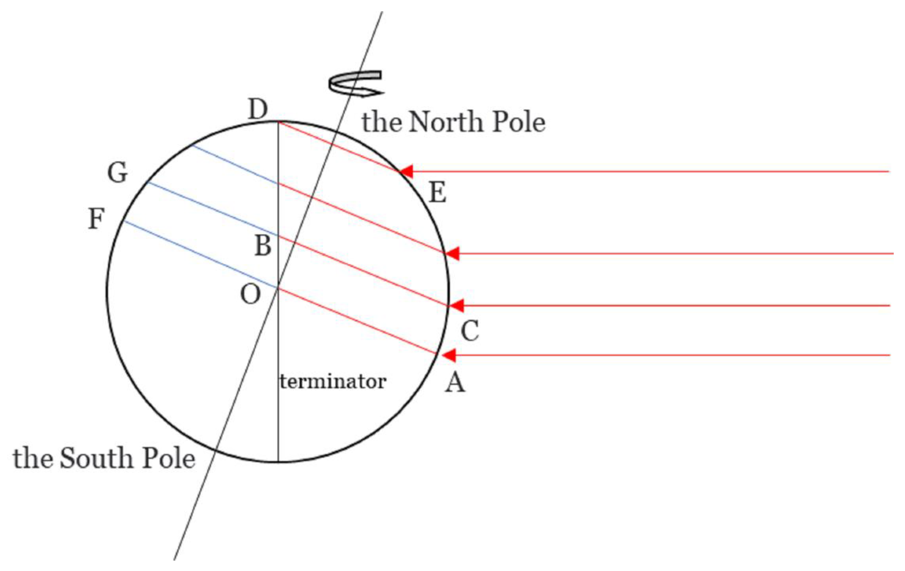
2.2.1. The Law of Revolution and Rotation of Mars
2.2.2. Calculation Model of the PSD and SASR on the Sloped Surface
2.2.3. Theoretical Equation for Calculating PSD and SASR on Rugged Terrain
- (1)
- and are the hour angle of sunrise and the hour angle of sunset on the horizontal plane, respectively. Their values, changing with the varies of points’ location and time, can be given by:Note that the above Equation applies only to </2−. There are two special cases in which the above Equation is not applicable. Correspondingly, when > +1, The phenomenon of the polar night will occur, i.e., PSD should be zero. likewise, solar radiation should also be zero; When < −1, the phenomenon of the polar day will occur, i.e., PSD should be all day [1,2].
- (2)
- Using as a sun hour angle step length, the [ should evenly be divided into n intercell. For each intercell, we consider whether solar radiation is covered by surrounding terrain at the study point. Besides, there is a time step length denoted by for each different .can be given by:n can be given by:where int ( ) is a function which can obtain the integral part of theThus intercell can be obtained:
- (3)
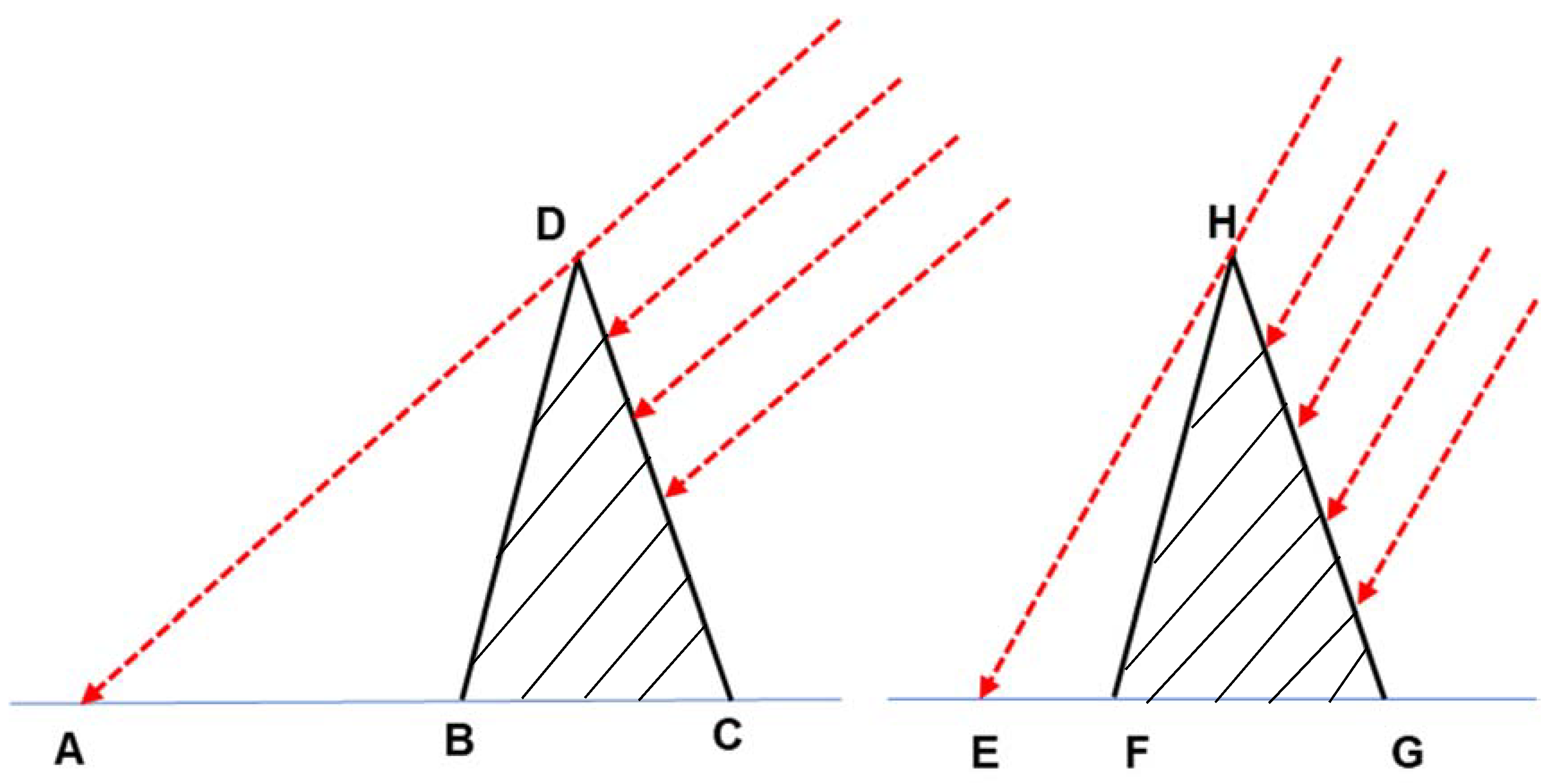
- Whether a point can be exposed to sunlight depends on the sun elevation angle and the azimuth angle and the shielding status function caused by surrounding terrain. The sun elevation angle and azimuth angle of every intercell can be given by the following Equations:where is the sun elevation angle; is the azimuth angle; Hillshade is a function of the terrain shading status depending on which we can get the terrain shading factor for each different period. we denote terrain shading status factor as where = 0 indicates the study point was shaded and = 1 indicates It was exposed to the sun.The hillshade algorithm, which was derived from and employed in the ArcGIS tool, was used to analyzes the local terrain shadow by considering the illumination source angle (solar incident angle) and surrounding terrain shadows. It is generally used to determine the assumed brightness value of a given position at a given time (solar altitude angle and solar azimuth angle vary with solar hour angle) influenced by the surrounding terrains. It has been used to determine the shielding status of solar radiation. [109,110,111,112,113,114,115,116,117].The obtained value, which was named as hillshade value, ranges from 0–255. The corresponding Equation wasThe hillshade value ranges from 0–255. When hillshade > 0, the place is incident by sun; when hillshade = 0, the place is shielded by the terrain.In this paper, the hillshade was reclassified to terrain shading status factor as according to Equation (22). When hillshade >0, = 1; when hillshade = 0, = 0.
- (4)
- We now can calculate the PSD with considering the shielding effect. The PSD considering shielding effect should be obtained by adding up all the PSD subperiod which has available sunshine. Defining as the shielding coefficient of each period which can be determined by the surrounding :The PSD of certain study point in the rugged terrains can be given by:where mod () is a function which can obtain the remainder part of the . Hereafter, the PSD indicates the PSD which considers the terrain relief.
- (5)
- The SASR which considers the terrain relief effect is obtained by adding up the SASR in all available PSD. Whether a point can be exposed to sunlight in the integral part [ is determined by the and . If = 0, = 0 or = 0, = 0, nothing should be done in the [ ; If = 0, = 1, the angle of new PSD should begin as which was the mean value of and ; If = 1, = 0, the angle of new PSD should end as which was the mean value of and . Thus, an array of solar hour angles for an m segment can be obtained (in this array, the true sunrise and sunset solar hour angle over the rugged terrains should be the beginning of the first valid PSD and the end of the last valid PSD respectively):We can obtain the daily SASR at the calculated point by adding up the SASR in the PSD which has available sunshine:where denotes the SASR for one certain Martian sol, other parameters see above.
2.2.4. Calculation of PSD and SASR for Each Martian Sol, Season, and One Year
2.3. Method for Extracting the Roughness-Mean SASR Spectrum and Roughness-Mean PSD Spectrum.
2.3.1. Extraction of Roughness
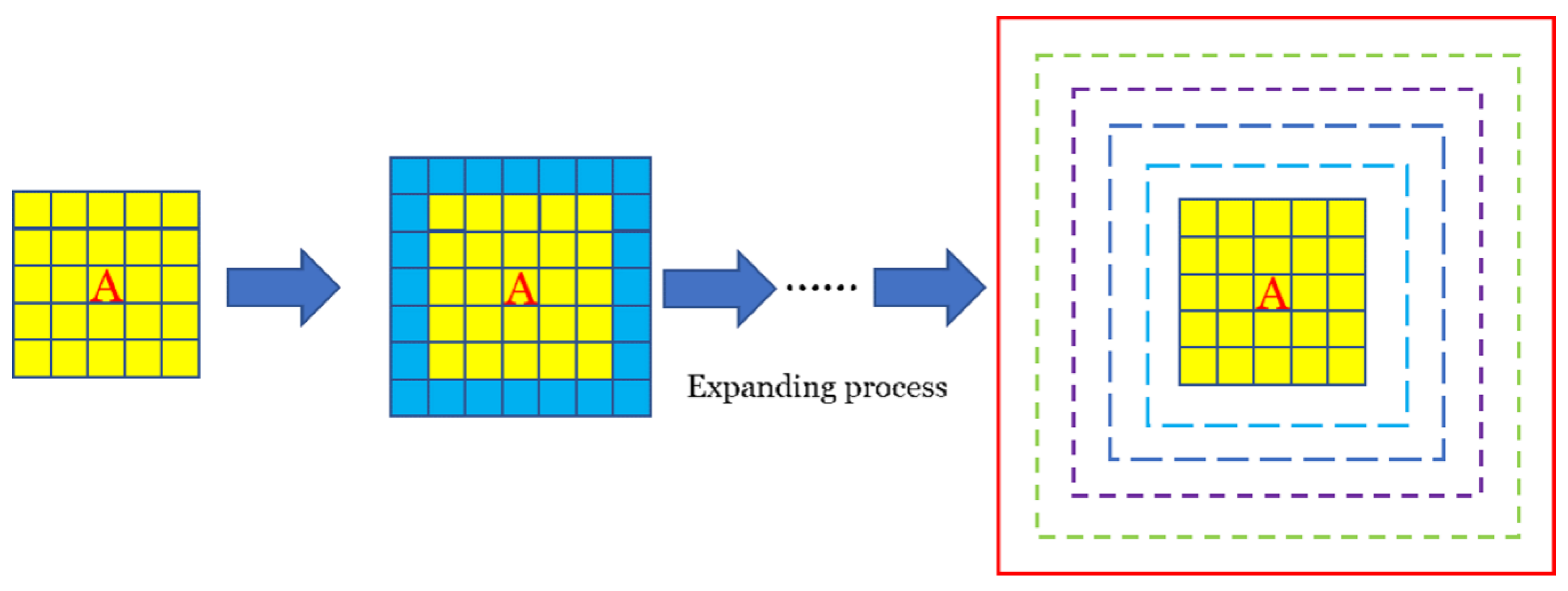
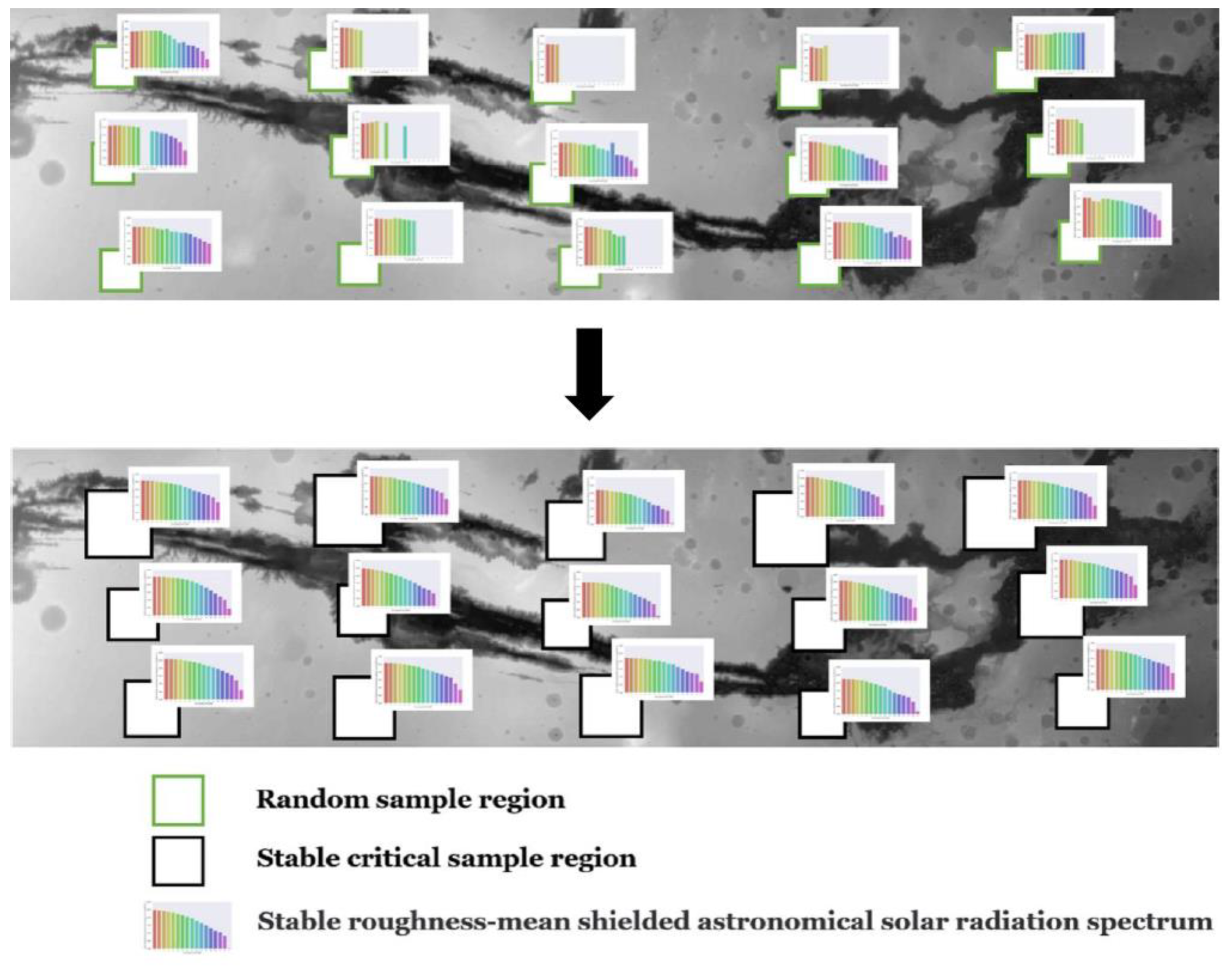
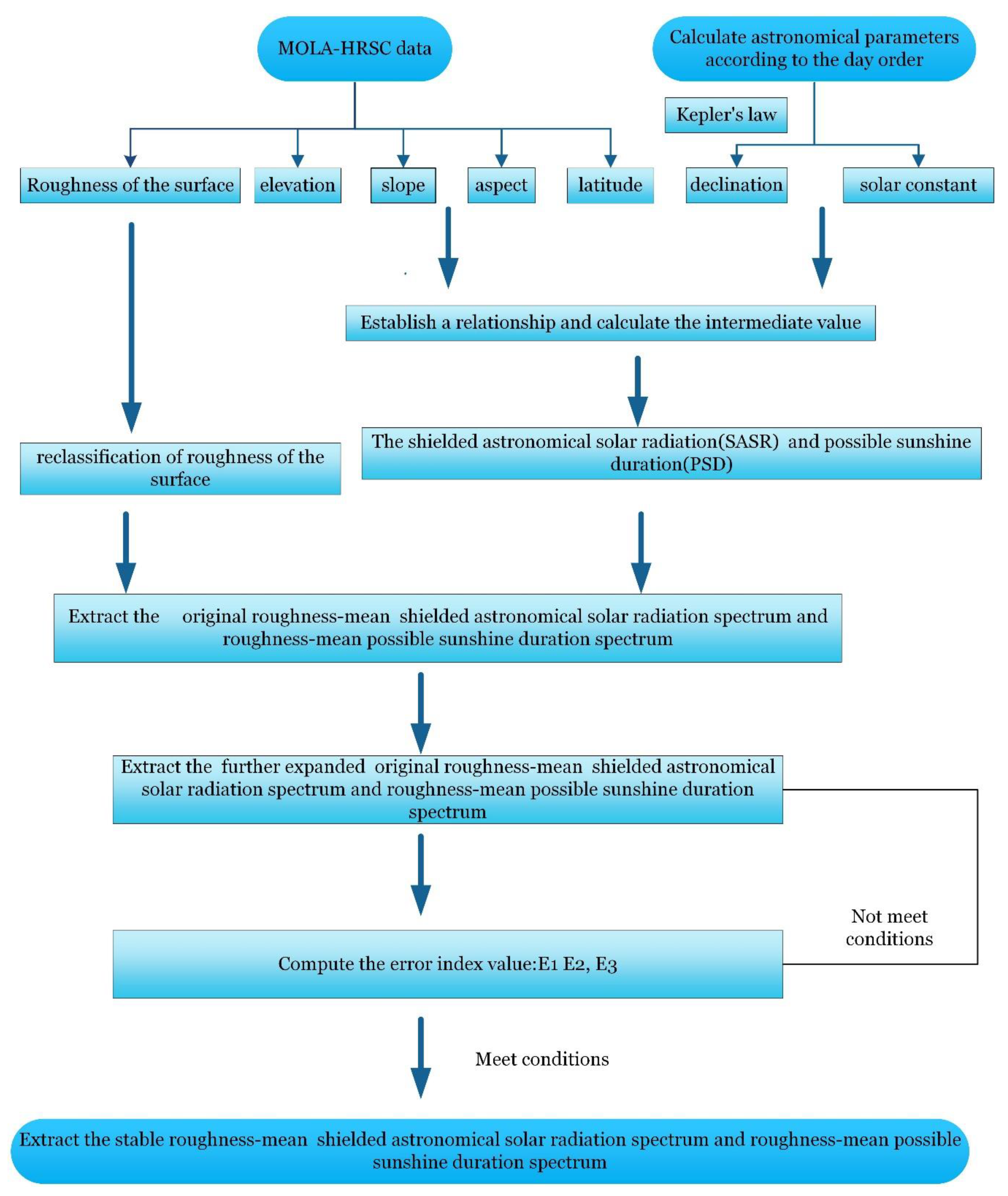
2.3.2. Extracting Procedure of the Stable Roughness-Mean Shielded Astronomical Solar Radiation Spectrum
2.3.3. Extracting Procedure of the Standard Stable Roughness-mean Shielded Astronomical Solar Radiation Spectrum
3. Results
3.1. Characteristics of Annual Spectrums
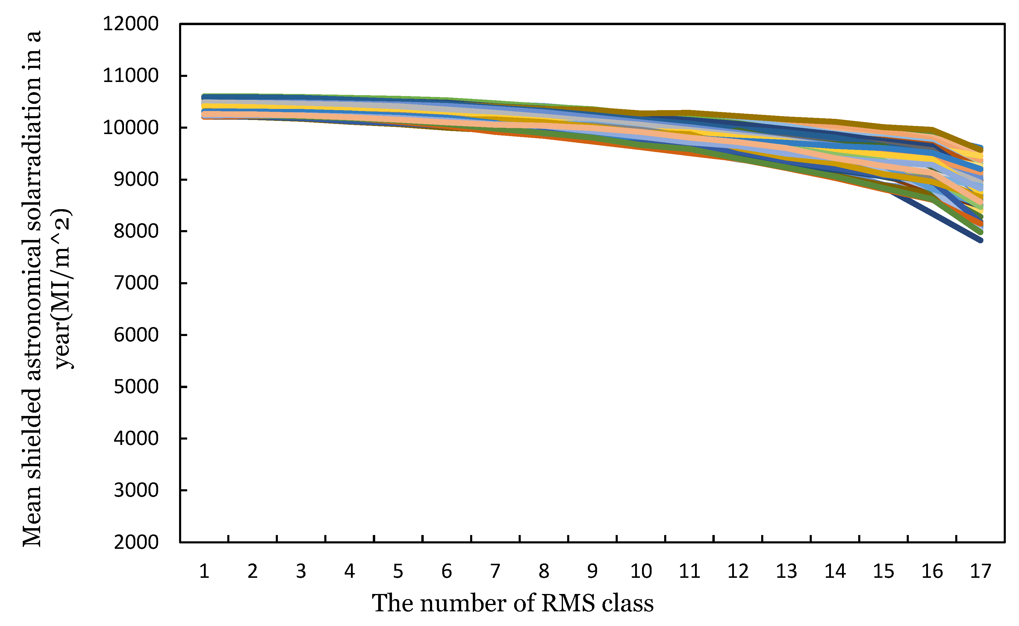
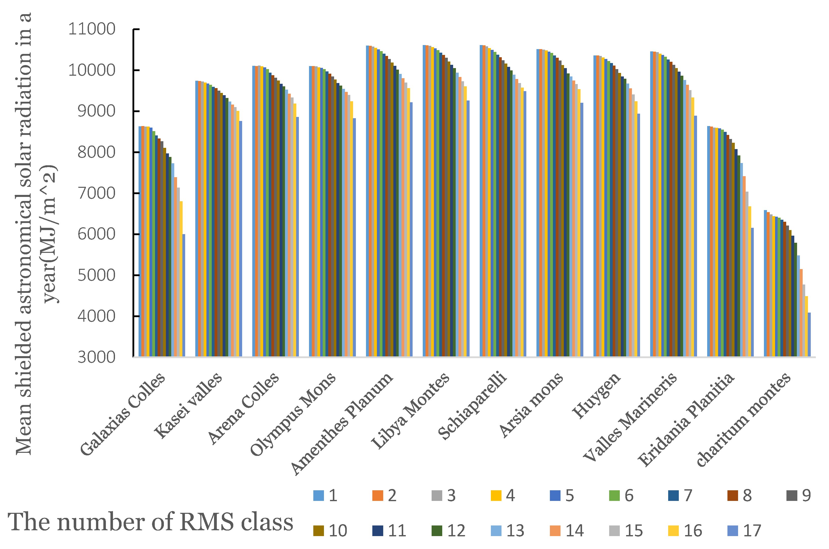
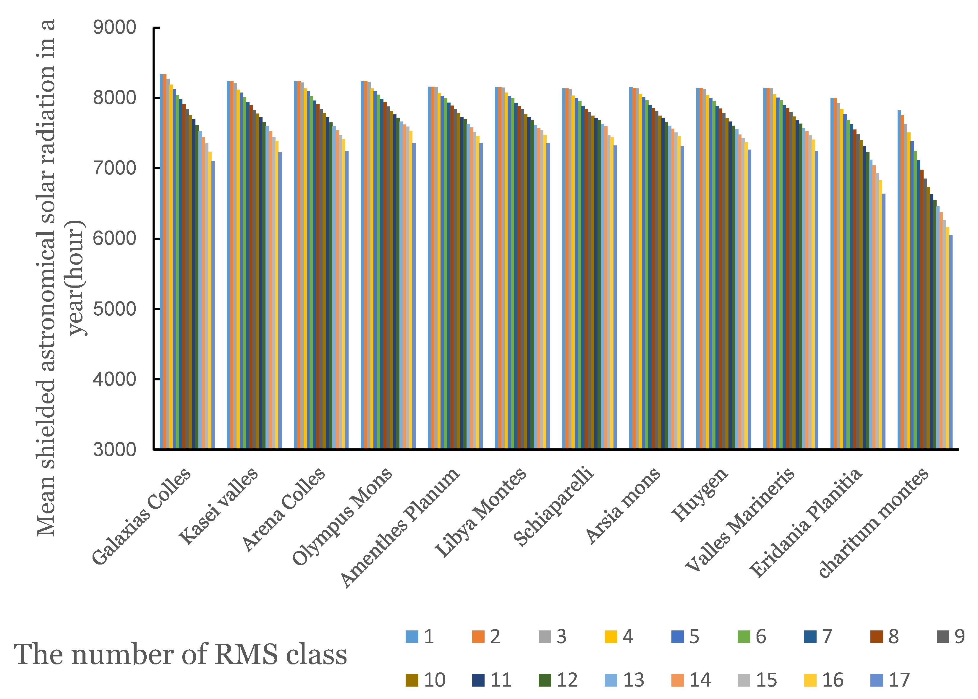
3.1.1. The Law of Gradual Variation of and with Terrain Relief in Annual Spectrum
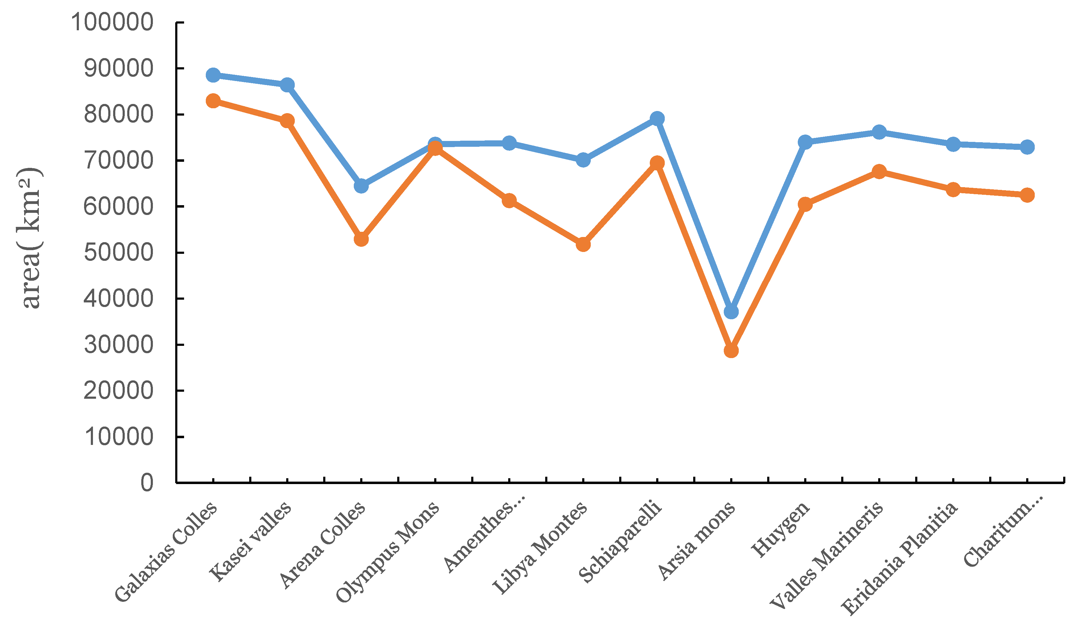
3.1.2. The Law of Critical Area with Terrain Relief
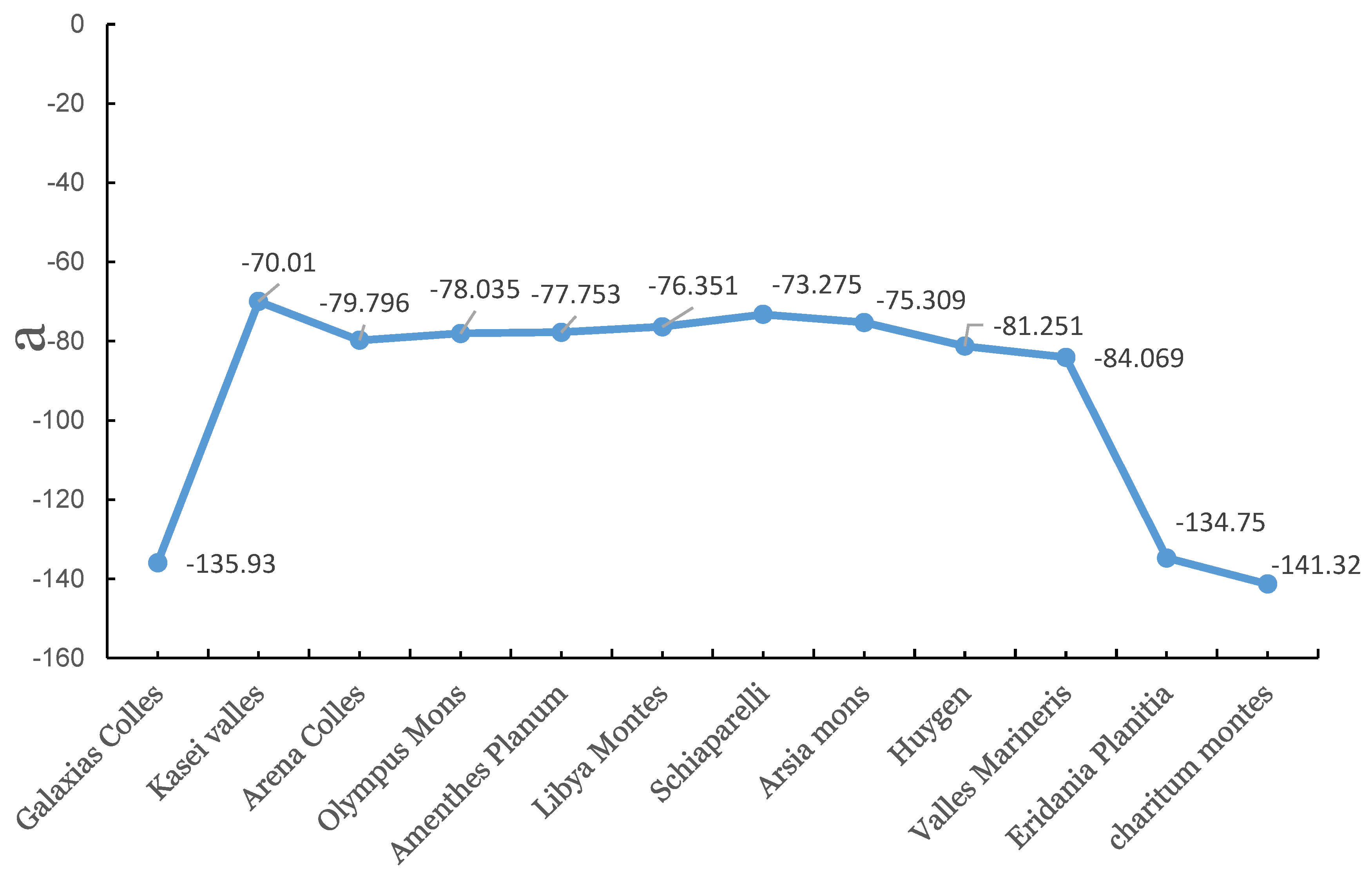
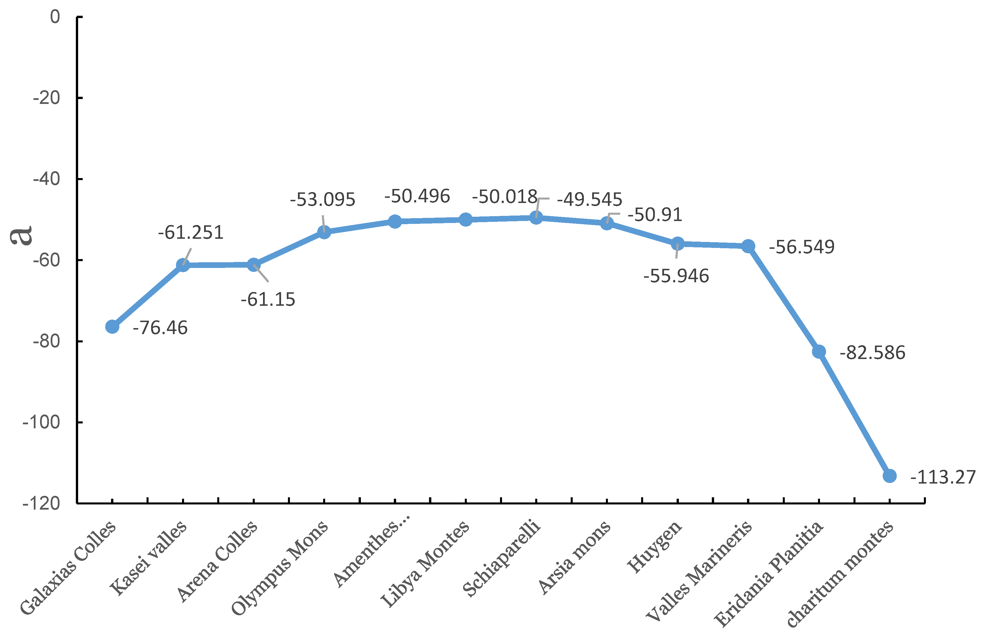
3.1.3. Latitude Anisotropy Characteristics Influenced by the Shielding Effect in and
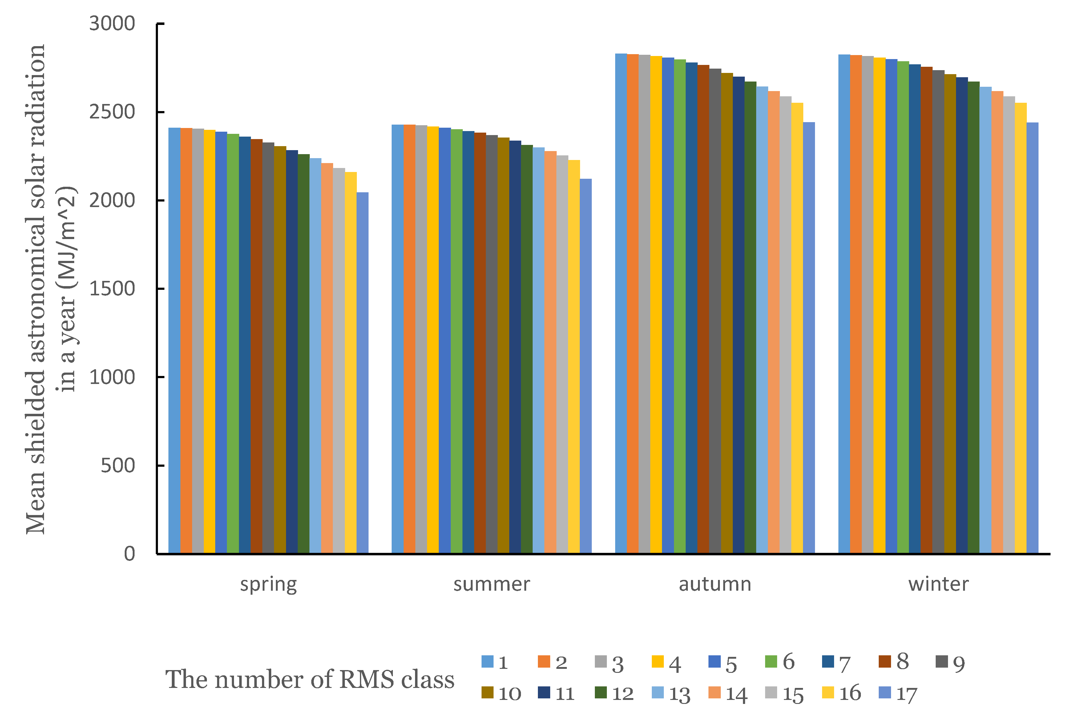
3.2. Characteristics of Spectrums in Four Seasons
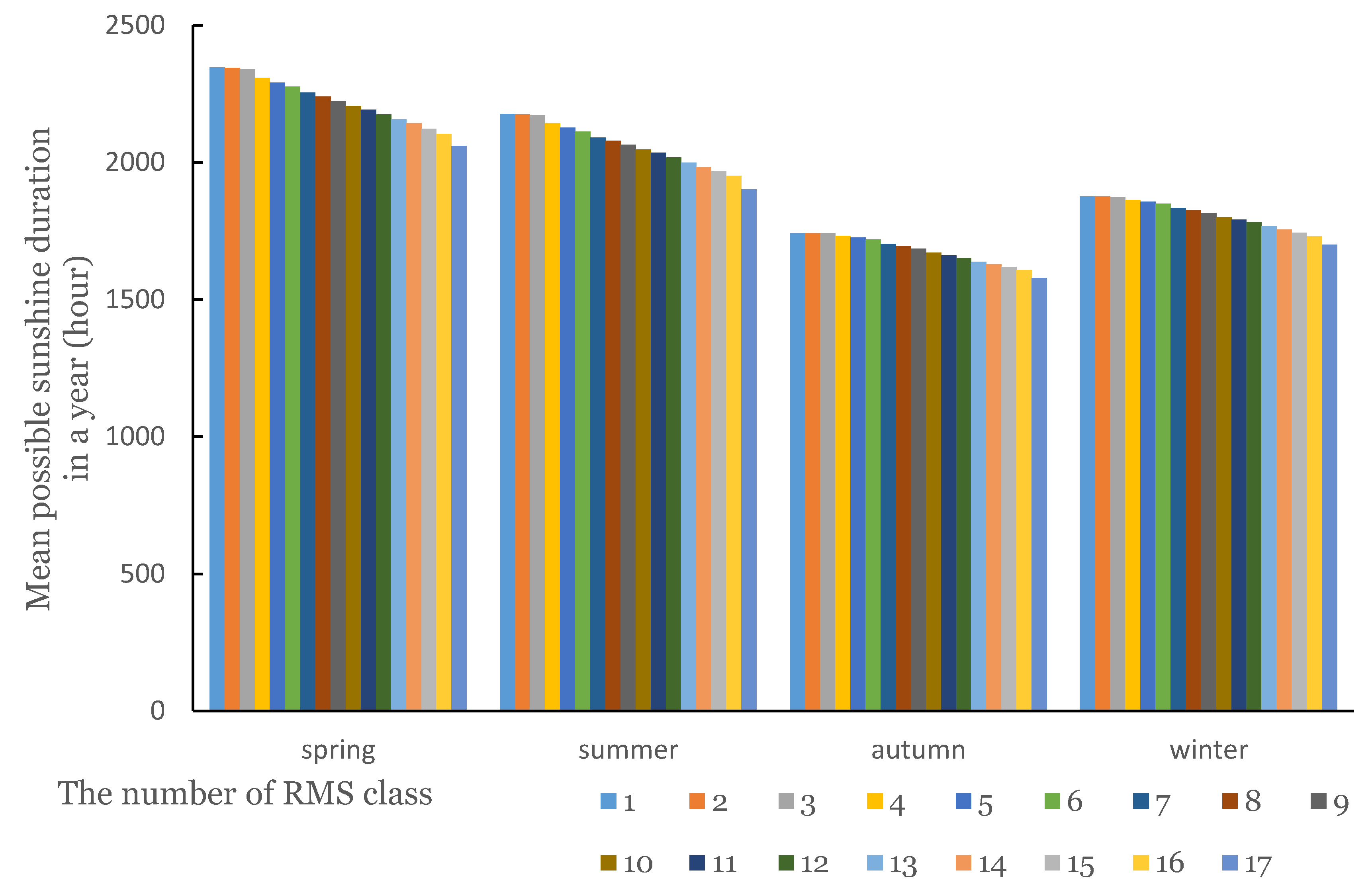
3.2.1. The Law of Gradual Variation of and with Terrain Relief in the Annual Spectrum
3.2.2. Latitude Anisotropy Characteristics Influenced by the Shielding Effect in and
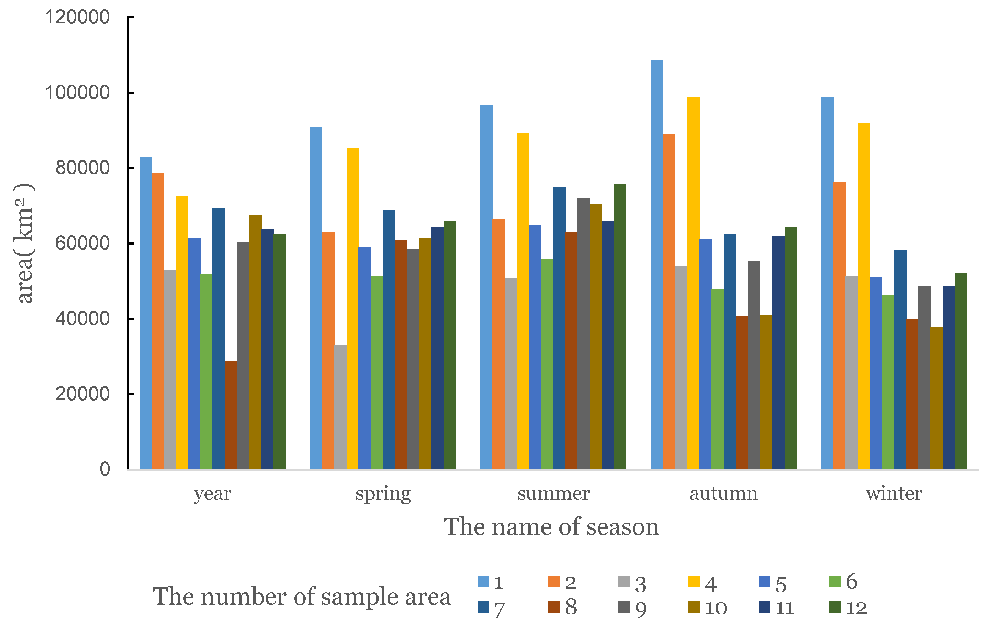
3.2.3. Relationship between Critical Areas for Spectrums in Four Seasons
4. Discussion
4.1. Discussion on the Influence of Roughness Classification Scheme on the Spectrum
4.2. The Commonalities and Differences between the Two Spectrums and Other Spectrums Proposed Before
4.2.1. Commonalities
(1) In Characteristics
(2) In Findings
4.2.2. Differences
(1) In Characteristics
(2) In Findings
4.3. Limitations
4.4. Application of this Study
5. Conclusions
- (1)
- The spectral method is a quantitative method to be more effective in identifying and characterizing the spatial-temporal distribution of SASR or PSD in sample areas. The seasonal combination spectrum in four seasons is an effective qualitative description of the temporal distribution of SASR and PSD in different landforms.
- (2)
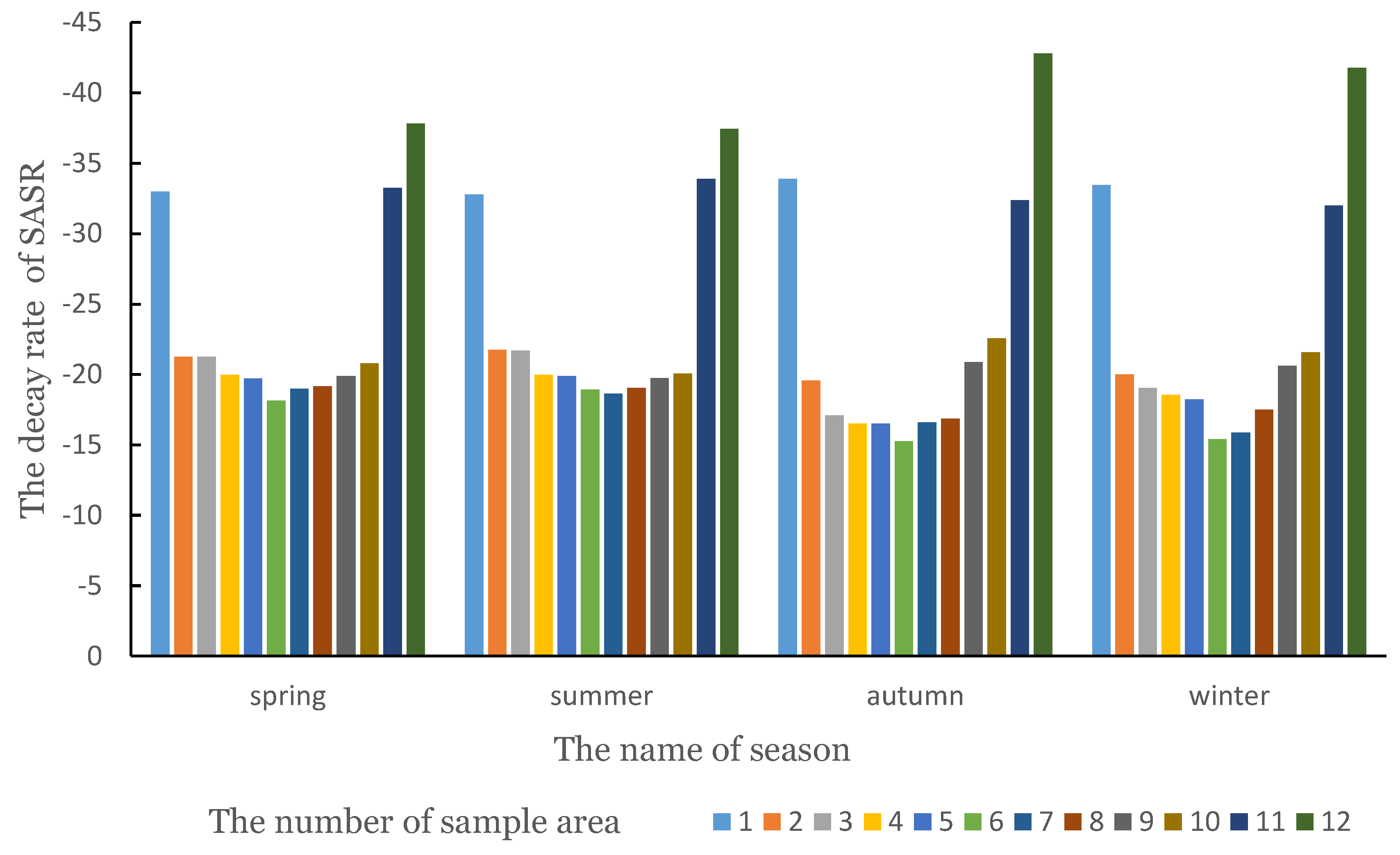
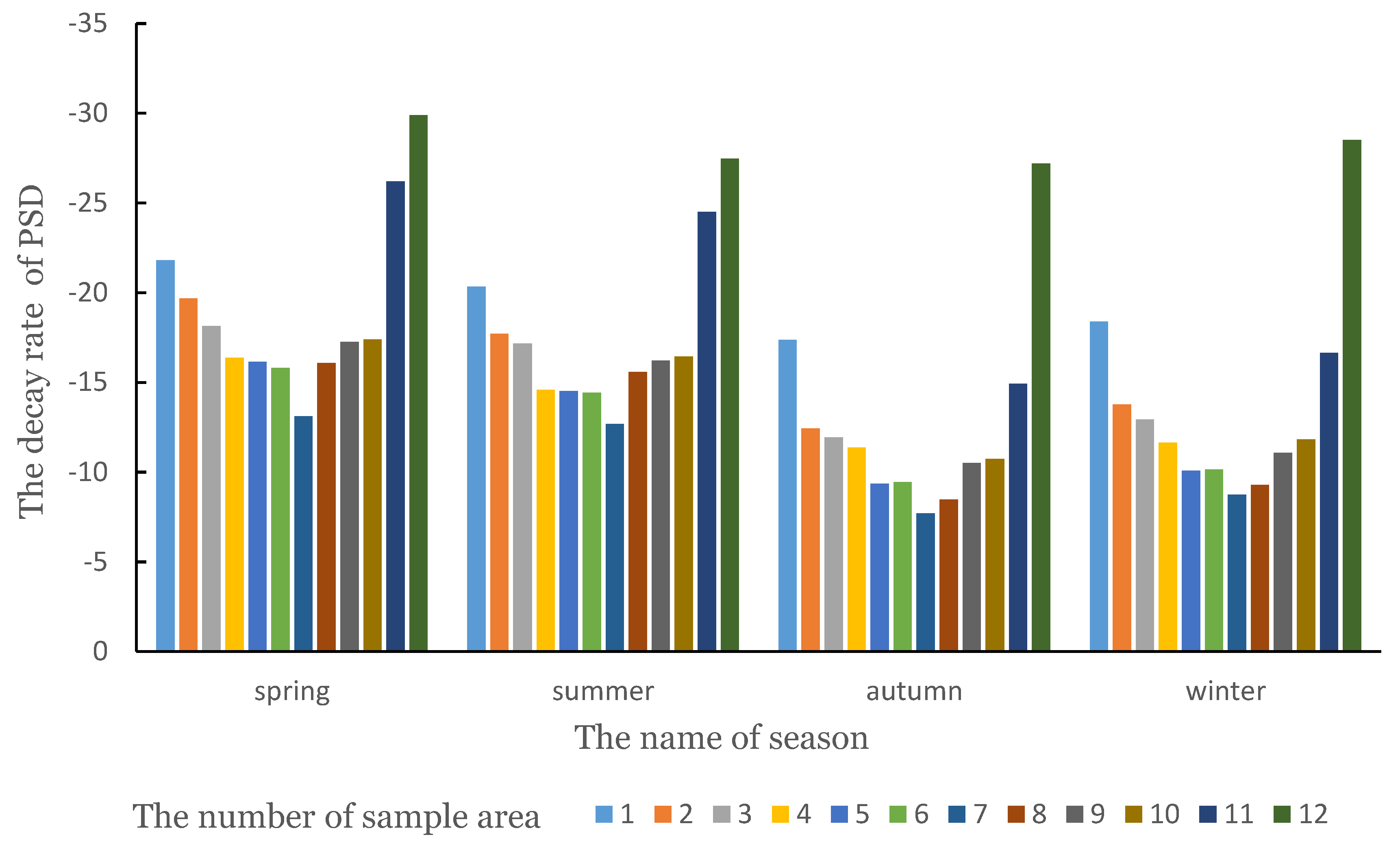
- and revealed the complex interactions between the SASR or PSD and the terrain relief. Under the terrain influences, in the and of the same landforms, the SASR and PSD showed a downward trend. This feature revealed that the SASR and PSD tended to decay under the influences of shielding effect caused by terrain relief.
- (3)
- SASR and PSD showed the latitude anisotropy characteristics. The latitude anisotropy characteristics discovered on Mars were complex and different from Earth due to the imbalanced seasons. In essence, this feature is also a manifestation of different shading effects caused by solar elevation angle.
- (4)
- SASR is more sensitive to the shielding effect than PSD which is proved by the corresponding experiments. Based on it, SASR showed more regular laws than PSD under terrain relief in a year or four seasons.
- (5)
- or can be a parameter to determine the minimum test regions for SASR or PSD of sample areas. The spatial structure of SASR or PSD become stable if the extracted region was larger than or . The relations discovered in results may help us to quickly found and test them.
Author Contributions
Funding
Data Availability Statement
Acknowledgments
Conflicts of Interest
References
- Landis, G.A. Solar radiation on mars—Stationary photovoltaic array. J. Propuls. Power 1995, 11, 554–561. [Google Scholar] [CrossRef] [Green Version]
- Appelbaum, J.; Landis, G.A.; Sherman, I. Solar radiation on Mars-Update 1991. Sol. Energy 1993, 50, 35–51. [Google Scholar] [CrossRef] [Green Version]
- Appelbaum, J.; Flood, D.J. Solar radiation on Mars. Sol. Energy 1990, 45, 353–363. [Google Scholar] [CrossRef]
- Savijärvi, H.; Crisp, D.; Harri, A.M. Effects of CO2 and dust on present-day solar radiation and climate on Mars. Q. J. R. Meteorol. Soc. 2005, 131, 2907–2922. [Google Scholar] [CrossRef]
- Monteith, J.L. Solar Radiation and Productivity in Tropical Ecosystems. J. Appl. Ecol. 1972, 9, 747–766. [Google Scholar] [CrossRef] [Green Version]
- Qiu, X.-F.; Zeng, Y.; Liu, S.-M. Distributed Modeling of Extraterrestrial Solar Radiation over Rugged Terrain. Chin. J. Geophys. 2005, 48, 1100–1107. [Google Scholar] [CrossRef]
- Whiteman, C.D.; Allwine, K.J.J.E.S. Extraterrestrial solar radiation on inclined surfaces. Environ. Softw. 1986, 1, 164–174. [Google Scholar] [CrossRef]
- Zeng, Y.; Qiu, X.; Miao, Q.; Liu, C. Distribution of possible sunshine durations over rugged terrains of China. Prog. Nat. Sci. 2003, 13, 761–764. [Google Scholar] [CrossRef]
- Vicente-Retortillo, Á.; Valero, F.; Vázquez, L.; Martínez, G.M. A model to calculate solar radiation fluxes on the Martian surface. J. Space Weather Space Clim. 2015, 5. [Google Scholar] [CrossRef] [Green Version]
- Khatib, T.; Abunajeeb, I.; Heneni, Z. Determination of Mars Solar-Belt by Modeling of Solar Radiation Using Artificial Neural Networks. J. Sol. Energy Eng. 2019, 142, 142. [Google Scholar] [CrossRef]
- Chen, N. Spectra method for revealing relations between slope and possible sunshine duration in China. Earth Sci. Inform. 2020, 13, 695–707. [Google Scholar] [CrossRef]
- Chen, N. Deriving the slope-mean shielded astronomical solar radiation spectrum and slope-mean possible sunshine duration spectrum over the Loess Plateau. J. Mt. Sci. 2020, 17, 133–146. [Google Scholar] [CrossRef]
- Marzo, A.; Trigo-Gonzalez, M.; Alonso-Montesinos, J.; Martínez-Durbán, M.; López, G.; Ferrada, P.; Fuentealba, E.; Cortés, M.; Batlles, F.J.R.E. Daily global solar radiation estimation in desert areas using daily extreme temperatures and extraterrestrial radiation. Renew. Energy 2017, 113, 303–311. [Google Scholar] [CrossRef]
- Ambreen, R.; Ahmad, I.; Qiu, X.; Li, M. Regional and Monthly Assessment of Extraterrestrial Solar Radiations in Pakistan. J. Geogr. Inf. Syst. 2015, 7, 58–64. [Google Scholar] [CrossRef] [Green Version]
- Ambreen, R.; Ahmad, I.; Qiu, X.; Li, M. Regional and Monthly Assessment of Possible Sunshine Duration in Pakistan: A Geographical Approach. J. Geogr. Inf. Syst. 2015, 7, 65–70. [Google Scholar] [CrossRef] [Green Version]
- Ahmad, M.J.; Tiwari, G.N. Solar radiation models—A review. Int. J. Energy Res. 2011, 35, 271–290. [Google Scholar] [CrossRef]
- Zeng, Y. Distributed modeling of direct solar radiation on rugged terrain of the Yellow River Basin. J. Geogr. Sci. 2005, 15, 439. [Google Scholar] [CrossRef]
- Sabo, L.M.; Mariun, N.; Hizam, H.; Radzi, M.A.M.; Zakaria, A. Estimation of solar radiation from digital elevation model in area of rough topography. World J. Eng. 2016, 13, 453–460. [Google Scholar] [CrossRef]
- Reuter, H.I.; Kersebaum, K.C.; Wendroth, O. Modelling of solar radiation influenced by topographic shading––evaluation and application for precision farming. Phys. Chem. Earth Parts A/B/C 2005, 30, 143–149. [Google Scholar] [CrossRef]
- He, Y.; Wang, K.; Zhou, C.; Wild, M. A Revisit of Global Dimming and Brightening Based on the Sunshine Duration. Geophys. Res. Lett. 2018, 45, 4281–4289. [Google Scholar] [CrossRef]
- Bazrafshan, J.; Heidari, N.; Moradi, I.; Aghashariatmadary, Z. Simultaneous stochastic simulation of monthly mean daily global solar radiation and sunshine duration hours using copulas. J. Hydrol. Eng. 2015, 20, 04014061. [Google Scholar] [CrossRef]
- Keating, K.A.; Gogan, P.J.; Vore, J.M.; Irby, L.R. A simple solar radiation index for wildlife habitat studies. J. Wildl. Manag. 2007, 71, 1344–1348. [Google Scholar] [CrossRef]
- Hanqun, S.; Baopu, F.J.A.G.S. The elliptical integralmodel of comhputing the extraterrestrial solar radiation on the slope. Acta Geogr. Sin. 1996, 6, 559–566. [Google Scholar]
- Chen, N. Scale problem: Influence of grid spacing of digital elevation model on computed slope and shielded extra-terrestrial solar radiation. Front. Earth Sci. 2020, 14, 171–187. [Google Scholar] [CrossRef]
- Appelbaum, J.; Segalov, T.; Jenkins, P.P.; Landis, G.A.; Baraona, C.R. Verification of Mars Solar Radiation Model Based on Mars Pathfinder Data. In Proceedings of the Conference Record of the Twenty Sixth IEEE Photovoltaic Specialists Conference—1997, Anaheim, CA, USA, 29 September–3 October 1997; pp. 1039–1041. [Google Scholar] [CrossRef]
- Appelbaum, J.; Steiner, A.; Landis, G.A.; Baraona, C.R.; Segalov, T. Spectral content of solar radiation on Martian surface based on Mars pathfinder. J. Propuls. Power 2001, 17, 508–516. [Google Scholar] [CrossRef]
- Badescu, V. Available solar energy and weather forecasting on mars surface. Mars Prospect. Energy Mater. Resour. 2009, 1, 25–66. [Google Scholar] [CrossRef]
- Badescu, V. Regional and seasonal limitations for Mars intrinsic ecopoiesis. Acta Astronaut. 2005, 56, 670–680. [Google Scholar] [CrossRef]
- Badescu, V. Simulation of solar cells utilization on the surface of mars. Acta Astronaut. 1998, 43, 443–453. [Google Scholar] [CrossRef]
- Badescu, V. Different strategies for maximum solar radiation collection on mars surface. Acta Astronaut. 1998, 43, 409–421. [Google Scholar] [CrossRef]
- Cockell, C.S.; Raven, J.A. Zones of photosynthetic potential on Mars and the early Earth. Icarus 2004, 169, 300–310. [Google Scholar] [CrossRef]
- Ghosh, H.R.; Bhowmik, N.C.; Hussain, M. Determining seasonal optimum tilt angles, solar radiations on variously oriented, single and double axis tracking surfaces at Dhaka. Renew. Energy 2010, 35, 1292–1297. [Google Scholar] [CrossRef]
- Kuhn, W.R.; Atreya, S.K. Solar radiation incident on the Martian surface. J. Mol. Evol. 1979, 14, 57–64. [Google Scholar] [CrossRef] [PubMed]
- Landis, G.A. Solar cell selection for Mars. IEEE Aerosp. Electron. Syst. Mag. 2000, 15, 17–21. [Google Scholar] [CrossRef]
- Levine, J.S.; Kraemer, D.R.; Kuhn, W.R. Solar radiation incident on Mars and the outer planets: Latitudinal, seasonal, and atmospheric effects. Icarus 1977, 31, 136–145. [Google Scholar] [CrossRef] [Green Version]
- Patel, M.R.; Zarnecki, J.C.; Catling, D.C. Ultraviolet radiation on the surface of Mars and the Beagle 2 UV sensor. Planet. Space Sci. 2002, 50, 915–927. [Google Scholar] [CrossRef]
- Thiemann, E.M.B.; Chamberlin, P.C.; Eparvier, F.G.; Templeman, B.; Woods, T.N.; Bougher, S.W.; Jakosky, B.M. The MAVEN EUVM model of solar spectral irradiance variability at Mars: Algorithms and results. J. Geophys. Res. Space Phys. 2017, 122, 2748–2767. [Google Scholar] [CrossRef]
- Vicente-Retortillo, Á.; Lemmon, M.T.; Martínez, G.M.; Valero, F.; Vázquez, L.; Martín, M.L. Variabilidad estacional e interanual de la radiación solar en las coordenadas de aterrizaje de Spirit, Opportunity y Curiosity. Física Tierra 2016, 28, 111–127. [Google Scholar] [CrossRef] [Green Version]
- Zeitlin, C.; Hassler, D.M.; Guo, J.; Ehresmann, B.; Wimmer-Schweingruber, R.F.; Rafkin, S.C.R.; von Forstner, J.L.F.; Lohf, H.; Berger, T.; Matthiae, D.; et al. Analysis of the Radiation Hazard Observed by RAD on the Surface of Mars During the September 2017 Solar Particle Event. Geophys. Res. Lett. 2018, 45, 5845–5851. [Google Scholar] [CrossRef] [Green Version]
- Badescu, V.; Popescu, G.; Feidt, M. Model of optimized solar heat engine operating on Mars. Energy Convers. Manag. 1999, 40, 1713–1721. [Google Scholar] [CrossRef]
- Badescu, V. Inference of atmospheric optical depth from near-surface meteorological parameters on Mars. Renew. Energy 2001, 24, 45–57. [Google Scholar] [CrossRef]
- Breus, T.K.; Krymskii, A.M.; Crider, D.H.; Ness, N.F.; Hinson, D.; Barashyan, K.K. Effect of the solar radiation in the topside atmosphere/ionosphere of Mars: Mars Global Surveyor observations. J. Geophys. Res. Space Phys. 2004, 109, 1–8. [Google Scholar] [CrossRef]
- Delgado-Bonal, A.; Martín-Torres, F.J.; Vázquez-Martín, S.; Zorzano, M.-P. Solar and wind exergy potentials for Mars. Energy 2016, 102, 550–558. [Google Scholar] [CrossRef]
- Hourdin, F. A new representation of the absorption by the CO 2 15-μm band for a Martian general circulation model. J. Geophys. Res. 1992, 97, 18319. [Google Scholar] [CrossRef]
- Keating, A.; Mohammadzadeh, A.; Nieminen, P.; Maia, D.; Coutinho, S.; Evans, H.; Pimenta, M.; Huot, J.P.; Daly, E. A model for Mars radiation environment characterization. IEEE Trans. Nucl. Sci. 2005, 52, 2287–2293. [Google Scholar] [CrossRef]
- Lee, C.O.; Jakosky, B.M.; Luhmann, J.G.; Brain, D.A.; Mays, M.L.; Hassler, D.M.; Holmström, M.; Larson, D.E.; Mitchell, D.L.; Mazelle, C.; et al. Observations and Impacts of the 10 September 2017 Solar Events at Mars: An Overview and Synthesis of the Initial Results. Geophys. Res. Lett. 2018, 45, 8871–8885. [Google Scholar] [CrossRef]
- Nagaraja, K.; Basuvaraj, P.K.; Chakravarty, S.C.; Kuttanpillai, P.K. Effect of Incoming Solar Particle Radiations on the Exosphere of Mars. arXiv 2020, arXiv:2008.10029. [Google Scholar]
- Kamsali, N.; Basuvaraj, P.K.; Chakravarty, S. Effect of Solar Radiation on Exosphere of Mars. arXiv 2020, arXiv:2008.10029. [Google Scholar] [CrossRef]
- Nakamura, T.; Tajika, E. Stability of the Martian climate system under the seasonal change condition of solar radiation. J. Geophys. Res. E Planets 2002, 107, 1–10. [Google Scholar] [CrossRef] [Green Version]
- Peterson, W.K.; Thiemann, E.M.B.; Eparvier, F.G.; Andersson, L.; Fowler, C.M.; Larson, D.; Mitchell, D.; Mazelle, C.; Fontenla, J.; Evans, J.S.; et al. Photoelectrons and solar ionizing radiation at Mars: Predictions versus MAVEN observations. J. Geophys. Res. Space Phys. 2016, 121, 8859–8870. [Google Scholar] [CrossRef]
- Pollack, J.B.; Haberle, R.M.; Murphy, J.R.; Schaeffer, J.; Lee, H. Simulations of the general circulation of the Martian atmosphere. 2. Seasonal pressure variations. J. Geophys. Res. 1993, 98, 3149–3181. [Google Scholar] [CrossRef]
- Townsend, L.W.; Pourarsalan, M.; Hall, M.I.; Anderson, J.A.; Bhatt, S.; Delauder, N.; Adamczyk, A.M. Estimates of Carrington-class solar particle event radiation exposures on Mars. Acta Astronaut. 2011, 69, 397–405. [Google Scholar] [CrossRef]
- Wolff, M.J.; Smith, M.D.; Clancy, R.T.; Arvidson, R.; Kahre, M.; Seelos Iv, F.; Murchie, S.; Savijärvi, H. Wavelength dependence of dust aerosol single scattering albedo as observed by the Compact Reconnaissance Imaging Spectrometer. J. Geophys. Res. E Planets 2009, 114, 12–13. [Google Scholar] [CrossRef]
- Zou, H.; Wang, J.S.; Nielsen, E. Reevaluating the relationship between the Martian ionospheric peak density and the solar radiation. J. Geophys. Res. 2006, 111, A07305. [Google Scholar] [CrossRef] [Green Version]
- Allison, M.; McEwen, M. A post-Pathfinder evaluation of areocentric solar coordinates with improved timing recipes for Mars seasonal/diurnal climate studies. Planet. Space Sci. 2000, 48, 215–235. [Google Scholar] [CrossRef] [Green Version]
- Madeleine, J.B.; Forget, F.; Head, J.W.; Levrard, B.; Montmessin, F.; Millour, E. Amazonian northern mid-latitude glaciation on Mars: A proposed climate scenario. Icarus 2009, 203, 390–405. [Google Scholar] [CrossRef] [Green Version]
- Qiu, X.; Zeng, Y.; Liu, C.; Wu, X. Simulation of astronomical solar radiation over Yellow River Basin based on DEM. J. Geogr. Sci. 2004, 14, 63–69. [Google Scholar] [CrossRef]
- Bennie, J.; Huntley, B.; Wiltshire, A.; Hill, M.O.; Baxter, R. Slope, aspect and climate: Spatially explicit and implicit models of topographic microclimate in chalk grassland. Ecol. Model. 2008, 216, 47–59. [Google Scholar] [CrossRef]
- Park, J.-K.; Das, A.; Park, J.-H. A new approach to estimate the spatial distribution of solar radiation using topographic factor and sunshine duration in South Korea. Energy Convers. Manag. 2015, 101, 30–39. [Google Scholar] [CrossRef]
- Piedallu, C.; Gégout, J.-C. Multiscale computation of solar radiation for predictive vegetation modelling. Ann. For. Sci. 2007, 64, 899–909. [Google Scholar] [CrossRef] [Green Version]
- Sypka, P.; Starzak, R.; Owsiak, K. Methodology to estimate variations in solar radiation reaching densely forested slopes in mountainous terrain. Int. J. Biometeorol. 2016, 60, 1983–1994. [Google Scholar] [CrossRef]
- Zhang, H.; Liu, G.; Huang, C. Modeling all-sky global solar radiation using MODIS atmospheric products: A case study in Qinghai-Tibet Plateau. Chin. Geogr. Sci. 2010, 20, 513–521. [Google Scholar] [CrossRef] [Green Version]
- Allen, R.G.; Trezza, R.; Tasumi, M. Analytical integrated functions for daily solar radiation on slopes. Agric. For. Meteorol. 2006, 139, 55–73. [Google Scholar] [CrossRef]
- Ambreen, R.; Qiu, X.; Ahmad, I. Distributed modeling of extraterrestrial solar radiation over the rugged terrains of Pakistan. J. Mt. Sci. 2011, 8, 427–436. [Google Scholar] [CrossRef]
- Nettesheim, F.C.; Conto, T.d.; Pereira, M.G.; Machado, D.L. Contribution of Topography and Incident Solar Radiation to Variation of Soil and Plant Litter at an Area with Heterogeneous Terrain. Rev. Bras. Ciência 2015, 39, 750–762. [Google Scholar] [CrossRef] [Green Version]
- Manara, V.; Beltrano, M.C.; Brunetti, M.; Maugeri, M.; Sanchez-Lorenzo, A.; Simolo, C.; Sorrenti, S. Sunshine duration variability and trends in Italy from homogenized instrumental time series (1936–2013). J. Geophys. Res. 2015, 120, 3622–3641. [Google Scholar] [CrossRef]
- Manara, V.; Brunetti, M.; Maugeri, M.; Sanchez-Lorenzo, A.; Wild, M. Sunshine duration and global radiation trends in Italy (1959-2013): To what extent do they agree? J. Geophys. Res. 2017, 122, 4312–4331. [Google Scholar] [CrossRef]
- Tsekouras, G.; Koutsoyiannis, D. Stochastic analysis and simulation of hydrometeorological processes associated with wind and solar energy. Renew. Energy 2014, 63, 624–633. [Google Scholar] [CrossRef]
- Hemelrijck, E. The effect of orbital element variations on the mean seasonal daily insolation on Mars. Moon Planets 1983, 28, 125–136. [Google Scholar] [CrossRef]
- Kolb, C.; Abart, R.; Bérces, A.; Garry, J.R.C.; Hansen, A.A.; Hohenau, W.; Kargl, G.; Lammer, H.; Patel, M.R.; Rettberg, P.; et al. An ultraviolet simulator for the incident Martian surface radiation and its applications. Int. J. Astrobiol. 2005, 4, 241–249. [Google Scholar] [CrossRef] [Green Version]
- Ogibalov, V.P.; Shved, G.M. An improved model of radiative transfer for the NLTE problem in the NIR bands of CO2 and CO molecules in the daytime atmosphere of Mars. 1. Input data and calculation method. Sol. Syst. Res. 2016, 50, 316–328. [Google Scholar] [CrossRef]
- Ono, E.; Cuello, J.L. Photosynthetically active radiation (PAR) on Mars for advanced life support. SAE Tech. Pap. 2000, 1–8. [Google Scholar] [CrossRef]
- Cord, A.; Baratoux, D.; Mangold, N.; Martin, P.; Pinet, P.; Greeley, R.; Costard, F.; Masson, P.; Foing, B.; Neukum, G. Surface roughness and geological mapping at subhectometer scale from the High Resolution Stereo Camera onboard Mars Express. Icarus 2007, 191, 38–51. [Google Scholar] [CrossRef]
- Kreslavsky, M.A.; Head, J.W. Kilometer-scale roughness of Mars: Results from MOLA data analysis. J. Geophys. Res. Planets 2000, 105, 26695–26711. [Google Scholar] [CrossRef]
- Guo, T.; Yang, X. ArcGIS Spatial Analysis Experiment Tutorial; Science Press: Beijing, China, 2006; Volume 196. (In Chinese) [Google Scholar]
- Li, F.; Tang, G.; Wang, C.; Cui, L.; Zhu, R. Slope spectrum variation in a simulated loess watershed. Front. Earth Sci. 2016, 10, 328–339. [Google Scholar] [CrossRef]
- Li, F.; Tang, G.; Wang, C.; Zhang, T. Quantitative analysis and spatial distribution of slope spectrum: A case study in the Loess Plateau in north Shaanxi province. Geospat. Inf. Sci. 2007, 6753, 67531R. [Google Scholar] [CrossRef]
- Tang, G.; Song, X.; Li, F.; Zhang, Y.; Xiong, L. Slope spectrum critical area and its spatial variation in the Loess Plateau of China. J. Geogr. Sci. 2015, 25, 1452–1466. [Google Scholar] [CrossRef] [Green Version]
- Tang, G.A.; Li, F.Y.; Liu, X.J.; Long, Y.; Yang, X. Research on the slope spectrum of the Loess Plateau. Sci. China Ser. E Technol. Sci. 2008, 51, 175–185. [Google Scholar] [CrossRef]
- Wang, C.; Tang, G.; Li, F.; Yang, X.; Ge, S.-S. Fundamental conditions of slope spectrum abstraction and application. Sci. Geogr. Sin. 2007, 27, 587. [Google Scholar]
- Orosei, R. Self-affine behavior of Martian topography at kilometer scale from Mars Orbiter Laser Altimeter data. J. Geophys. Res. 2003, 108, 8023. [Google Scholar] [CrossRef]
- Rodrigue, C. Geography of Mars. California Map Society Conference, Long Beach, CA, November; Science Press: Beijing, China, 2014; Available online: https://web.csulb.edu/~rodrigue/mars/cms14/ (accessed on 27 January 2021).
- Sheehan, W. Camille Flammarion’s the Planet Mars; Springer: New York, NA, USA, 2015; pp. 435–441. [Google Scholar] [CrossRef]
- Bourke, M.C.; Balme, M.; Beyer, R.A.; Williams, K.K.; Zimbelman, J. A comparison of methods used to estimate the height of sand dunes on Mars. Geomorphology 2006, 81, 440–452. [Google Scholar] [CrossRef]
- Caldarelli, G.; De Los Rios, P.; Montuori, M.; Servedio, V.D.P. Statistical features of drainage basins in mars channel networks. Eur. Phys. J. B Condens. Matter Complex. Syst. 2004, 38, 387–391. [Google Scholar] [CrossRef]
- Chapman, M.G.; Allen, C.C.; Gudmundsson, M.T.; Gulick, V.C.; Jakobsson, S.P.; Lucchitta, B.K.; Skilling, I.P.; Waitt, R.B. Volcanism and Ice Interactions on Earth and Mars; Springer: Boston, MA, USA, 2000; pp. 39–73. [Google Scholar] [CrossRef]
- Hare, T.M.; Skinner, J., Jr.; Liszewski, E.; Tanaka, K.; Barlow, N.G. Mars Crater Density Tools: Project Report. In Proceedings of the 37th Annual Lunar and Planetary Science Conference, League City, TX, USA, 13–17 March 2006; p. 2398. [Google Scholar]
- Li, C.; Dong, Z.; Lü, P.; Zhao, J.; Fu, S.; Feng, M.; Zhu, C. A morphological insight into the Martian dune geomorphology. Chin. Sci. Bull. 2019, 65, 80–90. [Google Scholar] [CrossRef]
- Li, J.; Cao, W.; Tian, X. Topographic surface roughness analysis based on image processing of terrestrial planet. Clust. Comput. 2019, 22, 8689–8702. [Google Scholar] [CrossRef]
- Badescu, V. Mars: Prospective Energy and Material Resources; Springer Science & Business Media: Berlin/Heidelberg, Germany, 2009. [Google Scholar]
- O’Gallagher, J.J.; Simpson, J.A. Search for trapped electrons and a magnetic moment at Mars by Mariner IV. Science 1965, 149, 1233–1239. [Google Scholar] [CrossRef]
- Ward, W.R. Present obliquity oscillations of Mars: Fourth-order accuracy in orbital e and I. J. Geophys. Res. Solid Earth 1979, 84, 237–241. [Google Scholar] [CrossRef]
- Laskar, J.; Correia, A.C.M.; Gastineau, M.; Joutel, F.; Levrard, B.; Robutel, P. Long term evolution and chaotic diffusion of the insolation quantities of Mars. Icarus 2004, 170, 343–364. [Google Scholar] [CrossRef] [Green Version]
- Li, X.; Cheng, G.; Chen, X.; Lu, L. Modification of solar radiation model over rugged terrain. Chin. Sci. Bull. 1999, 44, 1345–1349. [Google Scholar] [CrossRef]
- Zhang, J.; Zhao, L.; Deng, S.; Xu, W.; Zhang, Y. A critical review of the models used to estimate solar radiation. Renew. Sustain. Energy Rev. 2017, 70, 314–329. [Google Scholar] [CrossRef]
- Wang, S. Study on astronomical solar radiation over rugged terrain using DEM data. In Proceedings of the 2009 First International Conference on Information Science and Engineering, Nanjing, China, 26–28 December 2009; pp. 2184–2187. [Google Scholar] [CrossRef]
- Romana, A.; Xinfa, Q.; Ahmad, I.; Sultan, S. Impact of landforms on the spatial distribution of extraterrestrial solar radiation in the months of March and September: A geographical approach. Pak. J. Meteorol. 2012, 9, 1–9. [Google Scholar]
- Qiu, X.-F.; Zeng, Y.; He, Y.-J.; Liu, C.-M. Distributed Modeling of Diffuse Solar Radiation over Rugged Terrain of the Yellow River Basin. Chin. J. Geophys. 2008, 51, 700–708. [Google Scholar] [CrossRef]
- Wang, L.; Qiu, X.; Wang, P.; Wang, X.; Liu, A. Influence of complex topography on global solar radiation in the Yangtze River Basin. J. Geogr. Sci. 2014, 24, 980–992. [Google Scholar] [CrossRef] [Green Version]
- Wilson, J. Mountain Environments and Geographic Information Systems. N Z Geogr 1996, 52, 50. [Google Scholar] [CrossRef]
- Alvioli, M.; Marchesini, I.; Melelli, L.; Guth, P. Geomorphometry 2020 Conference Proceedings; CNR Edizioni: Perugia, Italy, 2020; Available online: https://www.researchgate.net/publication/343537333_Geomorphometry_2020_conference_proceedings (accessed on 27 January 2021). [CrossRef]
- Kalogirou, S. Environmental Characteristics. In Solar Energy Engineering; Elsevier: Amsterdam, The Netherlands, 2009; pp. 49–762. [Google Scholar] [CrossRef]
- Schmude, R., Jr. The North Polar Cap of Mars. Ga. J. Sci. 2014, 72, 1. [Google Scholar]
- Lowell, P.; Slipher, E. Position of the axis of Mars. Astron. Nachr. 1908, 178. [Google Scholar] [CrossRef]
- Harvey, D. The Analemmas of the Planets. Sky Telescope. 1982, 6, 237. [Google Scholar]
- Forget, F.; Montmessin, F.; Bertaux, J.L.; González-Galindo, F.; Lebonnois, S.; Quémerais, E.; Reberac, A.; Dimarellis, E.; López-Valverde, M.A. Density and temperatures of the upper Martian atmosphere measured by stellar occultations with Mars Express SPICAM. J. Geophys. Res. E Planets 2009, 114, 1–19. [Google Scholar] [CrossRef] [Green Version]
- Goddard, N. Accurate analytic representations of solar time and seasons on Mars with applications to the Pathfinder / Surveyor missions mean sun implies a Mars tropical orbit period s L s—• FractionalPart [1 + FractionalPart [Ls]] 360 (O • s) really Tropical Y. Geophys. Res. Lett. 1997, 24, 1967–1970. [Google Scholar]
- Newman, C.E.; Lewis, S.R.; Read, P.L. The atmospheric circulation and dust activity in different orbital epochs on Mars. Icarus 2005, 174, 135–160. [Google Scholar] [CrossRef] [Green Version]
- Hong, T.; Lee, M.; Koo, C.; Jeong, K.; Kim, J. Development of a method for estimating the rooftop solar photovoltaic (PV) potential by analyzing the available rooftop area using Hillshade analysis. Appl. Energy 2017, 194, 320–332. [Google Scholar] [CrossRef]
- Corripio, J.G. Vectorial algebra algorithms for calculating terrain parameters from dems and solar radiation modelling in mountainous terrain. Int. J. Geogr. Inf. Sci. 2003, 17, 1–23. [Google Scholar] [CrossRef]
- Kumar, L.; Skidmore, A.K.; Knowles, E. Modelling topographic variation in solar radiation in a GIS environment. Int. J. Geogr. Inf. Sci. 1997, 11, 475–497. [Google Scholar] [CrossRef]
- Najafifar, A.; Hosseinzadeh, J.; Karamshahi, A. The Role of Hillshade, Aspect, and Toposhape in the Woodland Dieback of Arid and Semi-Arid Ecosystems: A Case Study in Zagros Woodlands of Ilam Province, Iran. J. Landsc. Ecol. 2019, 12. [Google Scholar] [CrossRef] [Green Version]
- Zhang, S.; Li, X.; She, J. Error assessment of grid-based terrain shading algorithms for solar radiation modeling over complex terrain. Trans. GIS 2019, 24, 230–252. [Google Scholar] [CrossRef]
- Serebryakova, M.; Veronesi, F.; Hurni, L. Sine Wave, Clustering and Watershed Analysis to Implement Adaptive Illumination and Generalisation in Shaded Relief Representations. In Proceedings of the 27th International Cartographic Conference, Rio de Janeiro, Brazil, 23–28 August 2015. [Google Scholar]
- Hong, T.; Lee, M.; Koo, C.; Kim, J.; Jeong, K. Estimation of the Available Rooftop Area for Installing the Rooftop Solar Photovoltaic (PV) System by Analyzing the Building Shadow Using Hillshade Analysis. Energy Procedia 2016, 88, 408–413. [Google Scholar] [CrossRef] [Green Version]
- McDonnell, R.; Lloyd, C.; Burrough, P. Principles of Geographical Information Systems; Oxford University Press: Oxford, UK, 2015; pp. 7–17. [Google Scholar]
- Pro, A. ArcGIS for Desktop. 2018. Available online: http://pro.arcgis.com/en/pro-app/toolreference/spatial (accessed on 1 December 2020).
- Chang, K.-t.; Tsai, B.-w. The Effect of DEM Resolution on Slope and Aspect Mapping. Cartogr. Geogr. Inf. Syst. 2013, 18, 69–77. [Google Scholar] [CrossRef]
- Aharonson, O.; Zuber, M.; Rothman, D. Statistics of Mars’ topography from the Mars Orbiter Laser Altimeter: Slopes, correlations, and physical models. J. Geophys. Res. Planets 2001, 106, 23723–23735. [Google Scholar] [CrossRef]
- Beyer, R.A.; Kirk, R.L. Meter-scale slopes of candidate MSL landing sites from point photoclinometry. Space Sci. Rev. 2012, 170, 775–791. [Google Scholar] [CrossRef]
- Garvin, J.; Frawley, J. Global Vertical Roughness of Mars from Mars Orbiter Laser Altimeter Pulse-Width Measurements; Lunar and Planetary Science; 2000; Available online: https://www.researchgate.net/publication/4673801_Global_Vertical_Roughness_of_Mars_from_Mars_Orbiter_Laser_Altimeter_Pulse-Width_Measurements (accessed on 27 January 2021).
- Kreslavsky, M.A.; Head, J.W. Kilometer-scale slopes on Mars and their correlation with geologic units: Initial results from Mars Orbiter Laser Altimeter (MOLA) data. J. Geophys. Res. Planets 1999, 104, 21911–21924. [Google Scholar] [CrossRef]
- Neumann, G.A. Mars Orbiter Laser Altimeter pulse width measurements and footprint-scale roughness. Geophys. Res. Lett. 2003, 30, 1561. [Google Scholar] [CrossRef]
- Rosenburg, M.A.; Aharonson, O.; Head, J.W.; Kreslavsky, M.A.; Mazarico, E.; Neumann, G.A.; Smith, D.E.; Torrence, M.H.; Zuber, M.T. Global surface slopes and roughness of the Moon from the Lunar Orbiter Laser Altimeter. J. Geophys. Res. E Planets 2011, 116, 1–11. [Google Scholar] [CrossRef] [Green Version]
- Shepard, M.K.; Campbell, B.A.; Bulmer, M.H.; Farr, T.G.; Gaddis, L.R.; Plaut, J.J. The roughness of natural terrain: A planetary and remote sensing perspective. J. Geophys. Res. Planets 2001, 106, 32777–32795. [Google Scholar] [CrossRef]
- Hobson, R.D. Surface Roughness in Topography: Quantitative Approach; 1972; pp. 221–245. Available online: https://oceanrep.geomar.de/37452/ (accessed on 27 January 2021). [CrossRef]
- Day, M.J. Surface roughness as a discriminator of tropical karst styles. Z. Geomorphol. 2011, 32, 1–8. [Google Scholar]
- Jones, M.P.; Yoshida, R.K. Fortran Iv Program to Determine the Proper Sequence of Records in a Datafile. Educ. Psychol. Meas. 1975, 35, 729–731. [Google Scholar] [CrossRef]
- Olaya, V. Chapter 6 Basic Land-Surface Parameters. Dev. Soil Sci. 2009, 33, 141–169. [Google Scholar]
- Hengl, T.; Reuter, H. Geomorphometry: Concepts, software, applications. Dev. Soil Sci. 2009, 33, 722. [Google Scholar]
- Anderson, F.S.; Haldeman, A.F.C.; Bridges, N.T.; Golombek, M.P.; Parker, T.J.; Neumann, G. Analysis of MOLA data for the Mars Exploration Rover landing sites. J. Geophys. Res. E Planets 2003, 108. [Google Scholar] [CrossRef]
- Tao, J.Y.; Tang, G.A.; Wang, C.; Yang, X. Evaluation of terrain roughness model based on semantic and profile feature matching. Geogr. Res. 2011, 30, 1066–1076. (In Chinese) [Google Scholar]
- Zhu, M.; Li, F.Y. Influence of slope classification on slope spectrum. Sci. Surv. Mapp. 2009, 34, 165–167. [Google Scholar]


| Sample Areas | Center Longitude | Center Latitude | Landform |
|---|---|---|---|
| Galaxias Colles | 347.78° | 39.07° | Colina |
| Kasei Valles | 297.12° | 25.14° | Vallis |
| Arena Colles | 82.93° | 24.63° | Colina |
| Olympus Mons | 226.2° | 18.65° | Volcanoes |
| Amenthes Plalatumn | 105.92° | 3.4° | Plateau |
| Libya Montes | 88.23° | 1.44° | mountain range |
| schiaparelli | 16.77° | −2.71° | impact craters |
| Arsia Mons | 239.91° | −8.26° | volcanoes |
| Huygen | 55.58° | −13.88° | impact craters |
| Valles Marineris | 301.41° | −14.01° | vallis |
| Eridania Planitia | 122.21° | −38.15° | planitia |
| Charitum Montes | 319.71° | −58.1° | mountain range |
| Month Number | Solar Longitude Range (in Degree) | Duration (in Sols) |
|---|---|---|
| 1 | 0–30 | 61 |
| 2 | 30–60 | 66 |
| 3 | 60–90 | 66 |
| 4 | 90–120 | 65 |
| 5 | 120–150 | 60 |
| 6 | 150–180 | 54 |
| 7 | 180–210 | 50 |
| 8 | 210–240 | 46 |
| 9 | 240–270 | 47 |
| 10 | 270–300 | 47 |
| 11 | 300–330 | 51 |
| 12 | 330–360 | 56 |
| Sample Area | Center Latitutde | Descending Order of Mean Maxinum Daily PSD | Descending Order of Mean Daily Shielding Effect | Descending Order of Mean Daily PSD | Descending Order of Mean PSD | Descending Order of PSD (in within Each Roughness Claass) | Descending Order of SASR (in within Each Roughness Claass) |
|---|---|---|---|---|---|---|---|
| schiaparelli | −2.71° | C, D, A, B | B, A, C, D | B, A, D, C | A, B, D, C | A, B, D, C | C, D, B, A |
| Arsia mons | −8.61° | C, D, A, B | B, A, C, D | B, A, D, C | A, B, D, C | A, B, D, C | C, D, B, A |
| Huygens | −13.88° | C, D, A, B | B, A, C, D | C, D, A, B | A, B, D, C | A, B, D, C | C, D, B, A |
| Valles Marineris | −14.01° | C, D, A, B | B, A, C, D | C, D, A, B | A, B, D, C | A, B, D, C | C, D, B, A |
| North of the Hellas Plain | −34° | C, D, A, B | B, A, C, D | C, D, A, B | D, C, A, B | C, D, B, A | |
| Eridania Planitia | −38.15° | C, D, A, B | B, A, C, D | C, D, A, B | D, A, C, B | D, A, C, B | C, D, B, A |
| South of the Hellas Plain | −48.75° | C, D, A, B | B, A, C, D | C, D, A, B | D, C, A, B | C, D, B, A | |
| charitum montes | −58.1° | C, D, A, B | B, A, C, D | C, D, A, B | D, C, A, B | D, C, A, B | C, D, B, A |
Publisher’s Note: MDPI stays neutral with regard to jurisdictional claims in published maps and institutional affiliations. |
© 2021 by the authors. Licensee MDPI, Basel, Switzerland. This article is an open access article distributed under the terms and conditions of the Creative Commons Attribution (CC BY) license (http://creativecommons.org/licenses/by/4.0/).
Share and Cite
Lin, S.; Chen, N. DEM Based Study on Shielded Astronomical Solar Radiation and Possible Sunshine Duration under Terrain Influences on Mars by Using Spectral Methods. ISPRS Int. J. Geo-Inf. 2021, 10, 56. https://0-doi-org.brum.beds.ac.uk/10.3390/ijgi10020056
Lin S, Chen N. DEM Based Study on Shielded Astronomical Solar Radiation and Possible Sunshine Duration under Terrain Influences on Mars by Using Spectral Methods. ISPRS International Journal of Geo-Information. 2021; 10(2):56. https://0-doi-org.brum.beds.ac.uk/10.3390/ijgi10020056
Chicago/Turabian StyleLin, Siwei, and Nan Chen. 2021. "DEM Based Study on Shielded Astronomical Solar Radiation and Possible Sunshine Duration under Terrain Influences on Mars by Using Spectral Methods" ISPRS International Journal of Geo-Information 10, no. 2: 56. https://0-doi-org.brum.beds.ac.uk/10.3390/ijgi10020056