
Techniques for the Automatic Detection and Hiding of Sensitive Targets in Emergency Mapping Based on Remote Sensing Data


Abstract
:1. Introduction
2. Materials and Methods
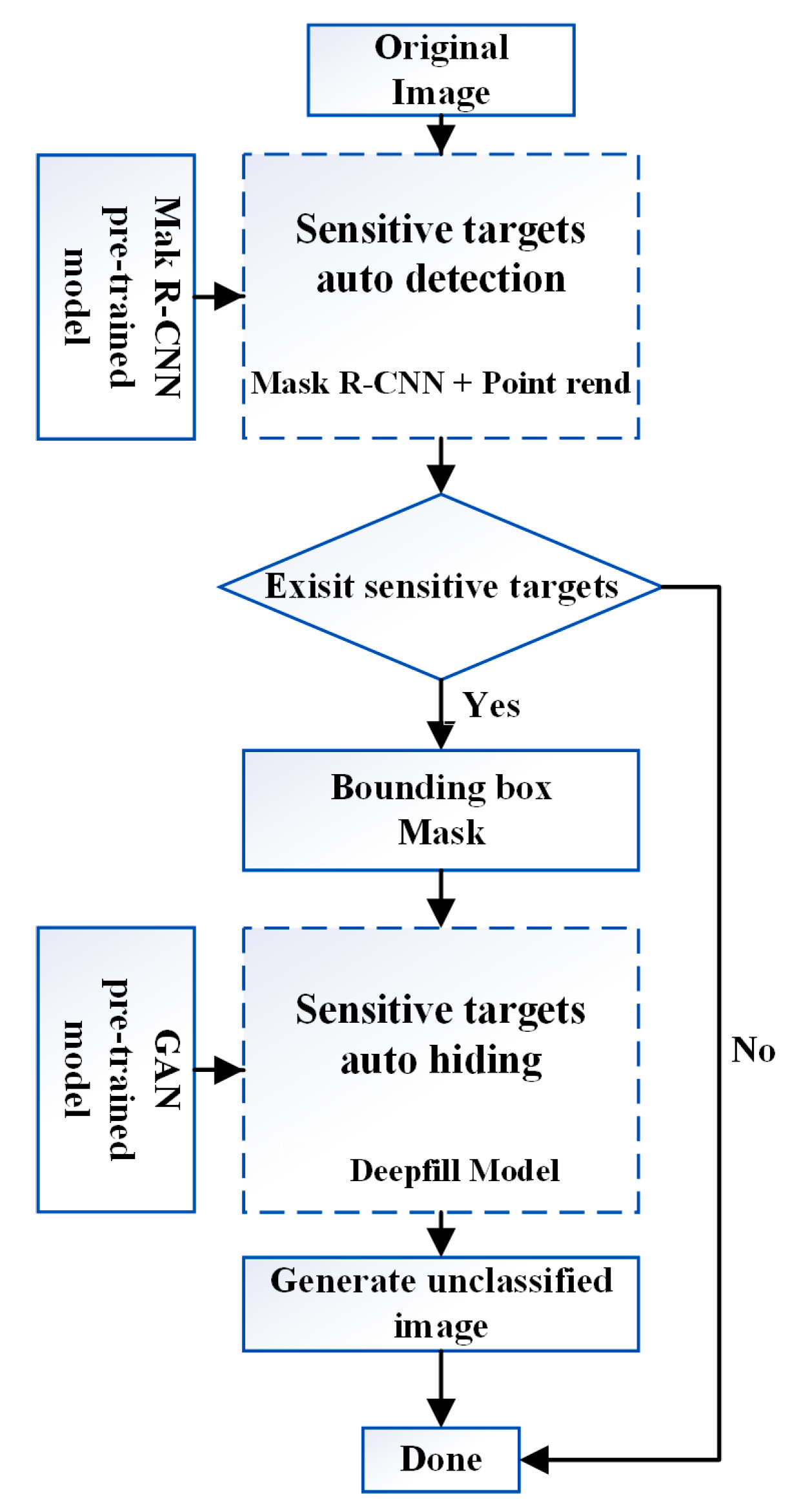
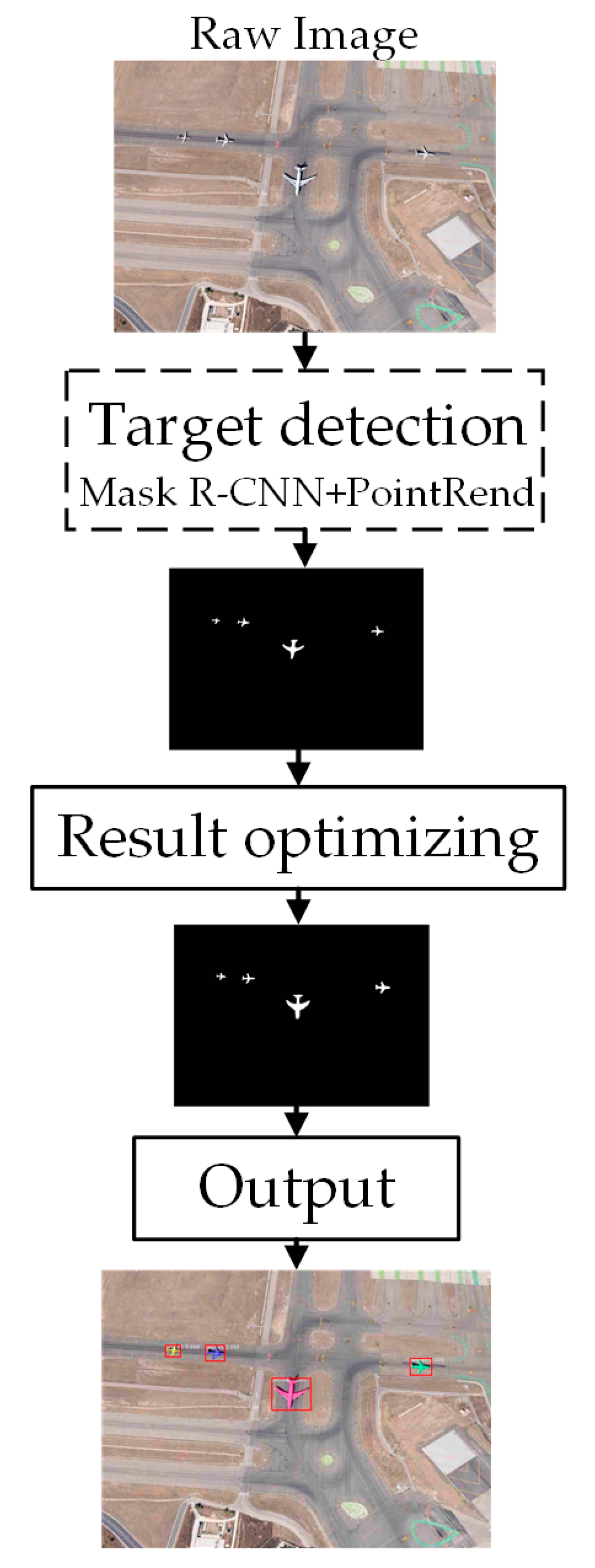
2.1. Overall Framework
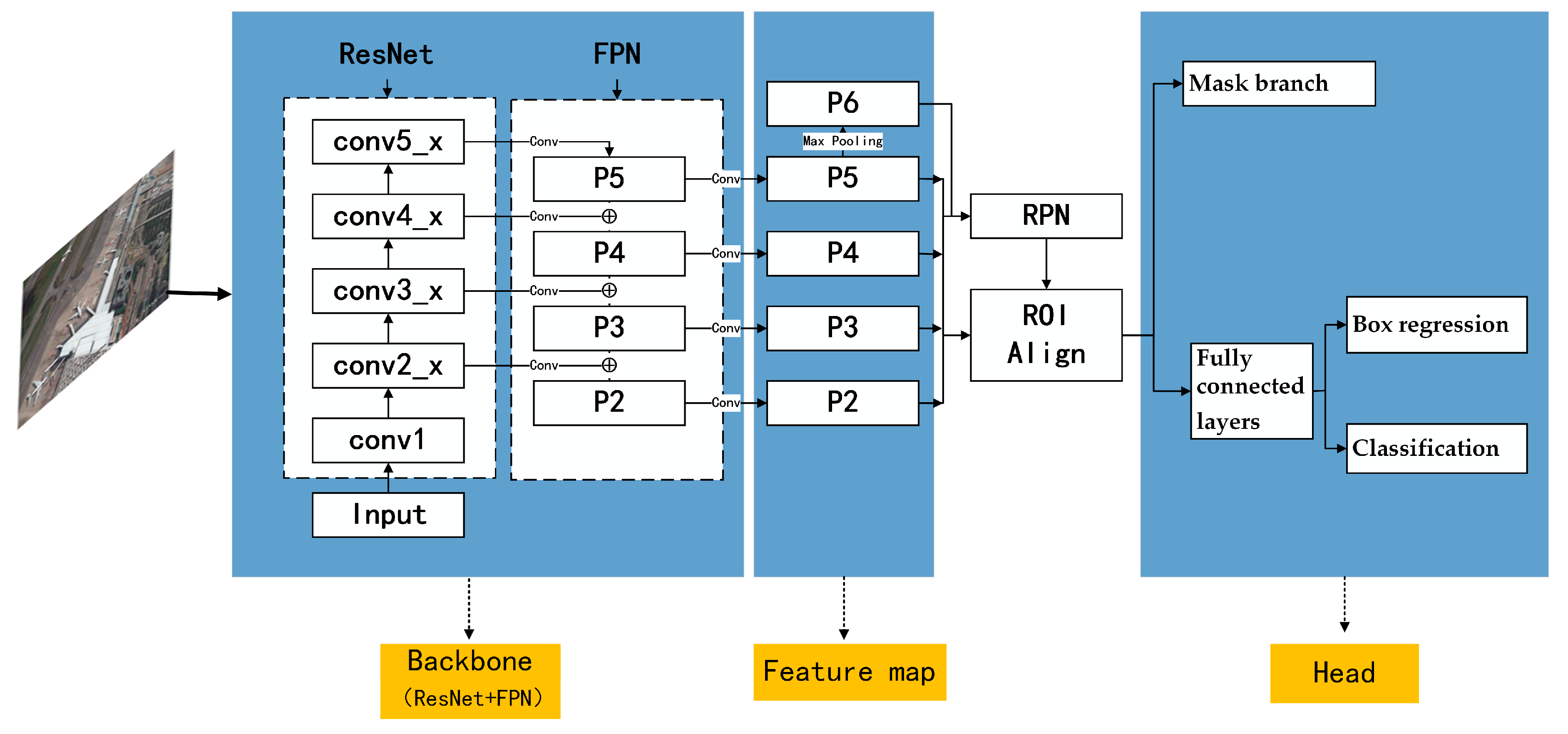
2.2. Mask R-CNN
2.2.1. Region Proposal Network (RPN)
2.2.2. RoIAlign
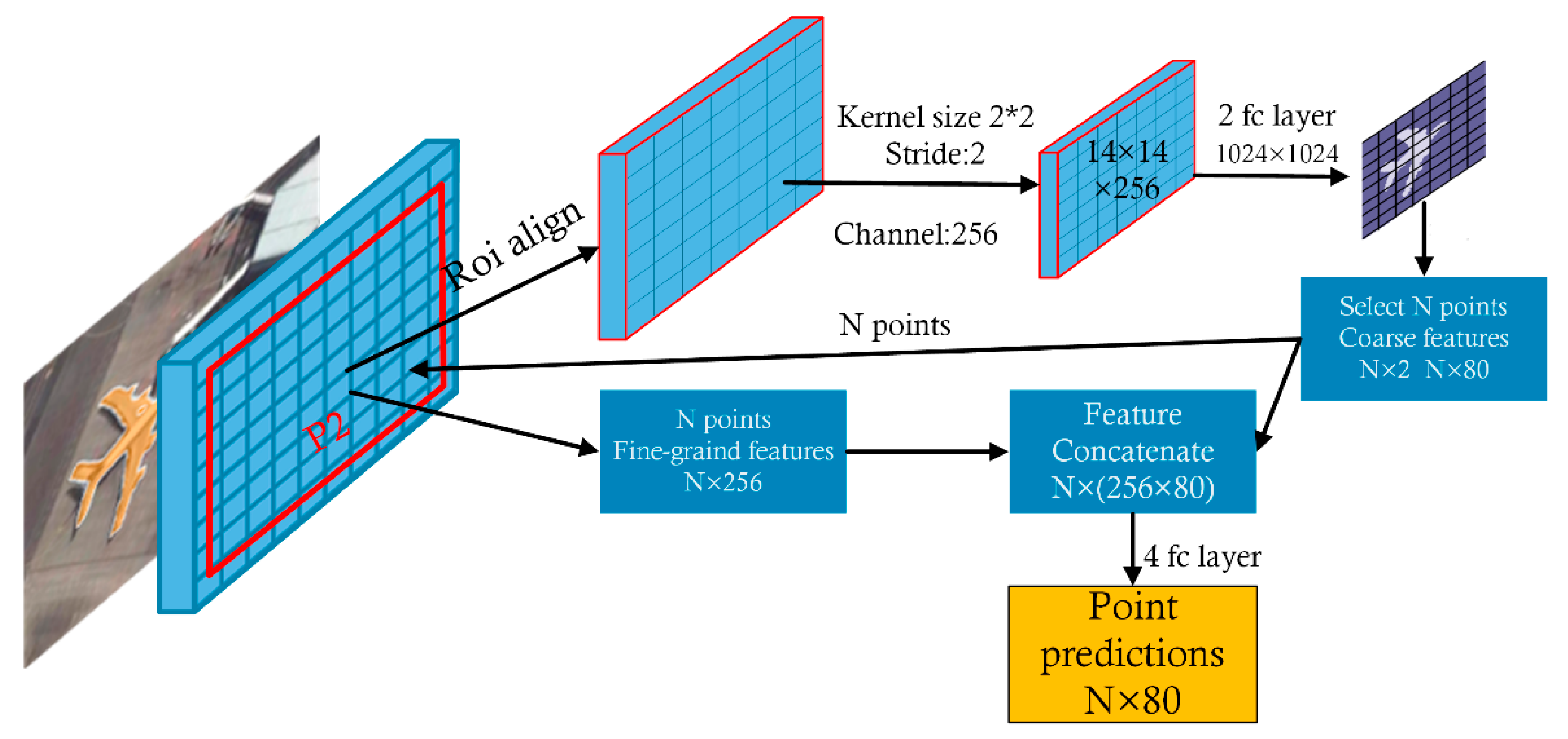
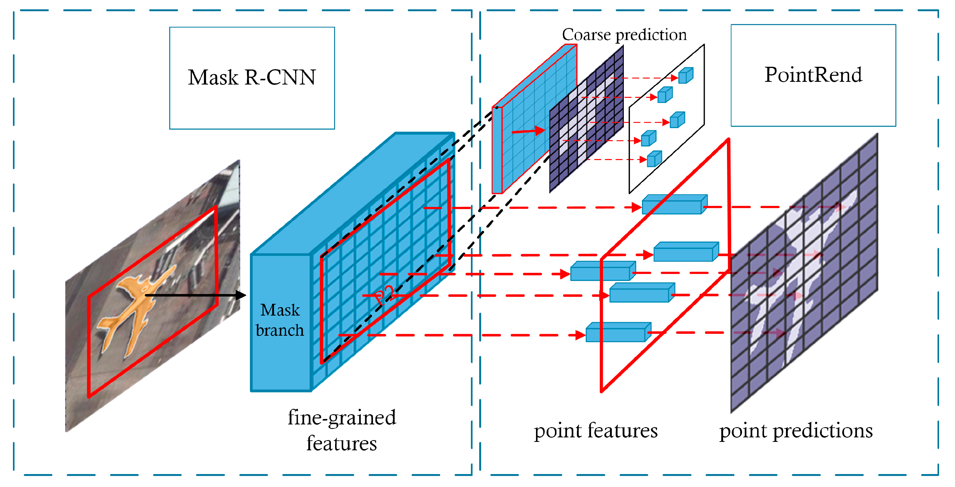
2.2.3. PointRend
- Generate a mask prediction (coarse prediction) from a lightweight coarse mask prediction head.
- Select the N “points” that are most likely to be different from their surrounding points (such as points at the edge of an object).
- For each selected point, extract a “feature representation”. This feature representation consists of two parts, i.e., fine-grained features, which are obtained through bilinear interpolation on the low-level feature map (similar to RoIAlign), and high-level features (coarse prediction), which are obtained in Step 1.
- Use a simple multilayer perceptron (MLP) to calculate a new prediction from the feature representations and update coarse prediction_i to obtain coarse prediction_i+1.
- Repeat Steps 2, 3, and 4 until the pixel requirements are met.
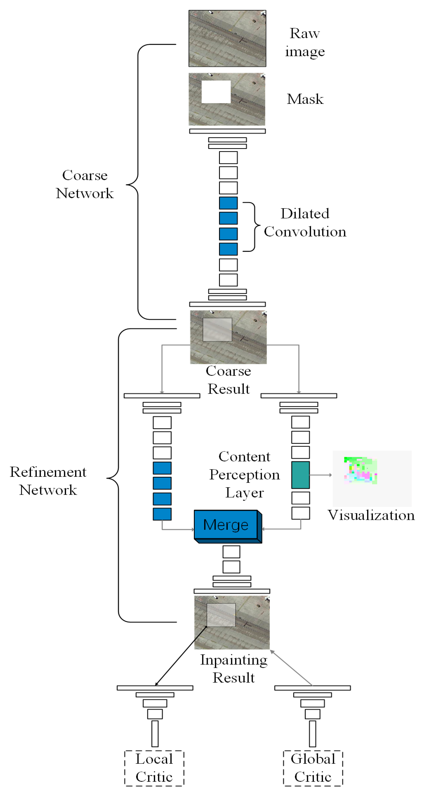
2.2.4. Deepfill
- Coarse-refinement two-stage network
- 2.
- Spatial attenuation of the reconstruction loss
2.3. Evaluation Indexes
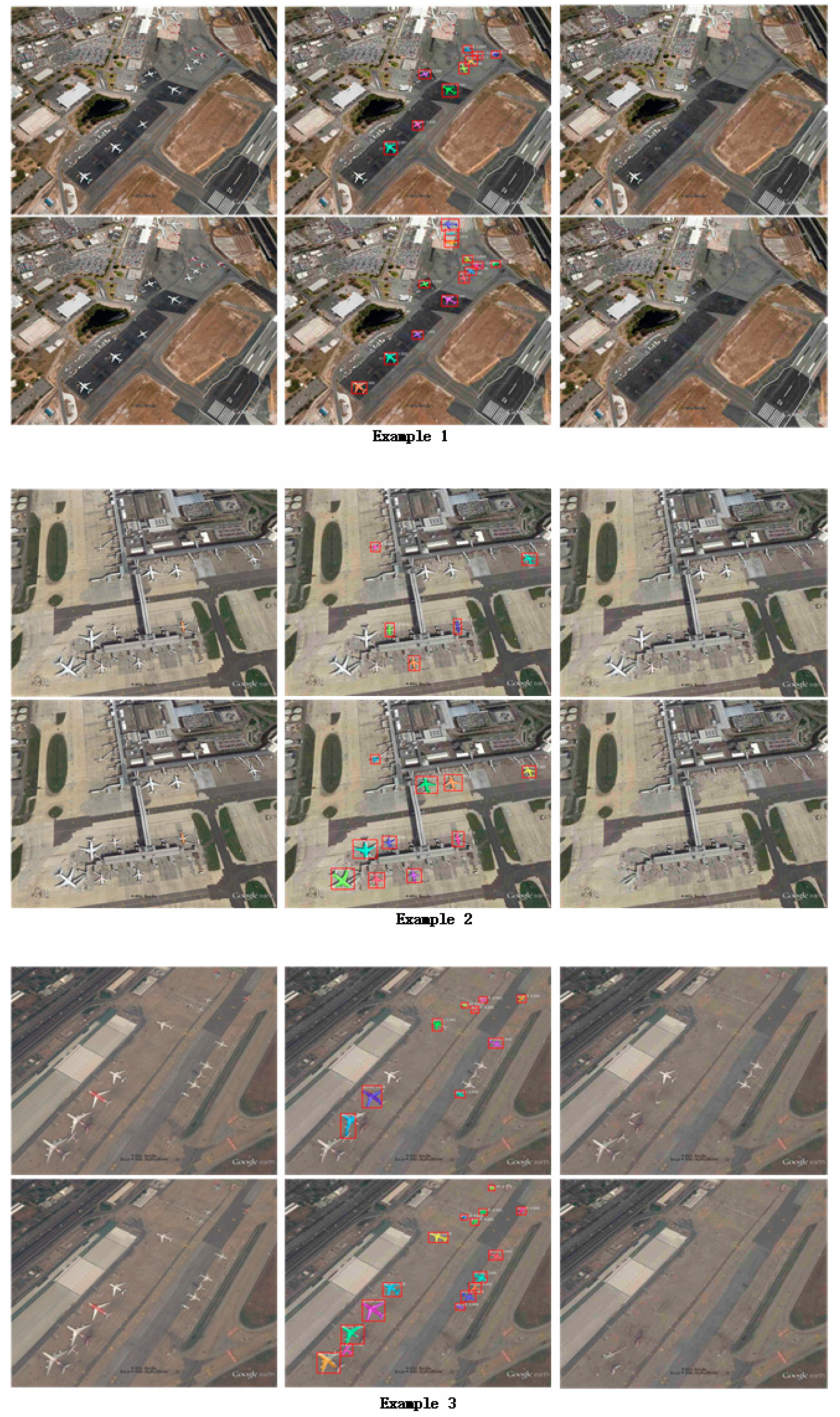
3. Application of the Two-Stage Processing Model with Aircraft Targets as an Example
3.1. Aircraft Target Characteristics
3.2. Reconstruction Loss Function of the Detection Model
3.2.1. Reconstruction Loss Function
3.2.2. Region Proposal Network (RPN) Optimization
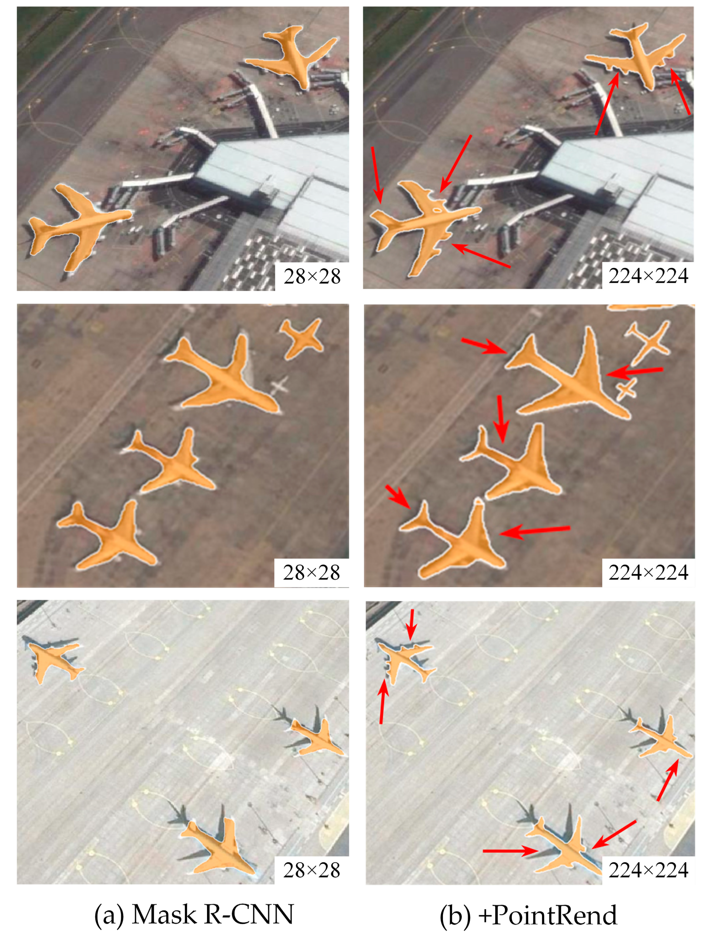
3.3. Mask R-CNN + PointRend
3.3.1. Model Structure
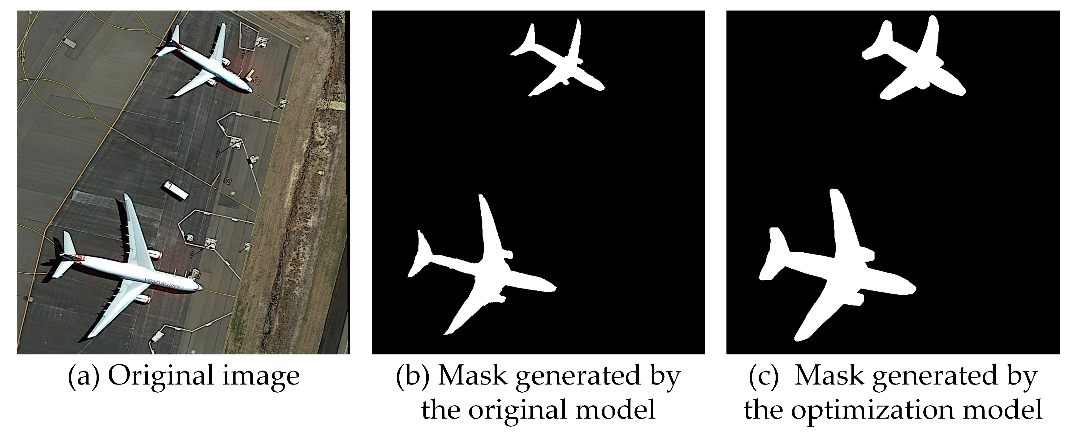
3.3.2. Mask Optimization
3.3.3. Modification of the Hiding Model Attention Mechanism
4. Experiments and Analysis
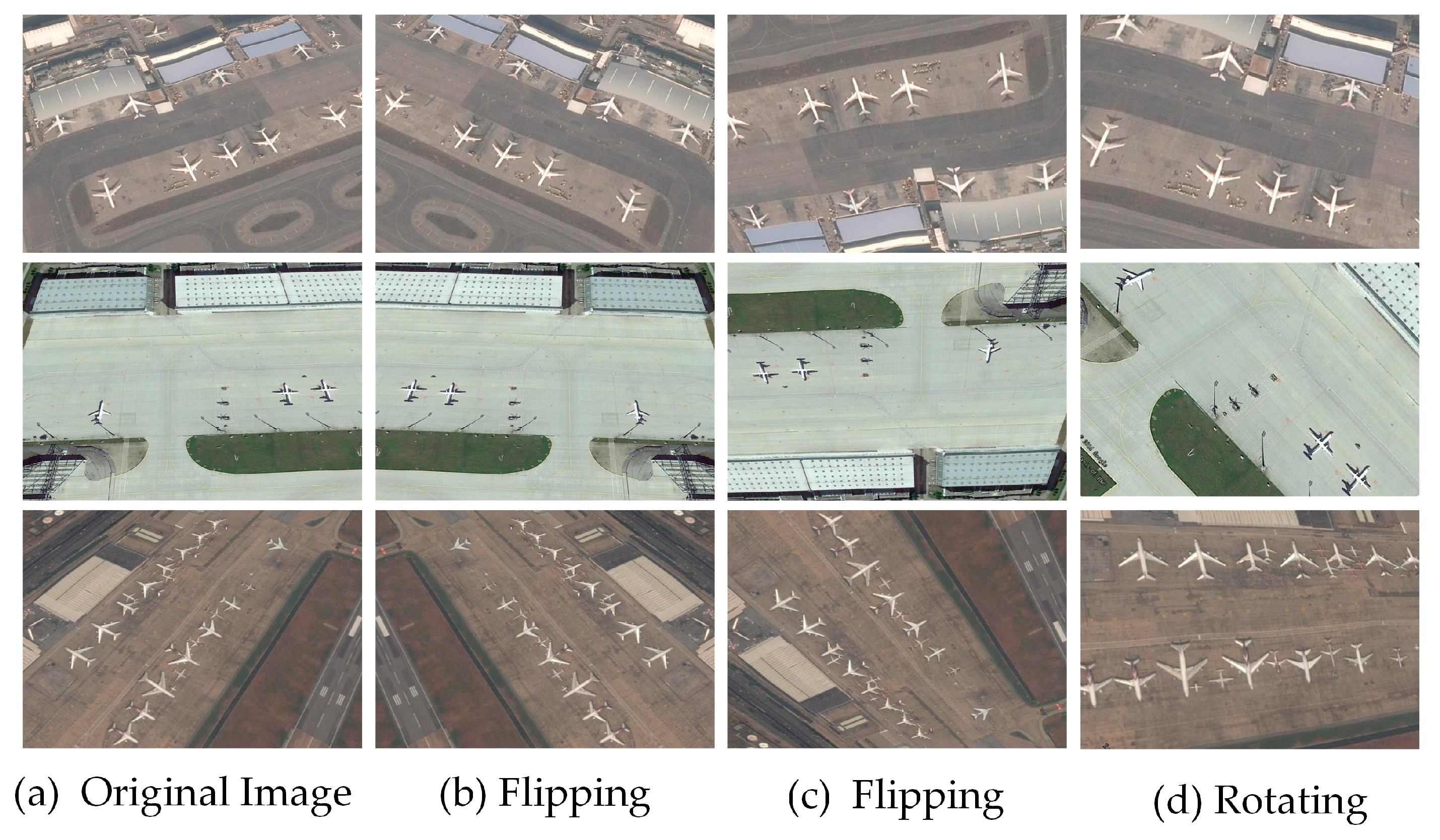
4.1. Data Collection and Preprocessing
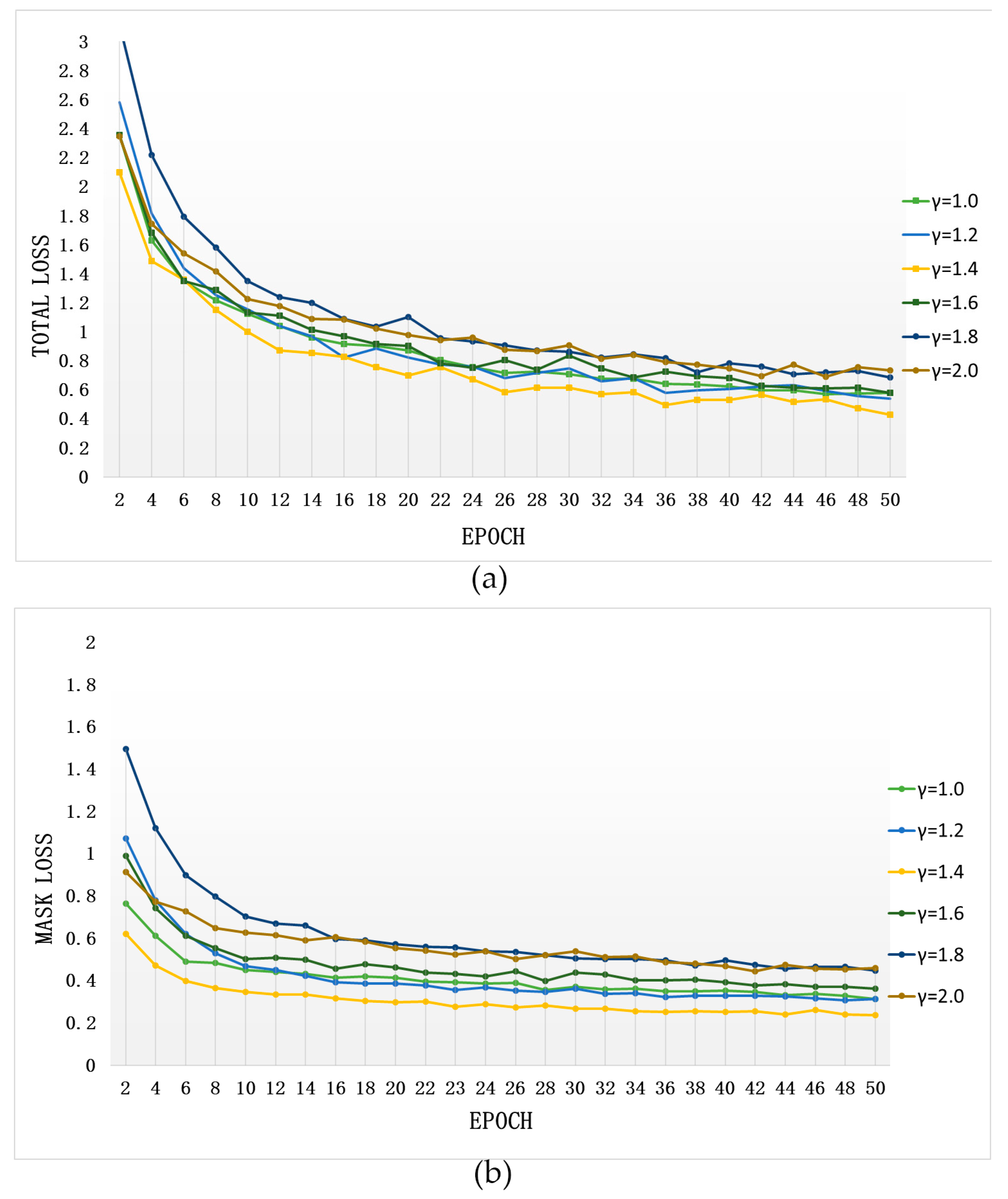
4.2. Training
4.3. Analysis of Results
4.3.1. Model Performance Analysis
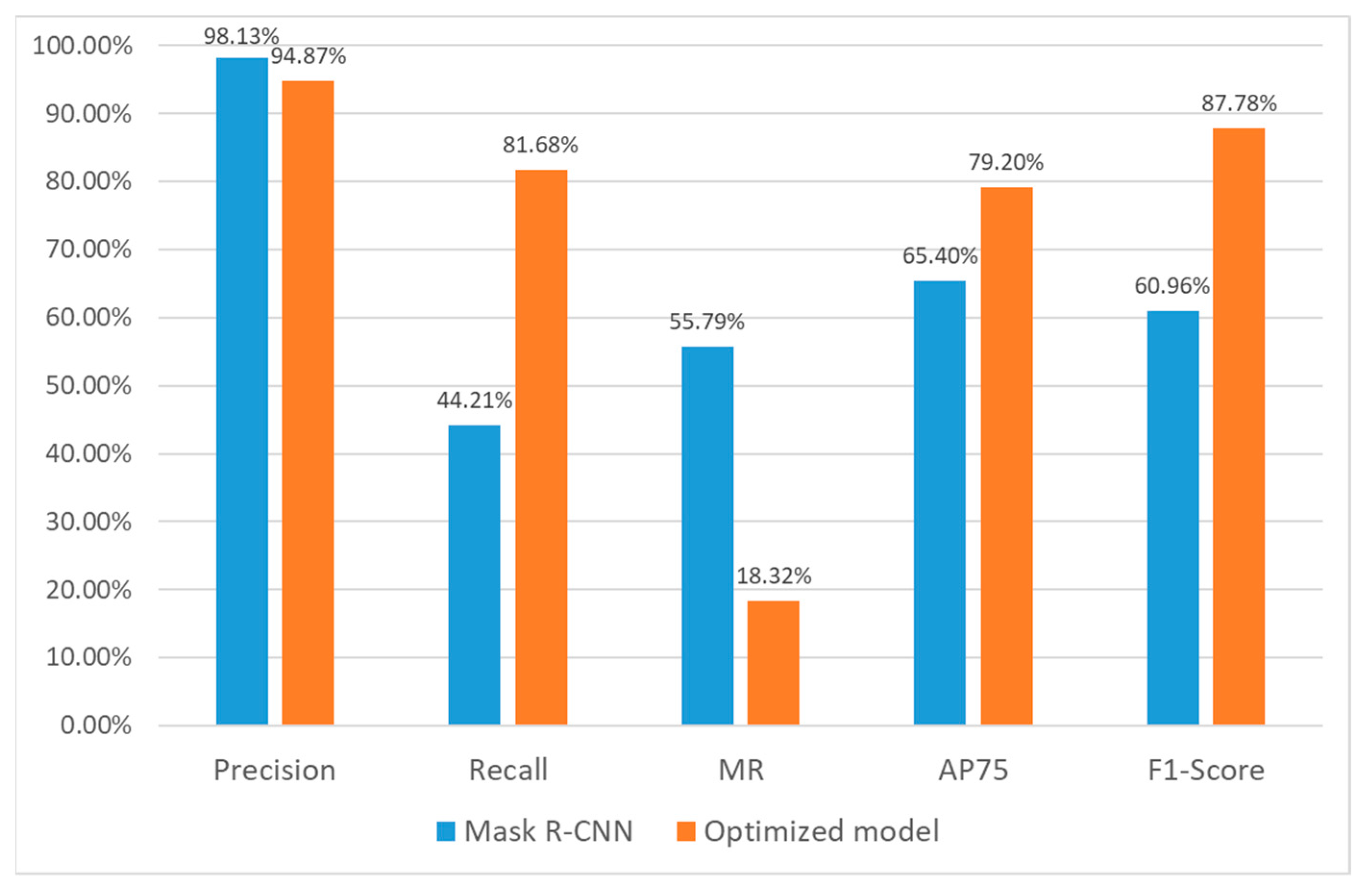
4.3.2. Comparative Analysis of Results
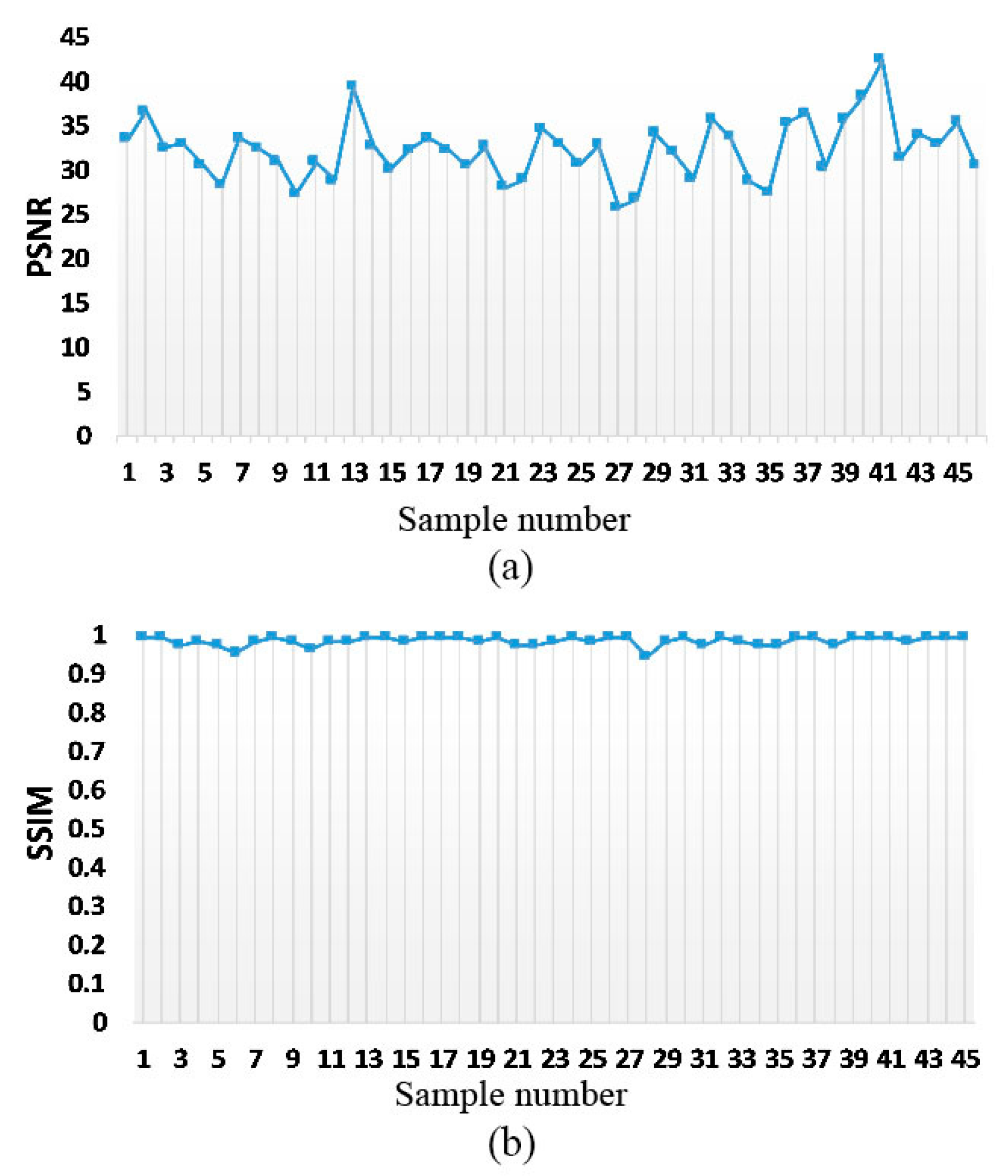
4.4. Discussion of Experimental Results
5. Conclusions
Author Contributions
Funding
Data Availability Statement
Acknowledgments
Conflicts of Interest
References
- Zhu, Q.; Cao, Z.; Lin, H.; Xie, W.; Ding, Y.L. Key technologies of emergency surveying and mapping service system. Geomat. Inf. Sci. Wuhan Univ. 2014, 39, 551–555. [Google Scholar]
- Yang, K.; Li, Q.; Fang, S. Based on remote sensing drawing monitoring, evaluate and father flood. Map 1998, 4, 22–23. (In Chinese) [Google Scholar]
- Fan, Y.D.; Yang, S.Q.; Wang, L.; Wang, W.; Nie, J.; Zhang, B.J. Study on urgent monitoring and assessment in Wenchuan earthquake. J. Remote Sens. 2008, 12, 858–864. [Google Scholar]
- Xu, T.; Zhang, J. Implementation of remote sensing automatic mapping used for earthquake emergency. J. Nat. Disasters 2017, 26, 19–27. [Google Scholar]
- Hacıefendioğlu, K.; Başağa, H.B.; Demir, G. Automatic detection of earthquake-induced ground failure effects through faster R-CNN deep learning-based object detection using satellite images. Nat. Hazards 2021, 105, 383–403. [Google Scholar] [CrossRef]
- Ghorbanzadeh, O.; Meena, S.R.; Abadi, H.S.S.; Piralilou, S.T.; Zhiyong, L.; Blaschke, T. Landslide mapping using two main deep-learning Convolution Neural Network (CNN) streams combined by the dempster—Shafer (DS) model. IEEE J. Sel. Top. Appl. Earth Obs. Remote Sens. 2020, 14. [Google Scholar] [CrossRef]
- Chen, B. Law of Surveying and Mapping of the People’s Republic of China. Available online: http://www.asianlii.org/cn/legis/cen/laws/samlotproc506/ (accessed on 5 February 2021).
- Order of the State Council of the People’s Republic of China. Available online: http://www.gov.cn/zwgk/2014-02/03/content_2579949.htm (accessed on 9 February 2021).
- Dalal, N. Histograms of oriented gradients for human detection. In Proceedings of the 2005 IEEE Computer Society Conference on Computer Vision and Pattern Recognition (CVPR’05), San Diego, CA, USA, 20–25 June 2005. [Google Scholar]
- Lowe, D.G. Distinctive image features from scale-invariant key points. Int. J. Comput. Vis. 2004, 60, 91–110. [Google Scholar] [CrossRef]
- Ojala, T.; Pietikinen, M.; Menp, T. Gray scale and rotation invariant texture classification with local binary patterns. IEEE Trans. Pattern Anal. Mach. Intell. 2000, 24, 971–987. [Google Scholar] [CrossRef]
- Bay, H.; Ess, A.; Tuytelaars, T.; Gool, L.V. Speeded-Up Robust Features (SURF). Comput. Vision Image Underst. 2008, 110, 346–359. [Google Scholar] [CrossRef]
- Wojek, C.; Schiele, B. A performance evaluation of single and multi-feature people detection. In Joint Pattern Recognition Symposium; Springer: Berlin/Heidelberg, Germany, 2008; pp. 82–91. [Google Scholar]
- Dollár, P.; Tu, Z.; Perona, P.; Belongie, S. Integral channel features. In Proceedings of the British Machine Vision Conference, London, UK, 7–10 September 2009; BMVC: London, UK, 2009. [Google Scholar]
- Zhang, Z.; Tao, W.; Sun, K.; Hu, W.; Yao, L. Pedestrian detection aided by fusion of binocular information. Pattern Recognit. 2016, 60, 227–238. [Google Scholar] [CrossRef]
- Girshick, R. Fast R-CNN. In Proceedings of the 2015 IEEE International Conference on Computer Vision (ICCV), Santiago, Chile, 7–13 December 2015; pp. 1440–1448. [Google Scholar]
- Ren, S.; He, K.; Girshick, R.; Sun, J. Faster R-CNN: Towards real-time object detection with region proposal networks. IEEE Trans. Pattern Anal. Mach. Intell. 2017, 39, 1137–1149. [Google Scholar] [CrossRef] [Green Version]
- He, K.; Georgia, G.; Piotr, D.; Ross, G. Mask R-CNN. In Proceedings of the Proceedings of the IEEE International Conference on Computer Vision (ICCV), Venice, Italy, 22–29 October 2017; pp. 2961–2969. [Google Scholar]
- Redmon, J.; Divvala, S.; Girshick, R.; Farhadi, A. You only look once: Unified, real-time object detection. In Proceedings of the 2016 IEEE Conference on Computer Vision and Pattern Recognition (CVPR), Las Vegas, NV, USA, 27–30 June 2016; pp. 779–788. [Google Scholar]
- Liu, W.; Anguelov, D.; Erhan, D.; Szegedy, C.; Reed, S.; Fu, C.; Berg, A.C. SSD: Single shot multi box detector. In Proceedings of the 14th European Conference, Amsterdam, The Netherlands, 11–14 October 2016; pp. 21–37. [Google Scholar]
- Lima, P.D.; Sensing, M.J.R. Convolutional neural network for remote-sensing scene classification: Transfer learning analysis. Remote Sens. 2020, 12, 86. [Google Scholar] [CrossRef] [Green Version]
- Fan, H.; Gui-Song, X.; Jingwen, H.; Liangpei, Z.J.R.S. Transferring deep convolutional neural networks for the scene classification of high-resolution remote sensing imagery. Remote Sens. 2015, 7, 14680–14707. [Google Scholar]
- Li, A.; Lu, Z.; Wang, L.; Xiang, T.; Wen, J.R. Zero-shot scene classification for high spatial resolution remote sensing images. IEEE Trans. Geosci. Remote Sens. 2017, 55, 4157–4167. [Google Scholar] [CrossRef]
- Chen, H.; Luo, Y.; Cao, L.; Zhang, B.; Ji, R. Generalized zero-shot vehicle detection in remote sensing imagery via coarse-to-fine framework. In Proceedings of the Twenty-Eighth International Joint Conference on Artificial Intelligence (IJCAI-19), Macao, China, 10–16 August 2019; pp. 687–693. [Google Scholar]
- Hoeser, T.; Kuenzer, C.J.R.S. Object detection and image segmentation with deep learning on earth observation data: A review—Part I: Evolution and recent trends. Remote Sens. 2020, 12, 1667. [Google Scholar] [CrossRef]
- Hoeser, T.; Bachofer, F.; Kuenzer, C.J.R.S. Object detection and image segmentation with deep learning on earth observation data: A review—Part II: Applications. Remote Sens. 2020, 12, 3053. [Google Scholar] [CrossRef]
- Lu, C. Research on Remote Sensing Image Inpainting Technology; PLA Information Engineering University: Zhengzhou, China, 2011. [Google Scholar]
- Yin, Y.; Li, D.; Hu, L. Adaptive image inpainting algorithm based on CDD model. J. Chongqing Univ. 2013, 36, 80–86. [Google Scholar]
- Barnes, C.; Shechtman, E.; Finkelstein, A.; Dan, B.G. PatchMatch: A randomized correspondence algorithm for structural image editing. ACM Trans. Graph. 2009, 28, 24. [Google Scholar] [CrossRef]
- Kirillov, A.; Wu, Y.; He, K.; Girshick, R. PointRend: Image segmentation as rendering. In Proceedings of the 2020 IEEE/CVF Conference on Computer Vision and Pattern Recognition (CVPR), Seattle, WA, USA, 13–19 June 2020; pp. 9799–9808. [Google Scholar]
- Yu, J.; Lin, Z.; Yang, J.; Shen, X.; Lu, X.; Huang, T.S. Generative image inpainting with contextual attention. In Proceedings of the 2018 IEEE/CVF Conference on Computer Vision and Pattern Recognition, Salt Lake City, UT, USA, 18–23 June 2018; pp. 5505–5514. [Google Scholar]
- He, K.; Zhang, X.; Ren, S.; Sun, J. Deep residual learning for image recognition. In Proceedings of the IEEE Conference on Computer Vision and Pattern Recognition (CVPR), Las Vegas, NV, USA, 27–30 June 2016; pp. 770–778. [Google Scholar]
- Lin, T.Y.; Dollár, P.; Girshick, R.; He, K.; Hariharan, B.; Belongie, S. Feature pyramid networks for object detection. In Proceedings of the IEEE Conference on Computer Vision and Pattern Recognition (CVPR), Honolulu, HI, USA, 21–26 July 2017; pp. 2117–2125. [Google Scholar]
- Shelhamer, E.; Long, J.; Darrell, T. Fully convolutional networks for semantic segmentation. IEEE Trans. Pattern Anal. Mach. Intell. 2017, 39, 640–651. [Google Scholar] [CrossRef] [PubMed]
- Li, X.; Liu, Z.; Luo, P.; Loy, C.C.; Tang, X. Not all pixels are equal: Difficulty-aware semantic segmentation via deep layer cascade. In Proceedings of the 2017 IEEE Conference on Computer Vision and Pattern Recognition (CVPR), Honolulu, HI, USA, 21–26 July 2017; pp. 3193–3202. [Google Scholar]
- Whitted, T. An improved illumination model for shaded display. In SIGGRAPH ‘05: ACM SIGGRAPH 2005 Courses; Association for Computing Machinery: New York, NY, USA, 1979; Volume 13, p. 14. [Google Scholar]
- Mitchell, D.P. Generating anti-aliased images at low sampling densities. In Proceedings of the 14st Annual Conference on Computer Graphics and Interactive Techniques, SIGGRAPH, August 1987; Association for Computing Machinery: New York, NY, USA, 1987. [Google Scholar]
- Zhou, K.; Hou, Q.; Wang, R.; Guo, B. Real-time KD-tree construction on graphics hardware. ACM Trans. Graph. 2008, 27, 1–11. [Google Scholar]
- Iizuka, S.; Simoserra, E.; Ishikawa, H. Globally and locally consistent image completion. ACM Trans. Graph. 2017, 36, 107. [Google Scholar] [CrossRef]
- Gulrajani, I.; Ahmed, F.; Arjovsky, M.; Dumoulin, V.; Courville, A. Improved training of Wasserstein GANs. arXiv 2017, arXiv:1704.00028. [Google Scholar]
- Woo, S.; Park, J.; Lee, J.Y.; Kweon, I.S. CBAM: Convolutional Block Attention Module. Eur. Conf. Comput. Vis. 2018, 3–19. [Google Scholar]
- Everingham, M.; Van Gool, L.; Williams, C.K.; Winn, J.; Zisserman, A. The Pascal Visual Object Classes (VOC) Challenge. Int. J. Comput. Vis. 2010, 88, 303–338. [Google Scholar] [CrossRef] [Green Version]
- Zhu, X.X.; Tuia, D.; Mou, L.; Xia, G.; Zhang, L.; Xu, F.; Fraundorfer, F. Deep learning in remote sensing: A review. IEEE Geosci. Remote Sens. Mag. 2017, 5, 8–36. [Google Scholar] [CrossRef] [Green Version]
- Han, X. Study on Key Technology of Typical Targets Recognition from Large-field Optical Remote Sensing Images. Ph.D. Dissertation, Harbin Institute of Technology, Harbin, China, 2013. [Google Scholar]
- Boeing. Available online: http://www.boeing.cn/ (accessed on 5 February 2021).
- Airbus. Available online: https://www.airbus.com/ (accessed on 5 February 2021).
- Zhe, W.; Jiexian, Z.; Qiqi, G. Aircraft target recognition in remote sensing images based on saliency images and multi-feature combination. J. Image Graph. 2017, 22, 532–541. [Google Scholar]
- Xia, G.S.; Bai, X.; Ding, J.; Zhu, Z.; Belongie, S.; Luo, J.; Datcu, M.; Pelillo, M.; Zhang, L. DOTA: A large-scale dataset for object detection in aerial images. In Proceedings of the 2018 IEEE/CVF Conference on Computer Vision and Pattern Recognition, Salt Lake City, UT, USA, 18–23 June 2018; pp. 3974–3983. [Google Scholar]
- Lin, T.Y.; Goyal, P.; Girshick, R.; He, K.; Dollár, P. Focal loss for dense object detection. IEEE Trans. Pattern Anal. Mach. Intell. 2018, 42, 318–327. [Google Scholar] [CrossRef] [PubMed] [Green Version]
- Redmon, J.; Farhadi, A. YOLOv3: An incremental improvement. arXiv 2018, arXiv:1804.02767. [Google Scholar]


| Aircraft Type | Aircraft Length (m) | Wing Length (m) | Aspect Ratio |
|---|---|---|---|
| BOEING 737-300 | 33.40 | 28.90 | 1.16 |
| BOEING 737-700 | 33.60 | 34.30 | 0.98 |
| BOEING 737-800 | 39.50 | 34.30 | 1.15 |
| BOEING 747-300 | 70.60 | 59.60 | 1.18 |
| BOEING 747-400 | 70.60 | 64.40 | 1.10 |
| BOEING 747-800 | 76.40 | 68.50 | 1.12 |
| BOEING 767-200 | 48.51 | 47.57 | 1.02 |
| BOEING 777-200 | 63.73 | 60.93 | 1.05 |
| BOEING 787-8 | 56.69 | 60.17 | 0.94 |
| BOEING 787-9 | 63.00 | 60.17 | 1.05 |
| BOEING 787-10 | 68.00 | 60.17 | 1.13 |
| AIRBUS A300 | 54.10 | 44.84 | 1.21 |
| AIRBUS A318-100 | 31.45 | 34.10 | 0.92 |
| AIRBUS A319-100 | 33.84 | 34.10 | 0.99 |
| AIRBUS A320-100 | 37.57 | 34.10 | 1.10 |
| AIRBUS A330-200 | 59.00 | 60.30 | 0.98 |
| AIRBUS A330-300 | 63.60 | 60.30 | 1.05 |
| AIRBUS A340-200 | 59.40 | 60.30 | 0.99 |
| AIRBUS A340-300 | 63.60 | 60.30 | 1.05 |
| AIRBUS A340-500 | 67.90 | 63.50 | 1.07 |
| AIRBUS A340-600 | 75.30 | 63.50 | 1.19 |
| AIRBUS A350-800 | 60.50 | 64.00 | 0.95 |
| AIRBUS A350-900 | 66.80 | 64.00 | 1.04 |
| AIRBUS A350 | 73.80 | 64.00 | 1.15 |
| AIRBUS A380-800 | 73.00 | 79.80 | 0.91 |
| Indicators | Mask R-CNN | Optimized Model |
|---|---|---|
| Number of test images | 46 | 46 |
| True target number | 475 | 475 |
| Number of detected targets | 214 | 411 |
| Number of correct detected targets | 210 | 389 |
| Number of missed targets | 265 | 86 |
| Bounding box AP75 | 65.4% | 79.2% |
Publisher’s Note: MDPI stays neutral with regard to jurisdictional claims in published maps and institutional affiliations. |
© 2021 by the authors. Licensee MDPI, Basel, Switzerland. This article is an open access article distributed under the terms and conditions of the Creative Commons Attribution (CC BY) license (http://creativecommons.org/licenses/by/4.0/).
Share and Cite
Qiu, T.; Liang, X.; Du, Q.; Ren, F.; Lu, P.; Wu, C. Techniques for the Automatic Detection and Hiding of Sensitive Targets in Emergency Mapping Based on Remote Sensing Data. ISPRS Int. J. Geo-Inf. 2021, 10, 68. https://0-doi-org.brum.beds.ac.uk/10.3390/ijgi10020068
Qiu T, Liang X, Du Q, Ren F, Lu P, Wu C. Techniques for the Automatic Detection and Hiding of Sensitive Targets in Emergency Mapping Based on Remote Sensing Data. ISPRS International Journal of Geo-Information. 2021; 10(2):68. https://0-doi-org.brum.beds.ac.uk/10.3390/ijgi10020068
Chicago/Turabian StyleQiu, Tianqi, Xiaojin Liang, Qingyun Du, Fu Ren, Pengjie Lu, and Chao Wu. 2021. "Techniques for the Automatic Detection and Hiding of Sensitive Targets in Emergency Mapping Based on Remote Sensing Data" ISPRS International Journal of Geo-Information 10, no. 2: 68. https://0-doi-org.brum.beds.ac.uk/10.3390/ijgi10020068